Data-Free Dynamic Compression of CNNs for Tractable Efficiency
Lukas Meiner
1,2 a
, Jens Mehnert
1 b
and Alexandru Paul Condurache
1,2 c
1
Cross-Domain Computing Solutions, Robert Bosch GmbH, Daimlerstraße 6, 71229 Leonberg, Germany
2
Institute for Signal Processing, Universit
¨
at zu L
¨
ubeck, Ratzeburger Allee 160, 23562 L
¨
ubeck, Germany
Keywords:
Model Compression, Structured Pruning, Hashing, Data-Free, CNNs.
Abstract:
To reduce the computational cost of convolutional neural networks (CNNs) on resource-constrained devices,
structured pruning approaches have shown promise in lowering floating-point operations (FLOPs) without
substantial drops in accuracy. However, most methods require fine-tuning or specific training procedures
to achieve a reasonable trade-off between retained accuracy and reduction in FLOPs, adding computational
overhead and requiring training data to be available. To this end, we propose HASTE (Hashing for Tractable
Efficiency), a data-free, plug-and-play convolution module that instantly reduces a network’s test-time inference
cost without training or fine-tuning. Our approach utilizes locality-sensitive hashing (LSH) to detect redundan-
cies in the channel dimension of latent feature maps, compressing similar channels to reduce input and filter
depth simultaneously, resulting in cheaper convolutions. We demonstrate our approach on the popular vision
benchmarks CIFAR-10 and ImageNet, where we achieve a 46.72% reduction in FLOPs with only a 1.25% loss
in accuracy by swapping the convolution modules in a ResNet34 on CIFAR-10 for our HASTE module.
1 INTRODUCTION
With the rise in availability and capability of deep
learning hardware, the possibility to train ever larger
models led to impressive achievements in the field of
computer vision. At the same time, concerns regarding
high computational costs, environmental impact and
the applicability on resource-constrained devices are
growing. This led to the introduction of carefully con-
structed efficient models (Howard et al., 2017; Sandler
et al., 2018; Tan and Le, 2019, 2021; Zhang et al.,
2018; Ma et al., 2018) that offer fast inference in
embedded applications, gaining speed by introduc-
ing larger inductive biases. Yet, highly scalable and
straight-forward architectures (Simonyan and Zisser-
man, 2015; He et al., 2016; Dosovitskiy et al., 2021;
Liu et al., 2021b, 2022; Woo et al., 2023) remain pop-
ular due to their performance and ability to generalize,
despite requiring more data, time and energy to train.
To still allow for larger models to be used in mobile
applications, various methods (Zhang et al., 2016; Lin
et al., 2017b; Pleiss et al., 2017; Han et al., 2020; Luo
et al., 2017) have been proposed to reduce their com-
putational cost. One particularly promising field of
a
https://orcid.org/0009-0003-1451-2197
b
https://orcid.org/0000-0002-0079-0036
c
https://orcid.org/0000-0002-0626-335X
research for the compression of convolutional archi-
tectures is pruning (Wimmer et al., 2023), especially
in the form of structured pruning for direct resource
savings (Anwar et al., 2017).
However, the application of existing work is re-
stricted by two factors. Firstly, many proposed ap-
proaches rely on actively learning which channels
to prune during the regular model training procedure
(Dong et al., 2017; Liu et al., 2017; Gao et al., 2019;
Verelst and Tuytelaars, 2020; Bejnordi et al., 2020; Li
et al., 2021; Xu et al., 2021). This introduces additional
parameters to the model, increases the complexity of
the optimization process due to supplementary loss
terms, and requires existing models to be retrained to
achieve any reduction in FLOPs. The second limit-
ing factor is the necessity of performing fine-tuning
steps to restore the performance of pruned models
back to acceptable levels (Wen et al., 2016; Li et al.,
2017; Lin et al., 2017a; Zhuang et al., 2018; He et al.,
2018). Aside from the incurred additional cost and
time requirements, this creates a dependency on the
availability of the data that was originally used to train
the baseline model, as tuning the model on a different
set of data can lead to catastrophic forgetting (Good-
fellow et al., 2014).
To this end, we propose HASTE, a plug-and-play
channel pruning approach that is entirely data-free and
196
Meiner, L., Mehnert, J. and Condurache, A. P.
Data-Free Dynamic Compression of CNNs for Tractable Efficiency.
DOI: 10.5220/0013301000003912
Paper published under CC license (CC BY-NC-ND 4.0)
In Proceedings of the 20th International Joint Conference on Computer Vision, Imaging and Computer Graphics Theory and Applications (VISIGRAPP 2025) - Volume 2: VISAPP, pages
196-208
ISBN: 978-989-758-728-3; ISSN: 2184-4321
Proceedings Copyright © 2025 by SCITEPRESS – Science and Technology Publications, Lda.

Training
Fine-Tuning
HASTE
Module
Untrained
Network
Trained
Network
Pruned
Network
(a) Training-Based (b) Tuning-Based
(c) Instant Pruning (Ours)
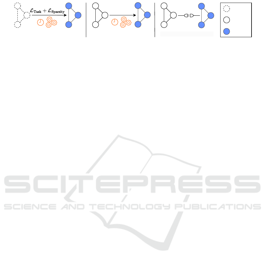
Figure 1: Overview of related pruning approaches. Training-based methods require specialized training procedures. Methods
based on fine-tuning need retraining to compensate lost accuracy in the pruning step. Our method instantly reduces network
FLOPs and maintains high accuracy entirely without training or fine-tuning.
does not require any real or synthetic training data.
Our method instantly reduces the computational com-
plexity of convolution modules without requiring any
additional training or fine-tuning. To achieve this, we
utilize a locality-sensitive hashing scheme (Indyk and
Motwani, 1998) to dynamically detect and cluster simi-
larities in the channel dimension of latent feature maps
in CNNs. By exploiting the distributive property of the
convolution operation, we take the average of all input
channels that are found to be approximately similar
and convolve it with the sum of corresponding filter
channels. This reduced convolution is performed on a
smaller channel dimension, which drastically lowers
the amount of FLOPs required. The trade-off between
retained accuracy and compression ratio is directly
steerable by altering one hyperparameter shared across
all HASTE modules in the network, which simplifies
experimentation for users.
Our experiments demonstrate that the HASTE
module is capable of greatly reducing computational
cost of a wide variety of pre-trained CNNs while main-
taining high accuracy. More importantly, it does so
directly after exchanging the original convolutional
modules for the HASTE block. This allows us to skip
lengthy model trainings with additional regularization
and sparsity losses as well as extensive fine-tuning
procedures. Furthermore, we are not tied to the avail-
ability of the dataset on which the given model was
originally trained. Our pruning approach is entirely
data-free, thus enabling pruning in a setup where ac-
cess to the trained model is possible, but access to the
data is restricted. Finally, this allows us to adjust the
computational cost of a model in real time, adapting
its test-time complexity to the availability of hardware
resources. To the best of our knowledge, this makes
the HASTE module the first dynamic and data-free
CNN pruning approach that does not require any form
of training or fine-tuning.
Our main contributions are:
• We propose a locality-sensitive hashing based
method to dynamically detect redundancies in the
latent features of current CNN architectures. Our
method incurs a low computational overhead and
is entirely data-free.
• We propose HASTE, a scalable, plug-and-play con-
volution module replacement that leverages these
structural redundancies to save computational com-
plexity in the form of FLOPs at test time, without
requiring any training steps.
• We showcase our method’s performance on pop-
ular CNN models trained on benchmark vision
datasets. We also identify a positive scaling behav-
ior, achieving higher cost reductions on deeper and
wider models.
2 RELATED WORK
When structurally pruning a model, its computational
complexity is reduced at the expense of performance
on a given task. For this reason, fine-tuning is often
performed after the pruning scheme was applied. The
model is trained again in its pruned state to compensate
the loss of structural components, often requiring mul-
tiple epochs of tuning (Li et al., 2017; Zhuang et al.,
2018; Xu et al., 2021) on the training dataset. These
methods tend to remove structures from models in a
static way, not adjusting for different degrees of spar-
sity across varying input data. Some recent methods
avoid fine-tuning by learning a pruning pattern during
regular model training (Liu et al., 2017; Gao et al.,
2019; Xu et al., 2021; Li et al., 2021; Elkerdawy et al.,
2022). This generates an input-dependent dynamic
path through the network, allocating less compute to
sparser images.
Static Pruning. By finding general criteria for the im-
portance of individual channels, some recent methods
propose static pruning approaches. PFEC (Li et al.,
2017) prunes filter kernels with low importance mea-
sured by their L
1
-norm in a one-shot manner. DCP
(Zhuang et al., 2018) equips models with multiple loss
terms before fine-tuning to promote highly discrimina-
tive channels to be formed. Then, a channel selection
algorithm picks the most informative ones. FPGM
(He et al., 2019) demonstrates a fine-tuning-free prun-
ing scheme, exploiting norm-based redundancies to
train models with reduced complexity. AMC (He et al.,
2018) explores a compression policy generated by rein-
Data-Free Dynamic Compression of CNNs for Tractable Efficiency
197

forcement learning. A handful of data-free approaches
exist, yet they either use synthetic data to retrain the
model (Yin et al., 2020) or generate a static model
(Yvinec et al., 2023; Bai et al., 2023) that is unable to
adapt its compression to the availability of hardware re-
sources on the fly. We target the dynamic compression
of models in a data-free manner.
Dynamic Gating. To accommodate inputs of vary-
ing complexity in the pruning process, recent works
try to learn dynamic, input-dependent paths through
the network (Xu et al., 2021; Li et al., 2021; Elker-
dawy et al., 2022; Liu et al., 2017; Hua et al., 2019;
Verelst and Tuytelaars, 2020; Bejnordi et al., 2020; Liu
et al., 2019). These methods learn (binary) masks that
toggle structural components of the underlying CNN
at runtime. This requires storing all of the model’s
weights, as each weight is potentially important for
specific inputs. DGNet (Li et al., 2021) equips the
base model with additional spatial and channel gating
modules based on average pooling that are trained end-
to-end together with the model using additional regu-
larization losses. Similarly, DMCP (Xu et al., 2021)
learns mask vectors using a pruning loss and does
not need fine-tuning procedures after training. FTWT
(Elkerdawy et al., 2022) decouples the task and regu-
larization losses introduced by previous approaches,
reducing the complexity of the pruning scheme. While
these methods do not require fine-tuning, they intro-
duce additional complexity through pruning losses and
the need for custom gating modules during training
to realize FLOP savings. We focus on real-time com-
pression during model inference, with no training and
data requirement at all. This also enables us to have
tractable compression ratios at test time, as we do not
require training towards a set ratio.
Hashing for Efficient Inference. In recent years, the
usage of locality-sensitive hashing (Indyk and Mot-
wani, 1998) schemes as a means to make model in-
ference more efficient has gained some popularity.
Reformer (Kitaev et al., 2020) uses LSH to reduce
the computational complexity of multi-head attention
modules in transformer models by finding similar
queries and keys before computing their matrix prod-
uct. M
¨
uller et al. (2022) employ a multiresolution hash
encoding to construct an efficient feature embedding
for neural radiance fields (NeRFs), leading to orders
of magnitude speedup compared to previous methods.
SLIDE (Chen et al., 2020) and MONGOOSE (Chen
et al., 2021) use a similar LSH scheme to store non-
contiguous activation patterns of a high-dimensional
feedforward network, only computing the strongest
activating neurons during the forward pass. Using spe-
cialized C++ and CUDA code, the authors achieve
significant speedups on CPUs as well as GPUs. Other
approaches related to LSH have also been explored for
model compression. Liu et al. (2021a) employ a count
sketch-type algorithm to approximate the forward pass
of multilayer perceptrons by hashing the model’s input
vector. FPKM (Liu et al., 2021c) extends on FPGM
(He et al., 2019) and explores the use of k -means clus-
tering for finding redundant input channels. However,
this approach is limited to fixed pruning ratios deter-
mined by the amount of clusters, and does not allow
for dynamic compression.
3 METHOD
In this section, we present HASTE, a novel convolu-
tion module based on locality-sensitive hashing that
acts as a plug-and-play replacement for any regular
convolution module, instantly reducing the FLOPs dur-
ing inference. Firstly, we give a formal definition of
the underlying LSH scheme. Secondly, we illustrate
how hashing is used to identify redundancies inside
latent features of convolutional network architectures.
Lastly, we present the integration of the hashing pro-
cess into our proposed HASTE module, which allows
us to compress latent features for cheaper computa-
tions.
3.1 Locality-Sensitive Hashing via
Sparse Random Projections
Locality-sensitive hashing is a popular approach for
approximate fast nearest neighbor search in high-
dimensional spaces. A hash function h : R
d
→ N is
locality-sensitive, if similar vectors in the input domain
x,y ∈ R
d
receive the same hash codes h(x) = h(y) with
high probability. This is in contrast to regular hash-
ing schemes which try to reduce hash collisions to a
minimum, widely scattering the input data across their
hash buckets. More formally, we require a measure
of similarity on the input space and an adequate hash
function h . A particularly suitable measure for use
in convolutional architectures is the cosine similarity,
as convolving the (approximately) normalized kernel
with the normalized input is equivalent to computing
their cosine similarity. Pairwise similarities between
vectors are preserved through hashing by the allocation
of similar hash codes.
One particular family of hash functions that groups
input data by cosine similarity is given by random
projections (RP). These functions partition the high-
dimensional input space through L random hyper-
planes, such that each input vector is assigned to ex-
actly one section of this partitioning, called a hash
bucket. Determining the position of an input x ∈ R
d
VISAPP 2025 - 20th International Conference on Computer Vision Theory and Applications
198

Extract Patch
Input Patch
Input Feature Map
Convolutional Filters
Redundancy-Free
Patch
Redundancy-Free
Convolutional Filters
Output Feature Map
Hash Channels to
Find Redundancies
Compute Mean
per Bucket
Convolve
Sum Corresponding
Channels on Copy of Filters
Buckets
Empty
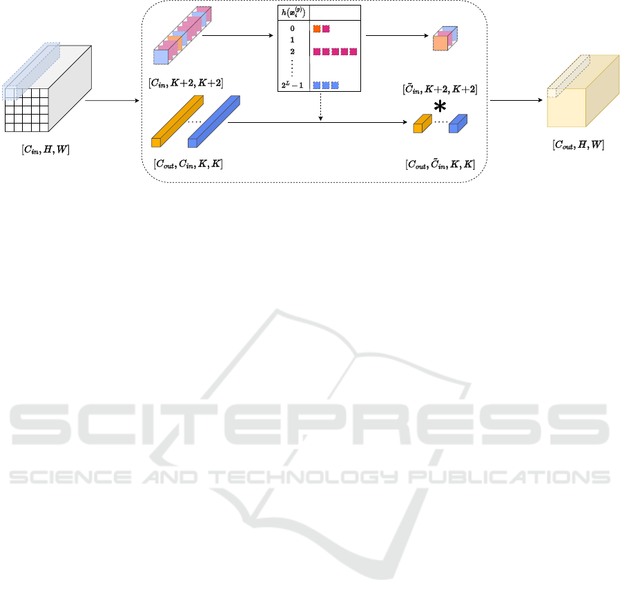
Figure 2: Overview of our proposed HASTE module. Each patch of the input feature map is processed to find redundant
channels. Detected redundancies are then merged together, dynamically reducing the depth of each patch and the convolutional
filters.
relative to all L hyperplanes is done by computing
the dot product with their normal vectors v
l
∈ R
d
, l ∈
{1,...,L}
, whose entries are drawn from a standard
normal distribution N(0,1). By defining
h
l
: R
d
→ {0, 1}, h
l
(x) :=
(
1, if v
l
· x > 0,
0, else,
(1)
we get a binary information representing to which side
of the l -th hyperplane input x lies. The hyperparame-
ter L governs the discriminative power of this method,
dividing the input space R
d
into a total of 2
L
distinct re-
gions, or hash buckets. By concatenating all individual
functions h
l
, we receive the RP hash function
h : R
d
→ {0, 1}
L
, h(x) = (h
1
(x),...,h
L
(x)). (2)
Note that h(x) is an L -bit binary code, acting as an
identifier of exactly one of the 2
L
hash buckets. Equiv-
alently, we can transform this code into an integer,
labeling the hash buckets from 0 to 2
L
− 1:
h : R
d
→

0,...,2
L
− 1

h(x) = 2
L−1
h
L
(x) + · · · + 2
0
h
1
(x).
(3)
While LSH already reduces computational com-
plexity drastically compared to exact nearest neighbor
search, the binary code generation still requires L · d
multiplications and L · (d − 1) additions per input. To
further decrease the cost of this operation, we em-
ploy the method presented by (Achlioptas, 2003; Li
et al., 2006): Instead of using standard normally dis-
tributed vectors v
l
, we use very sparse vectors ˜v
l
, con-
taining only elements from the set {1,0,−1} . Given a
targeted degree of sparsity s ∈ (0, 1) , the hyperplane
normal vectors ˜v
l
are constructed randomly such that
the expected ratio of zero entries is s . The remaining
1 − s of vector components are randomly filled with
either 1 or −1 , both chosen with equal probability.
This reduces the dot product computation to a total of
L·(d(1−s)−1) additions and 0 multiplications, as we
only need to sum entries of x where ˜v
l
is non-zero with
the corresponding signs. Consequently, this allows us
to trade expensive multiplication operations for cheap
additions.
3.2 Finding Redundancies with LSH
After establishing LSH via sparse random projections
as a computationally cheap way to find approximate
nearest neighbors in high-dimensional spaces, we now
aim to leverage this method as a means of finding
redundancies in the channel dimension of latent feature
maps in CNNs. Formally, a convolutional layer can
be described by sliding multiple learned filters F
j
∈
R
C
in
×K×K
, j ∈ {1,.. . ,C
out
} over the (padded) input
feature map X ∈ R
C
in
×H×W
and computing the discrete
convolution at every point. Here, K is the kernel size,
H and W denote the spatial dimensions of the input,
and C
in
,C
out
describe the input and output channel
dimensions, respectively.
For any filter position, the corresponding input
window contains redundant information in the form
of similar channels. However, a regular convolution
module ignores potential savings from reducing the
amount of similar computations in the convolution
process. We challenge this design choice and instead
leverage redundant channels to save computations in
the convolution operation. As the first step, we ras-
terize the (padded) input feature map into patches
X
(p)
i
∈ R
(K+2)×(K+2)
for i = 1,... ,C
in
, with an overlap
of two pixels on each side. This is equivalent to split-
ting the spatial dimension into patches of size K × K ,
but keeping the filter overlap to its neighbors. The
special case of K = 1 is discussed in Appendix .1.
To group similar channels together, we flatten all
individual channels X
(p)
i
into vectors of dimension
(K + 2)
2
and center them by the mean along the chan-
nel dimension for any given patch p . We denote the
Data-Free Dynamic Compression of CNNs for Tractable Efficiency
199

resulting vectors as x
(p)
i
. Finally, they are hashed us-
ing h , giving us a total of C
in
hash codes. We then
check which hash code appears more than once, as all
elements that appear in the same hash bucket are deter-
mined to be approximately similar by the LSH scheme.
Consequently, grouping the vector representations of
X
(p)
i
by their hash code, we receive sets of redundant
feature map channels.
In particular, note that our RP LSH approach is
invariant to the scaling of a given input vector. This
means that input channels of the same spatial structure,
but with different activation intensities, still land in
the same hash bucket, effectively finding even more
redundancies in the channel dimension.
3.3 The HASTE Module
Our approach is motivated by the distributivity of the
convolution operation. Instead of convolving various
filter kernels with nearly similar input channels and
summing the result, we can approximate this operation
by computing the sum of kernels first and convolving
it with the mean of these redundant channels. The
grouping of input channels X
(p)
i
into hash buckets pro-
vides a straight-forward way to utilize this distributive
property for the reduction of required floating-point
operations when performing convolutions.
To avoid repeated computations on nearly similar
channels, we dynamically reduce the size of each input
context window X
(p)
by compressing channels found
in the same hash bucket, as shown in Figure 2. The
merging operation is performed by taking the mean of
all channels in one bucket. As a result, the number of
remaining input channels of a given patch is reduced
to
˜
C
in
< C
in
. In a similar manner to the reduction of
the input feature map depth, we add the corresponding
channels of all convolutional filters F
j
. Note that this
does not require hashing of the filter channels, as we
can simply aggregate those kernels that correspond
to the collapsed input channels. This step is done on
the fly for every patch p , retaining the original filter
weights for the next patch.
The choice of different merging operations for in-
put and filter channels is directly attributable to the
distributive property, as the convolution between the
average input and summed filter set retains a similar
output intensity to the original convolution. When
choosing to either average or sum both inputs and fil-
ters, we would systematically under- or overestimate
the original output, respectively.
Finally, the reduced input patch is convolved with
the reduced set of filters in a sliding window manner to
Table 1: Overview of related pruning approaches. While
other methods require either fine-tuning or a specialized
training procedure to achieve notable FLOPs reduction, our
method is completely training-free and data-free.
Method Dynamic
Restrictive Requirements
Training Fine-Tuning Data Availability
SSL (Wen et al., 2016) ✗ ✗ ✓ ✓
PFEC (Li et al., 2017) ✗ ✗ ✓ ✓
LCCN (Dong et al., 2017) ✓ ✓ ✗ ✓
FBS (Gao et al., 2019) ✓ ✓ ✗ ✓
FPGM (He et al., 2019) ✗ ✓ ✗ ✓
DynConv (Verelst and Tuytelaars, 2020) ✓ ✓ ✗ ✓
DMCP (Xu et al., 2021) ✓ ✓ ✗ ✓
DGNet (Li et al., 2021) ✓ ✓ ✗ ✓
FTWT (Elkerdawy et al., 2022) ✓ ✓ ✗ ✓
HASTE (ours) ✓ ✗ ✗ ✗
compute the output. This can be formalized as follows:
C
in
∑
i=1
F
j,i
∗ X
(p)
i
≈
2
L
−1
∑
l=0
S
(p)
l
̸=
/
0

∑
i∈S
(p)
l
F
j,i

∗

1
|S
(p)
l
|
∑
i∈S
(p)
l
X
(p)
i

!
,
(4)
where S
(p)
l
= {i ∈ {1,... ,C
in
}|h(x
(p)
i
) = l} contains
all channel indices that appear in the l-th hash bucket.
Since we do not remove entire filters, but rather reduce
their depth, the output feature map retains the same
spatial dimension and number of channels as with a
regular convolution module. The entire procedure is
summarized in Algorithm 1.
This reduction of input and filter depth lets us de-
fine a compression ratio r = 1 − (
˜
C
in
/C
in
) ∈ (0,1) , de-
termining the relative reduction in channel depth. Note
that this ratio is dependent on the amount of redun-
dancies in the input feature map X at patch position p .
Our dynamic pruning of channels allows for different
compression ratios across images and even in different
regions of the same input.
Although the hashing and merging operations cre-
ate additional computational cost, the overall savings
on computing the convolution operations with reduced
channel dimension outweigh the added overhead. The
main additional cost lies in the merging of filter chan-
nels, as this process is repeated C
out
times for every
patch p . However, since this step is performed by com-
putationally cheap additions, it lends itself to hardware-
friendly implementations.
Our HASTE module features two hyperparame-
ters: the number of hyperplanes L in the LSH scheme
and the degree of sparsity s in their normal vectors.
Adjusting L gives us a tractable trade-off between the
compression ratio and retained accuracy. This allows
us to generate multiple model variants from one un-
derlying base model, either focusing on low FLOPs
or high accuracy. The normal vector sparsity s does
not require direct tuning and can easily be fixed across
VISAPP 2025 - 20th International Conference on Computer Vision Theory and Applications
200

Algorithm 1: Pseudocode overview of the HASTE module.
Input: Feature map X ∈ R
C
in
×H×W
,
Filters F ∈ R
C
out
×C
in
×K×K
Output: Y ∈ R
C
out
×H×W
Initialize: h : R
(K+2)
2
→ {0,. .. ,2
L
− 1}
for every patch p do
HashCodes = [ ]
for i = 1,.. .,C
in
do
x
(p)
i
= Center(Flatten(X
(p)
i
))
HashCodes.Append(h(x
(p)
i
))
end for
˜
X
(p)
= MergeInput(X
(p)
, HashCodes)
˜
F = MergeFilters(F, HashCodes)
Y
(p)
=
˜
X
(p)
*
˜
F
end for
return Y
a dataset. Achlioptas (2003) and Li et al. (2006) pro-
vide initial values with theoretical guarantees. Our
hyperparameter choices are discussed in Section 4.1.
4 EXPERIMENTS
In this section, we present results of our plug-and-play
approach on standard CNN architectures in terms of
FLOPs reduction as well as retained accuracy. Firstly,
we describe the setup of our experiments in detail.
Then, we evaluate our proposed HASTE module on
the CIFAR-10 (Krizhevsky, 2009) dataset for image
classification and discuss the influence of the hyperpa-
rameter L . Lastly, we present results on the ImageNet
ILSVRC 2012 (Russakovsky et al., 2015) benchmark
and discuss the scaling behavior of our method.
4.1 Experiment Settings
For the experiments on CIFAR-10, we used pre-trained
models provided by (Phan, 2021). On ImageNet, we
use the trained models provided by PyTorch 2.0.0
(Paszke et al., 2019). Given a baseline model, we
replace the regular non-strided convolutions with our
HASTE module. For ResNet models (He et al., 2016),
we do not include downsampling layers in our pruning
scheme.
Depending on the dataset, we vary the degree of
sparsity s in the hyperplanes as well as at which layer
we start pruning. As the CIFAR-10 dataset is less com-
plex and features smaller latent spatial dimensions, we
can increase the sparsity and prune earlier compared
to models trained on ImageNet. For this reason, we
set s = 2/3 on CIFAR-10 experiments as suggested
by Achlioptas (2003), and start pruning VGG models
(Simonyan and Zisserman, 2015) from the first convo-
lution module and ResNet models from the first block
after the max pooling operation. For experiments on
ImageNet, we choose s = 1/2 to create random hyper-
planes with less non-zero entries, leading to a more
accurate hashing scheme. VGG models are pruned
starting from the third convolution module and ResNet
/ WideResNet models starting from the second layer.
These settings compensate the lower degree of redun-
dancy in latent feature maps of ImageNet models, es-
pecially in the early layers. A detailed component
ablation of our method is found in Appendix .1.
After plugging in our HASTE modules, we directly
evaluate the models on the corresponding test set using
one NVIDIA Tesla T4 GPU on an internal cluster, as
no further fine-tuning or retraining is required. We
follow common practice and report results on the val-
idation set of the ILSVRC 2012 for models trained
on ImageNet. Each experiment is repeated for three
different random seeds to evaluate the effect of random
hyperplane initialization. We report the mean top-1
accuracy after pruning and the mean FLOPs reduction
compared to the baseline model as well as the standard
deviation for both values. Additionally, we provide
latency estimates for the proposed HASTE module
in Tables 3 and 5, measured on an Intel i7-11850H
CPU. For more details on the latency, we refer to the
Appendix 5.
Since, to the best of our knowledge, HASTE is
the only approach that offers entirely data-free and
dynamic model compression, we cannot give a direct
comparison to similar work. For this reason, we resort
to showing results of related channel pruning and dy-
namic gating approaches that feature specialized train-
ing or tuning routines. An overview of these methods
is given in Table 1.
4.2 Results on CIFAR-10
For the CIFAR-10 dataset, we evaluate our method on
ResNet18 and ResNet34 architectures as well as on
VGG11-BN, VGG13-BN, VGG16-BN and VGG19-
BN. Results are presented in Figure 4a. To gain an
intuitive understanding of our proposed HASTE mod-
ule, we visualize the LSH-based channel clustering in
Figure 3. Further visualizations are provided in Ap-
pendix .2. Overall, our method achieves substantial
reductions in the FLOPs requirement of tested net-
works. In particular, it reduces the computational cost
of a ResNet34 by 46.72% entirely without training,
while only losing 1.25 percentage points accuracy.
The desired ratio of cost reduction to accuracy
loss can be adjusted on the fly by changing the hy-
perparameter L across all HASTE modules simulta-
neously. Figure 4b shows how the relationship of
Data-Free Dynamic Compression of CNNs for Tractable Efficiency
201

Latent Feature Map Detected Redundancies in Patches Extracted
from Feature Map
Compute Mean
per Bucket
Patch Projected
onto Input Image
Remaining Channels after Merging Redundancies
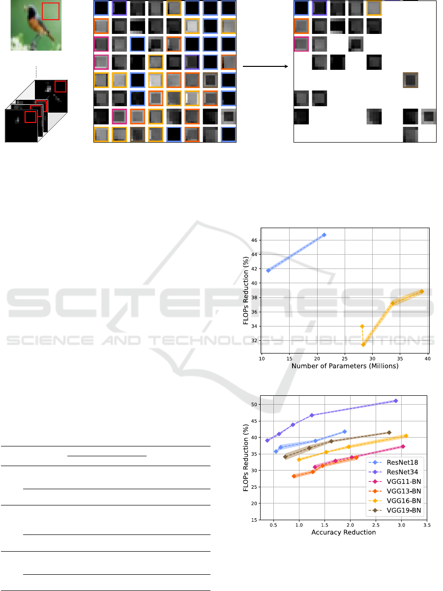
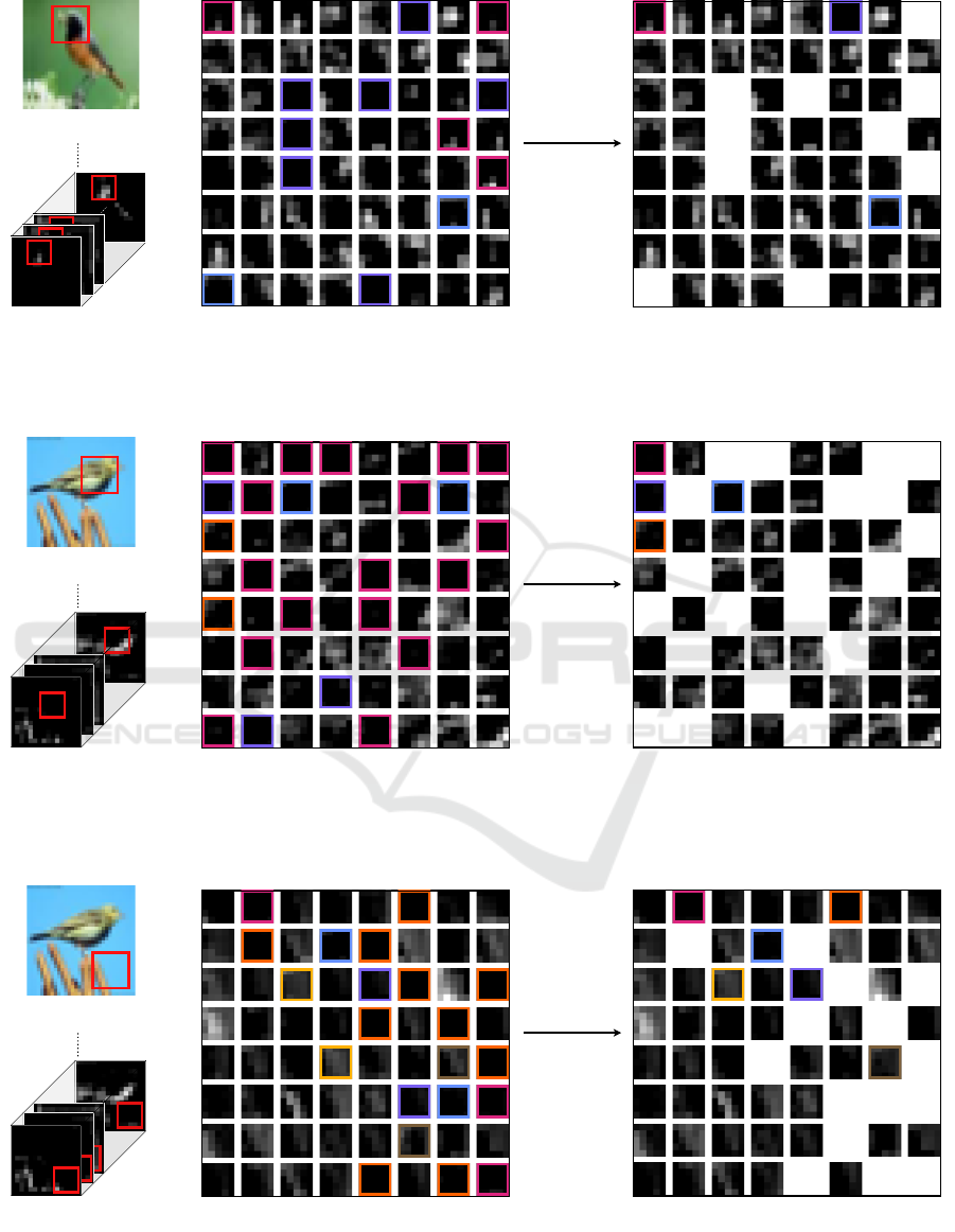
Figure 3: Visualization of the input channel compression performed by the HASTE module in a ResNet18 model on CIFAR-10.
One observed patch is marked as a red square on the input feature maps. All 64 channels of this patch are then plotted in an
8 × 8 grid. Patches with identical hash codes receive identical outline colors and are averaged by taking their mean. Patches
with no matching hash code are left unchanged. Here, we reduce the input channel dimension from 64 to 24 , which gives us a
compression ratio of r = 62.50%.
targeted cost reduction and retained accuracy is influ-
enced by the choice of L . Increased accuracy on the
test set, achieved by increasing L , is directly related
to less FLOPs reduction. For instance, we can vary
the accuracy loss on ResNet34 between 2.89 ( L = 12 )
and 0.38 ( L = 20 ) percentage points to achieve 51.09%
and 39.07% reduction in FLOPs, respectively.
We also give an overview of results from related
approaches in Table 2. Although our method is not
trained or fine-tuned on the dataset, it achieves compa-
rable results to approaches which tailored their pruning
scheme to the data. Specifically, for the ResNet18 and
VGG19-BN models, our method is on par with the best
trained approaches, namely DMCP (Xu et al., 2021)
and SSL (Wen et al., 2016), achieving a similar ratio
of FLOPs reduction to retained accuracy.
Table 2: Selected results on CIFAR-10. ”FLOPs Red.” de-
notes the percentage decrease of FLOPs after pruning com-
pared to the base model.
Model Method
Top-1 Accuracy (%)
FLOPs Red.
(%)
Data-
Free
Baseline Pruned ∆
ResNet18
PFEC
∗
91.38 89.63 1.75 11.71 ✗
SSL
∗
92.79 92.45 0.34 14.69 ✗
DMCP 92.87 92.61 0.26 35.27 ✗
Ours (L = 14) 93.07 91.18 (±0.38) 1.89 41.75 (±0.28) ✓
Ours (L = 20) 93.07 92.52 (±0.10) 0.55 35.73 (±0.09) ✓
VGG16-BN
PFEC
∗
91.85 91.29 0.56 13.89 ✗
SSL
∗
92.09 91.80 0.29 17.76 ✗
DMCP 92.21 92.04 0.17 25.05 ✗
FTWT 93.82 93.73 0.09 44.00 ✗
Ours (L = 18) 94.00 92.03 (±0.21) 1.97 37.15 (±0.47) ✓
Ours (L = 22) 94.00 93.00 (±0.12) 1.00 33.25 (±0.44) ✓
VGG19-BN
PFEC
∗
92.11 91.78 0.33 16.55 ✗
SSL
∗
92.02 91.60 0.42 30.68 ✗
DMCP 92.19 91.94 0.25 34.14 ✗
Ours (L = 18) 93.95 92.32 (±0.35) 1.63 38.83 (±0.36) ✓
Ours (L = 22) 93.95 93.22 (±0.14) 0.73 34.11 (±0.99) ✓
*
Results taken from Xu et al. (2021).
ResNet18
ResNet34
VGG11-BN
VGG13-BN
VGG16-BN
VGG19-BN
(a) Overview of CIFAR-10 results.
12
14
16
14
16
16
18
18
20
18
20
20
22
16
18
20
22
18
20
22
24
18
20
22
24
(b) Influence of hyperparameter L.
Figure 4: Results of our method on the CIFAR-10 dataset. (a)
shows the achieved FLOPs reduction for all tested models,
using L = 14 for ResNets and L = 20 for VGG-BN models.
(b) depicts the influence of the chosen number of hyperplanes
L (shown in gray) on compression rates and accuracy.
VISAPP 2025 - 20th International Conference on Computer Vision Theory and Applications
202

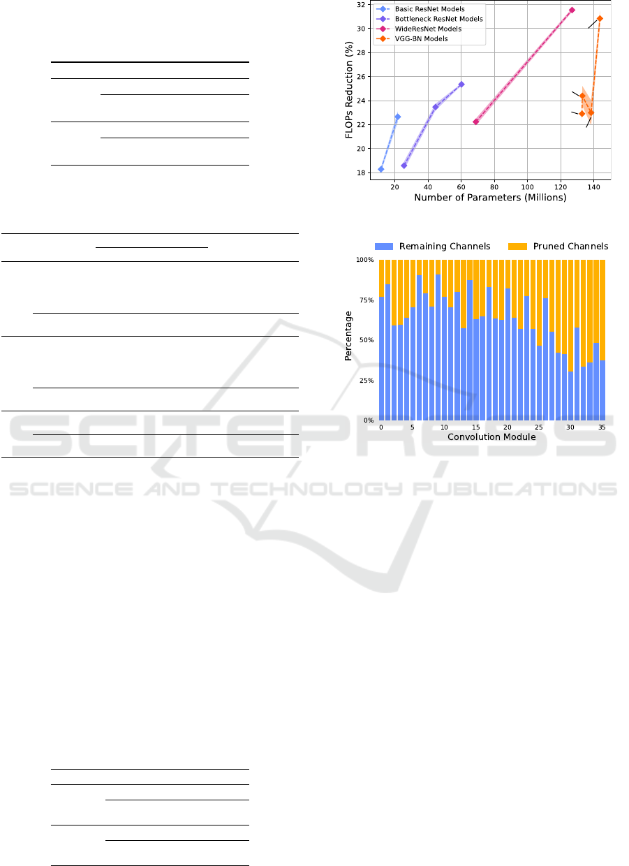
Table 3: Latency estimates for the HASTE module on
CIFAR-10. The realistic setting assumes hardware support
for efficient patch-wise operations. The theoretical speedup
is derived from the achieved FLOPs reduction.
Model Setting Latency Speedup
ResNet18
(L = 14)
Baseline 8.73ms /
Realistic 5.88ms 1.48x
Theoretical 5.09ms 1.72x
ResNet34
(L = 14)
Baseline 15.54 ms /
Realistic 10.60 ms 1.47x
Theoretical 8.28 ms 1.88x
Table 4: Selected results on ImageNet. ”FLOPs Red.” de-
notes the percentage reduction of FLOPs after pruning com-
pared to the baseline.
Model Method
Top-1 Accuracy (%)
FLOPs Red.
(%)
Data-
Free
Baseline Pruned ∆
ResNet18
LCCN 69.98 66.33 3.65 34.60 ✗
DynConv
∗
69.76 66.97 2.79 41.50 ✗
FPGM 70.28 68.34 1.94 41.80 ✗
FBS 70.71 68.17 2.54 49.49 ✗
FTWT 69.76 67.49 2.27 51.56 ✗
Ours (L = 16) 69.76 66.97 (±0.21) 2.79 18.28 (±0.19) ✓
Ours (L = 20) 69.76 68.64 (±0.56) 1.12 15.10 (±0.18) ✓
ResNet34
PFEC 73.23 72.09 1.14 24.20 ✗
LCCN 73.42 72.99 0.43 24.80 ✗
FPGM 73.92 72.54 1.38 41.10 ✗
FTWT 73.30 72.17 1.13 47.42 ✗
DGNet 73.31 71.95 1.36 67.20 ✗
Ours (L = 16) 73.31 70.31 (±0.07) 3.00 22.65 (±0.45) ✓
Ours (L = 20) 73.31 72.06 (±0.05) 1.25 18.69 (±0.30) ✓
ResNet50
FPGM 76.15 74.83 1.32 53.50 ✗
DGNet 76.13 75.12 1.01 67.90 ✗
Ours (L = 28) 76.13 73.04 (±0.07) 3.09 18.58 (±0.33) ✓
Ours (L = 36) 76.13 74.77 (±0.10) 1.36 15.68 (±0.16) ✓
*
Results taken from Li et al. (2021).
4.3 Results on ImageNet
On the ImageNet benchmark dataset, we evaluate all
available ResNet architectures including WideResNets
as well as all VGG-BN models. Results are presented
in Figures 5a and 5b. In particular, we observe a
positive scaling behavior of our method in Figure
5a, achieving up to 31.54% FLOPs reduction for a
WideResNet101. When observing models of similar
architecture, the potential FLOPs reduction grows with
the number of parameters. We relate this to the fact
that larger models typically exhibit more redundancies,
Table 5: Latency estimates for the HASTE module on Im-
ageNet. The realistic setting assumes hardware support for
efficient patch-wise operations. The theoretical speedup is
derived from the achieved FLOPs reduction.
Model Setting Latency Speedup
ResNet34
(L = 16)
Baseline 103.50 ms /
Realistic 84.56 ms 1.22x
Theoretical 80.06ms 1.29x
VGG19-BN
(L = 20)
Baseline 476.96 ms /
Realistic 371.59 ms 1.28x
Theoretical 329.91 ms 1.45x
ResNet18
ResNet50
ResNet34
ResNet101
ResNet152
WideResNet50
WideResNet101
VGG11-BN
VGG13-BN
VGG16-BN
VGG19-BN
(a) Overview of ImageNet experiments.
(b) Distribution of pruned channels in a ResNet50.
Figure 5: Visualization of results on the ImageNet dataset.
(a) depicts the relation of FLOPs reduction to number of
parameters for all tested architectures. Results are shown
with L = 16 for basic ResNet models, L = 28 for bottleneck
ResNets, L = 32 for WideResNets, and L = 20 for VGG-
BN models. (b) shows the achieved compression rate per
convolution module in a ResNet50, starting from the second
bottleneck layer.
which are then compressed by our module.
Similar to He et al. (2018), we observe that models
including pointwise convolutions are harder to prune
than their counterparts which rely solely on larger filter
kernels. This is particularly apparent in the drop in
FLOPs reduction from ResNet34 to ResNet50. While
the larger ResNet and WideResNet models with bottle-
neck blocks continue the scaling pattern, the introduc-
tion of pointwise convolutions momentarily dampens
the computational cost reduction. Increasing the width
of each convolutional layer benefits pruning perfor-
mance, as is apparent with the results of WideRes-
Net50 with twice the number of channels per layer
as in ResNet50. While pointwise convolutions can
achieve similar or even better compression ratios com-
pared to 3 × 3 convolutions (see Figure 5b), the cost
overhead of the hashing and merging steps is higher
Data-Free Dynamic Compression of CNNs for Tractable Efficiency
203

relative to the baseline.
When comparing the results to those on CIFAR-
10, we note that our HASTE module achieves less
compression on ImageNet classifiers. We directly re-
late this to the higher complexity in the data. With
a 100-fold increase in number of classes and roughly
26 times more training images than on CIFAR-10, the
models store more information in latent feature maps,
rendering them less redundant and therefore harder to
compress. Methods that exploit training data for exten-
sively tuning their pruning scheme naturally achieve
higher degrees of FLOPs reduction, as shown in Table
4. However, this is only possible when access to the
data is granted. In contrast, our method offers sig-
nificant reductions of computational cost while being
data-free, even scaling with larger model architectures.
5 CONCLUSION
While existing channel pruning approaches rely on
training data to achieve notable reductions in compu-
tational cost, our proposed HASTE module removes
restrictive requirements on data availability and com-
presses CNNs without requiring any training steps. By
employing a locality-sensitive hashing scheme for re-
dundancy detection, we are able to drastically reduce
the depth of latent feature maps and corresponding con-
volutional filters to significantly decrease the model’s
total FLOPs requirement. Our approach prunes the
model at runtime in an input-dependent manner, even
allowing for changes to the compression ratio in real
time. This property could be particularly suitable in a
federated learning scenario, where the model’s weights
are continuously updated, rendering other pruning
methods which require pre-processing of the model’s
weights infeasible.
We empirically validate our claim through a se-
ries of experiments with a variety of CNN models and
achieve compelling results on the CIFAR-10 and Im-
ageNet benchmark datasets. We aim for our method
to serve as an initial step in the direction of entirely
data-free methods for on-the-fly compression of con-
volutional architectures. Future work involves the in-
tegration of our method into related computer vision
tasks and its extension to novel architectures.
REFERENCES
Achlioptas, D. (2003). Database-friendly random projec-
tions: Johnson-Lindenstrauss with binary coins. Jour-
nal of Computer and System Sciences, 66(4):671–687.
Special Issue on PODS 2001.
Anwar, S., Hwang, K., and Sung, W. (2017). Structured
Pruning of Deep Convolutional Neural Networks. J.
Emerg. Technol. Comput. Syst., 13(3).
Bai, S., Chen, J., Shen, X., Qian, Y., and Liu, Y. (2023). Uni-
fied Data-Free Compression: Pruning and Quantization
without Fine-Tuning. In Proceedings of the IEEE/CVF
International Conference on Computer Vision (ICCV),
pages 5876–5885.
Bejnordi, B. E., Blankevoort, T., and Welling, M. (2020).
Batch-Shaping for Learning Conditional Channel
Gated Networks. In International Conference on
Learning Representations.
Belcak, P. and Wattenhofer, R. (2023). Exponen-
tially Faster Language Modelling. arXiv preprint
arXiv:2311.10770.
Chen, B., Liu, Z., Peng, B., Xu, Z., Li, J. L., Dao, T., Song,
Z., Shrivastava, A., and Re, C. (2021). MONGOOSE:
A Learnable LSH Framework for Efficient Neural Net-
work Training. In International Conference on Learn-
ing Representations.
Chen, B., Medini, T., Farwell, J., Gobriel, S., Tai, C., and
Shrivastava, A. (2020). SLIDE : In Defense of Smart
Algorithms over Hardware Acceleration for Large-
Scale Deep Learning Systems. In Proceedings of Ma-
chine Learning and Systems, volume 2, pages 291–306.
Dong, X., Huang, J., Yang, Y., and Yan, S. (2017). More is
Less: A More Complicated Network with Less Infer-
ence Complexity. In 2017 IEEE Conference on Com-
puter Vision and Pattern Recognition (CVPR), pages
1895–1903, Los Alamitos, CA, USA. IEEE Computer
Society.
Dosovitskiy, A., Beyer, L., Kolesnikov, A., Weissenborn, D.,
Zhai, X., Unterthiner, T., Dehghani, M., Minderer, M.,
Heigold, G., Gelly, S., Uszkoreit, J., and Houlsby, N.
(2021). An Image is Worth 16x16 Words: Transform-
ers for Image Recognition at Scale. In International
Conference on Learning Representations.
Elkerdawy, S., Elhoushi, M., Zhang, H., and Ray, N. (2022).
Fire Together Wire Together: A Dynamic Pruning Ap-
proach with Self-Supervised Mask Prediction. In 2022
Proceedings of the IEEE/CVF Conference on Com-
puter Vision and Pattern Recognition (CVPR), pages
12444–12453.
Gao, X., Zhao, Y., Ł ukasz Dudziak, Mullins, R., and Xu,
C.-Z. (2019). Dynamic Channel Pruning: Feature
Boosting and Suppression. In International Conference
on Learning Representations.
Goodfellow, I. J., Mirza, M., Da, X., Courville, A. C., and
Bengio, Y. (2014). An Empirical Investigation of Catas-
trophic Forgeting in Gradient-Based Neural Networks.
In Bengio, Y. and LeCun, Y., editors, 2nd International
Conference on Learning Representations, ICLR 2014,
Banff, AB, Canada, April 14-16, 2014, Conference
Track Proceedings.
Han, K., Wang, Y., Tian, Q., Guo, J., Xu, C., and Xu, C.
(2020). GhostNet: More Features From Cheap Oper-
ations. In 2020 IEEE/CVF Conference on Computer
Vision and Pattern Recognition (CVPR), pages 1577–
1586.
He, K., Zhang, X., Ren, S., and Sun, J. (2016). Deep Resid-
ual Learning for Image Recognition. In 2016 IEEE
VISAPP 2025 - 20th International Conference on Computer Vision Theory and Applications
204

Conference on Computer Vision and Pattern Recogni-
tion (CVPR), pages 770–778.
He, Y., Lin, J., Liu, Z., Wang, H., Li, L.-J., and Han, S.
(2018). AMC: AutoML for Model Compression and
Acceleration on Mobile Devices. In Ferrari, V., Hebert,
M., Sminchisescu, C., and Weiss, Y., editors, Computer
Vision – ECCV 2018, pages 815–832, Cham. Springer
International Publishing.
He, Y., Liu, P., Wang, Z., Hu, Z., and Yang, Y. (2019). Filter
Pruning via Geometric Median for Deep Convolutional
Neural Networks Acceleration. In 2019 IEEE/CVF
Conference on Computer Vision and Pattern Recogni-
tion (CVPR), pages 4335–4344.
Howard, A., Zhu, M., Chen, B., Kalenichenko, D., Wang,
W., Weyand, T., Andreetto, M., and Adam, H. (2017).
MobileNets: Efficient Convolutional Neural Networks
for Mobile Vision Applications. arXiv preprint
arXiv:1704.04861.
Hua, W., Zhou, Y., De Sa, C., Zhang, Z., and Suh, G. E.
(2019). Channel Gating Neural Networks. In Advances
in Neural Information Processing Systems, volume 32,
Red Hook, NY, USA. Curran Associates Inc.
Indyk, P. and Motwani, R. (1998). Approximate Nearest
Neighbors: Towards Removing the Curse of Dimen-
sionality. In Proceedings of the Thirtieth Annual ACM
Symposium on Theory of Computing, STOC ’98, page
604–613, New York, NY, USA. Association for Com-
puting Machinery.
Kitaev, N., Kaiser, L., and Levskaya, A. (2020). Reformer:
The Efficient Transformer. In International Conference
on Learning Representations.
Krizhevsky, A. (2009). Learning Multiple Layers of Features
from Tiny Images.
Li, F., Li, G., He, X., and Cheng, J. (2021). Dynamic
Dual Gating Neural Networks. In 2021 IEEE/CVF
International Conference on Computer Vision (ICCV),
pages 5310–5319.
Li, H., Kadav, A., Durdanovic, I., Samet, H., and Graf, H. P.
(2017). Pruning Filters for Efficient ConvNets. In In-
ternational Conference on Learning Representations.
Li, P., Hastie, T., and Church, K. (2006). Very Sparse Ran-
dom Projections. In Proceedings of the 12th ACM
SIGKDD International Conference on Knowledge Dis-
covery and Data Mining, volume 2006 of KDD ’06,
pages 287–296.
Lin, J., Rao, Y., Lu, J., and Zhou, J. (2017a). Runtime
Neural Pruning. In Guyon, I., Luxburg, U. V., Bengio,
S., Wallach, H., Fergus, R., Vishwanathan, S., and
Garnett, R., editors, Advances in Neural Information
Processing Systems, volume 30. Curran Associates,
Inc.
Lin, X., Zhao, C., and Pan, W. (2017b). Towards Accurate
Binary Convolutional Neural Network. In Proceed-
ings of the 31st International Conference on Neural
Information Processing Systems, pages 344–352.
Liu, L., Deng, L., Hu, X., Zhu, M., Li, G., Ding, Y., and Xie,
Y. (2019). Dynamic Sparse Graph for Efficient Deep
Learning. In International Conference on Learning
Representations.
Liu, Z., Coleman, B., and Shrivastava, A. (2021a). Ef-
ficient Inference via Universal LSH Kernel. CoRR,
abs/2106.11426.
Liu, Z., Li, J., Shen, Z., Huang, G., Yan, S., and Zhang, C.
(2017). Learning Efficient Convolutional Networks
through Network Slimming. In 2017 IEEE Interna-
tional Conference on Computer Vision (ICCV), pages
2755–2763, Los Alamitos, CA, USA. IEEE Computer
Society.
Liu, Z., Lin, Y., Cao, Y., Hu, H., Wei, Y., Zhang, Z., Lin, S.,
and Guo, B. (2021b). Swin Transformer: Hierarchical
Vision Transformer using Shifted Windows. In 2021
IEEE/CVF International Conference on Computer Vi-
sion (ICCV), pages 9992–10002. IEEE Computer So-
ciety.
Liu, Z., Mao, H., Wu, C. Y., Feichtenhofer, C., Darrell, T.,
and Xie, S. (2022). A ConvNet for the 2020s. In Pro-
ceedings of the IEEE/CVF Conference on Computer Vi-
sion and Pattern Recognition (CVPR), Proceedings of
the IEEE Computer Society Conference on Computer
Vision and Pattern Recognition, pages 11966–11976.
IEEE Computer Society.
Liu, Z., Wang, P., and Li, Z. (2021c). More-Similar-Less-
Important: Filter Pruning VIA Kmeans Clustering. In
2021 IEEE International Conference on Multimedia
and Expo (ICME), pages 1–6.
Luo, J., Wu, J., and Lin, W. (2017). ThiNet: A Filter Level
Pruning Method for Deep Neural Network Compres-
sion. In IEEE International Conference on Computer
Vision, ICCV 2017, Venice, Italy, October 22-29, 2017,
pages 5068–5076. IEEE Computer Society.
Ma, N., Zhang, X., Zheng, H.-T., and Sun, J. (2018). Shuf-
fleNet V2: Practical Guidelines for Efficient CNN
Architecture Design. In Computer Vision – ECCV
2018: 15th European Conference, Munich, Germany,
September 8–14, 2018, Proceedings, Part XIV, pages
122––138.
M
¨
uller, T., Evans, A., Schied, C., and Keller, A. (2022).
Instant Neural Graphics Primitives with a Multiresolu-
tion Hash Encoding. ACM Trans. Graph., 41(4):102:1–
102:15.
Paszke, A., Gross, S., Massa, F., Lerer, A., Bradbury, J.,
Chanan, G., Killeen, T., Lin, Z., Gimelshein, N.,
Antiga, L., Desmaison, A., K
¨
opf, A., Yang, E., DeVito,
Z., Raison, M., Tejani, A., Chilamkurthy, S., Steiner,
B., Fang, L., Bai, J., and Chintala, S. (2019). PyTorch:
An Imperative Style, High-Performance Deep Learn-
ing Library.
Phan, H. (2021). PyTorch models trained on CIFAR-
10 dataset. https://github.com/huyvnphan/PyTorch
CIFAR10.
Pleiss, G., Chen, D., Huang, G., Li, T., van der Maaten,
L., and Weinberger, K. Q. (2017). Memory-Efficient
Implementation of DenseNets. CoRR, abs/1707.06990.
Russakovsky, O., Deng, J., Su, H., Krause, J., Satheesh, S.,
Ma, S., Huang, Z., Karpathy, A., Khosla, A., Bernstein,
M., Berg, A., and Fei-Fei, L. (2015). ImageNet Large
Scale Visual Recognition Challenge. International
Journal of Computer Vision, 115(3):211–252.
Sandler, M., Howard, A., Zhu, M., Zhmoginov, A., and
Data-Free Dynamic Compression of CNNs for Tractable Efficiency
205

Chen, L.-C. (2018). MobileNetV2: Inverted Residu-
als and Linear Bottlenecks. In 2018 IEEE/CVF Con-
ference on Computer Vision and Pattern Recognition
(CVPR), pages 4510–4520, Los Alamitos, CA, USA.
IEEE Computer Society.
Simonyan, K. and Zisserman, A. (2015). Very Deep Convo-
lutional Networks for Large-Scale Image Recognition.
In International Conference on Learning Representa-
tions.
Tan, M. and Le, Q. (2019). EfficientNet: Rethinking Model
Scaling for Convolutional Neural Networks. In Chaud-
huri, K. and Salakhutdinov, R., editors, Proceedings of
the 36th International Conference on Machine Learn-
ing, volume 97 of Proceedings of Machine Learning
Research, pages 6105–6114. PMLR.
Tan, M. and Le, Q. (2021). EfficientNetV2: Smaller Mod-
els and Faster Training. In Meila, M. and Zhang, T.,
editors, Proceedings of the 38th International Confer-
ence on Machine Learning, volume 139 of Proceedings
of Machine Learning Research, pages 10096–10106.
PMLR.
Verelst, T. and Tuytelaars, T. (2020). Dynamic Convolutions:
Exploiting Spatial Sparsity for Faster Inference. In
2020 IEEE/CVF Conference on Computer Vision and
Pattern Recognition (CVPR), pages 2317–2326, Los
Alamitos, CA, USA. IEEE Computer Society.
Wen, W., Wu, C., Wang, Y., Chen, Y., and Li, H. (2016).
Learning Structured Sparsity in Deep Neural Networks.
In Proceedings of the 30th International Conference
on Neural Information Processing Systems, NIPS’16,
page 2082–2090. Curran Associates Inc.
Wimmer, P., Mehnert, J., and Condurache, A. P. (2023). Di-
mensionality reduced training by pruning and freezing
parts of a deep neural network: a survey. Artificial
Intelligence Review.
Woo, S., Debnath, S., Hu, R., Chen, X., Liu, Z., Kweon,
I. S., and Xie, S. (2023). ConvNeXt V2: Co-Designing
and Scaling ConvNets With Masked Autoencoders. In
Proceedings of the IEEE/CVF Conference on Com-
puter Vision and Pattern Recognition (CVPR), pages
16133–16142.
Xu, Z., Sun, J., Liu, Y., and Sun, G. (2021). An Efficient
Channel-level Pruning for CNNs without Fine-tuning.
In 2021 International Joint Conference on Neural Net-
works (IJCNN), pages 1–8.
Yin, H., Molchanov, P., Alvarez, J. M., Li, Z., Mallya, A.,
Hoiem, D., Jha, N. K., and Kautz, J. (2020). Dreaming
to Distill: Data-free Knowledge Transfer via Deepin-
version. In Proceedings of the IEEE/CVF Conference
on Computer Vision and Pattern Recognition, pages
8715–8724.
Yvinec, E., Dapogny, A., Cord, M., and Bailly, K. (2023).
RED++ : Data-Free Pruning of Deep Neural Networks
via Input Splitting and Output Merging. IEEE Trans-
actions on Pattern Analysis & Machine Intelligence,
45(03):3664–3676.
Zhang, X., Zhou, X., Lin, M., and Sun, J. (2018). Shufflenet:
An extremely efficient convolutional neural network
for mobile devices. In Proceedings of the IEEE Con-
ference on Computer Vision and Pattern Recognition
(CVPR).
Zhang, X., Zou, J., He, K., and Sun, J. (2016). Accelerating
Very Deep Convolutional Networks for Classification
and Detection. IEEE Transactions on Pattern Analysis
and Machine Intelligence, 38(10):1943–1955.
Zhuang, Z., Tan, M., Zhuang, B., Liu, J., Guo, Y., Wu,
Q., Huang, J., and Zhu, J. (2018). Discrimination-
Aware Channel Pruning for Deep Neural Networks.
In Proceedings of the 32nd International Conference
on Neural Information Processing Systems, NIPS’18,
page 883–894.
APPENDIX
Latency Considerations
While many pruning approaches focus on generating
small but dense models that are easy to execute, it
is also possible to achieve significant latency bene-
fits using methods that leverage non-contiguous sets
of weights which are chosen in an input-dependent
manner (Chen et al., 2020, 2021; Kitaev et al., 2020;
Belcak and Wattenhofer, 2023). Our HASTE module
employs a similar technique by only computing the
convolution on non-redundant channels.
However, modern deep learning frameworks do not
support conditional execution operations natively (Bel-
cak and Wattenhofer, 2023) and are optimized towards
large, dense matrix multiplications, as is the case with
PyTorch (Paszke et al., 2019). Thus, highly optimized
implementations are necessary to allow conditional
execution strategies to compete with dense models.
We focus our efforts on providing a proof of concept
for the viability of dynamic, data-free pruning in Py-
Torch due to its wide-spread use in machine learning
research.
For the latency estimates shown in Tables 3 and 5
of the main text, we present two different scenarios:
• Realistic. In this scenario, we assume that the hard-
ware is capable of handling patch-wise varying
channel depths. This allows for accurate execution
of our proposed method, as different compression
ratios per patch can be fully utilized.
• Theoretical. In the theoretical setting, we assume
that the latency of the baseline model is reduced
by the same amount as the reduction in FLOPs, as
observed in our experiments.
In both scenarios, we measure the total latency per im-
age of the model equipped with our proposed HASTE
modules, across a batch of 64 images from the respec-
tive dataset. Since the PyTorch framework does not
support efficient computations with ternary weights
{−1,0, 1} as required for our hashing scheme, we ex-
trapolate its latency based on the FLOPs count.
VISAPP 2025 - 20th International Conference on Computer Vision Theory and Applications
206

Table 6: Overview of experiments for the data-free L
1
norm-
based pruning baseline. ”Usage of Patches” denotes whether
the pruning is applied to an entire input channel ( ✗ ), or
individually for each channel of each patch ( ✓ ), as visualized
in Figure 2 of the main text. ”Pruning Criterion” indicates
whether the L
1
norm of channels or locality-sensitive hashing
(LSH) is used to determine which channels to prune. Lastly,
”Pruning Operation” denotes if the selected channels are
removed or merged into one singular channel.
Prune Merge Patch-Prune Patch-Merge Ours
(P) (M) (PP) (PM) (HASTE)
Usage of Patches ✗ ✗ ✓ ✓ ✓
Pruning Criterion L
1
L
1
L
1
L
1
LSH
Pruning Operation Remove Merge Remove Merge Merge
Pruning Pointwise Convolutions
A special case of the convolution operation appears
when K = 1 . These 1 × 1 convolutions are commonly
used for downsampling or upsampling of the channel
dimension before and after parameter-heavy convolu-
tions with larger kernel sizes, or after a depth-wise
convolutional layer. However, as the kernel resolution
changes to a single pixel, each input pixel generates ex-
actly one output pixel in the spatial domain. As there
is no reduction in spatial resolution when performing
1 ×1 convolutions, we do not require the 3 ×3 patches
that rasterize the input to be overlapping. Hence, we
pad the input in such a way that each side is divisible
by 3 and use non-overlapping patches.
Component Ablation
To put the results of our LSH-based data-free com-
pression method into context, we construct an ablation
study which analyzes the impact of our method’s indi-
vidual components. As a baseline for comparison, we
employ an L
1
norm-based pruning criterion and apply
it in various settings to establish a fair comparison to
our proposed HASTE module. For all experiments
we compute the L
1
norm of channels of the input fea-
ture maps of convolution modules and prune a fixed
percentage of channels with the lowest norm (see (Li
et al., 2017)) to achieve comparable FLOPs reductions
to the HASTE module.
The results are presented in Tables 6 and 7. At a
given compression ratio, the L
1
norm-based pruning
approaches do not keep the pruned model’s accuracy at
an acceptable level. In contrast, the proposed HASTE
module is able to keep near-baseline accuracy.
Visualizations
To gain an intuitive understanding of the merge opera-
tion for redundant feature map channels as described
Table 7: Comparison of results of data-free L
1
norm-based
pruning methods (see Table 6) to our proposed HASTE mod-
ule on the CIFAR-10 dataset. ”FLOPs Red.” denotes the
percentage decrease of FLOPs after pruning compared to the
base model. We highlight the highest remaining Top-1 accu-
racy and lowest loss of accuracy ( ∆ ) for each compression
target in bold.
Model Method
Top-1 Accuracy (%)
FLOPs
Reduction (%)
Baseline Pruned ∆
ResNet18
P 93.07 71.07 22.00 40.80
M 93.07 65.31 27.76 41.75
PP 93.07 88.70 4.37 40.80
PM 93.07 86.53 6.54 39.89
HASTE 93.07 91.18 1.89 41.75
ResNet34
P 93.34 48.42 44.92 51.98
M 93.34 40.52 52.82 53.13
PP 93.34 80.04 13.30 51.98
PM 93.34 72.10 21.24 50.51
HASTE 93.34 90.45 2.89 51.09
VGG11-BN
P 92.39 41.77 50.62 37.87
M 92.39 73.87 18.52 38.90
PP 92.39 65.94 25.45 37.87
PM 92.39 87.39 5.00 37.11
HASTE 92.39 89.36 3.03 37.25
VGG19-BN
P 93.95 34.89 59.06 40.73
M 93.95 42.23 51.72 42.02
PP 93.95 65.84 28.11 40.72
PM 93.95 82.51 11.44 40.31
HASTE 93.95 91.19 2.76 41.47
in Section 3.3 of the main text, we provide visualiza-
tions of the latent features before and after the merging
step in Figures 3, 6, 7 and 8. Note that the compres-
sion ratio r = 1 − (
˜
C
in
/C
in
) ∈ (0, 1) changes not only
depending on the input image, but on the amount of
redundancies found in each individual patch. The
comparison of Figures 3 and 6 reveal an interesting
property of our proposed HASTE module: Patches
that contain little class-specific information, such as
the background, can be compressed to a much higher
degree than patches that contain relevant information
for the classification task.
Data-Free Dynamic Compression of CNNs for Tractable Efficiency
207

Latent Feature Map Detected Redundancies in Patches Extracted
from Feature Map
Compute Mean
per Bucket
Patch Projected
onto Input Image
Remaining Channels after Merging Redundancies
Figure 6: Visualization of the input channel compression performed by the HASTE module. Patches with identical hash codes
receive identical outline colors and are averaged by taking their mean. Patches with no matching hash code are left unchanged.
Here, we reduce C
in
= 64 to
˜
C
in
= 54, which gives us a compression ratio of r = 15.63%.
Latent Feature Map Detected Redundancies in Patches Extracted
from Feature Map
Compute Mean
per Bucket
Patch Projected
onto Input Image
Remaining Channels after Merging Redundancies
Figure 7: Visualization of the input channel compression performed by the HASTE module. Patches with identical hash codes
receive identical outline colors and are averaged by taking their mean. Patches with no matching hash code are left unchanged.
Here, we reduce C
in
= 64 to
˜
C
in
= 44, which gives us a compression ratio of r = 31.25%.
Latent Feature Map Detected Redundancies in Patches Extracted
from Feature Map
Compute Mean
per Bucket
Patch Projected
onto Input Image
Remaining Channels after Merging Redundancies
Figure 8: Visualization of the input channel compression performed by the HASTE module. Patches with identical hash codes
receive identical outline colors and are averaged by taking their mean. Patches with no matching hash code are left unchanged.
Here, we reduce C
in
= 64 to
˜
C
in
= 49, which gives us a compression ratio of r = 23.43%.
VISAPP 2025 - 20th International Conference on Computer Vision Theory and Applications
208