Leveraging Deep Q-Network Agents with Dynamic Routing Mechanisms
in Convolutional Neural Networks for Enhanced and Reliable
Classification of Alzheimer’s Disease from MRI Scans
Jolanta Podolszanska
a
Faculty of Science & Technology, Jan Dlugosz Uniwersity, Armii Krajowej 15/17 Avenue, Czestochowa, Poland
Keywords:
CapNet, Reinforcement Learning, Agents Learning, Medical Imaging.
Abstract:
With limited data and complex image structures, accurate classification of medical images remains a significant
challenge in AI-assisted diagnostics. This study presents a hybrid CNN model with a capsule network layer
and dynamic routing mechanism, enhanced with a Deep Q-network (DQN) agent, for MRI image classification
in Alzheimer’s disease detection. The approach combines a capsule network that captures complex spatial
patterns with dynamic routing, improving model adaptability. The DQN agent manages the weights and
optimizes learning by interacting with the evolving environment. Experiments conducted on popular MRI
datasets show that the model outperforms traditional methods, significantly improving classification accuracy
and reducing misclassification rates. These results suggest that the approach has great potential for clinical
applications, contributing to the accuracy and reliability of automated diagnostic systems.
1 INTRODUCTION
Convolutional Neural Networks (CNNs) revolution-
ized computer vision by capturing spatial patterns
effectively (He et al., 2017). MRI, crucial in
Alzheimer’s disease (AD) diagnosis, detects neu-
rodegenerative changes like hippocampal atrophy
(Leszek, 2012). This work proposes a hybrid CNN-
CapsNet model with dynamic routing and a DQN
agent to enhance AD classification accuracy.
1.1 Related Works
Capsule Networks (CapsNets) effectively model hier-
archical spatial patterns, improving classification, es-
pecially in medical imaging (Sabour et al., 2017). En-
hancements like Efficient-CapsNet (Jia et al., 2022)
and Res-CapsNet (Pawan et al., 2023) use mecha-
nisms such as auto-attention and residual connections
to boost accuracy and stability. Recent applications
in Alzheimer’s (Bushara et al., 2024), lung cancer
(Bushara et al., 2024), and COVID-19 detection (Af-
shar et al., 2020) validate their utility in complex
datasets.
Techniques like SE-Inception-ResNet (Xi et al.,
2023) and TE-CapsNet (Yadav and Dhage, 2024) ad-
a
https://orcid.org/0000-0002-6032-5654
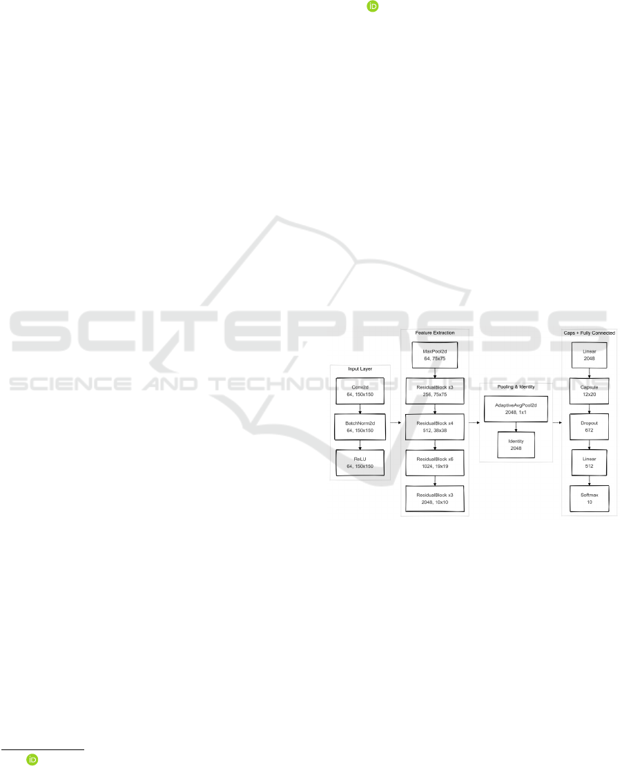
Figure 1: CNN Architecture diagram.
dress challenges such as class imbalance and compu-
tational costs. MResCaps (Abhishek et al., 2024) and
S-VCNet effectively classify datasets like DermaM-
NIST and OrganMNIST-S, demonstrating the versa-
tility of CapsNets.
Reinforcement learning-based dynamic routing
improves adaptability in tasks like Alzheimer’s dis-
ease progression analysis (Jiao and et al., 2019),
malaria detection (Madhu et al., 2021), and lung
cancer classification in CT images (Bushara et al.,
2024). Combining pre-trained ResNet weights with
CapsNets enables robust spatial feature analysis and
accurate diagnostic predictions.
1172
Podolszanska, J.
Leveraging Deep Q-Network Agents with Dynamic Routing Mechanisms in Convolutional Neural Networks for Enhanced and Reliable Classification of Alzheimer’s Disease from MRI Scans.
DOI: 10.5220/0013301900003890
Paper published under CC license (CC BY-NC-ND 4.0)
In Proceedings of the 17th International Conference on Agents and Artificial Intelligence (ICAART 2025) - Volume 3, pages 1172-1179
ISBN: 978-989-758-737-5; ISSN: 2184-433X
Proceedings Copyright © 2025 by SCITEPRESS – Science and Technology Publications, Lda.

2 NETWORK ARCHITECTURE
The efficiency of machine learning systems re-
lies on their architecture. This section details the
model’s structure, parameters, and optimization tech-
niques designed to enhance accuracy and perfor-
mance. Unique features distinguish it from conven-
tional methods, contributing to its superior results.
2.1 Dynamic Routing
Some decisions, like recognizing large objects, are
simpler than specialized tasks requiring domain
knowledge. Complex tasks benefit from systems that
identify subtasks and select suitable algorithms. Re-
search (Jiao and et al., 2019), (Madhu et al., 2021),
(Bushara et al., 2024) shows dynamic routing im-
proves accuracy but often neglects computational
costs, relying on opaque heuristics for efficiency. This
approach leverages ResNet-50.
In dynamic routing, let b
i j
∈R represent the initial
coefficient, signifying the “belief” of input capsule i
about contributing to output capsule j. Initially, b
i j
in-
dicates no prediction for any output capsule. During
routing, these coefficients are iteratively updated to
optimize the correspondence between input and out-
put capsules, as defined in (1).
b
i j
= b
i j
+ agreement (1)
Agreement concordance is calculated as the scalar
product of the prediction vector ˆu
i j
and the output v
j
for each capsule. Higher compatibility increases b
i j
,
which is converted to c
i j
using the softmax function
(2). In Equation (2), e is the base of the natural loga-
rithm, essential in exponential functions widely used
in machine learning.
c
i j
=
e
b
i j
∑
k
e
b
ik
(2)
Optimal routing can be modeled as a Markov de-
cision process (Bengio et al., 2015). The Q-Routing
algorithm (Bai et al., 2024), enhanced with backward
updates, improves convergence by balancing load and
energy via a reward function considering delay. Ex-
periments show it outperforms standard Q-Learning
across all metrics (Valadarsky et al., 2017). Addition-
ally, c
i j
factors summing to unity enable proportional
activation allocation to output capsules based on pre-
diction consistency.
Routing strategy selection can be modeled as a
Markov chain. The Q-routing algorithm, enhanced
with backward updates, improves convergence and
optimizes routing by balancing load and energy
through a reward function. It outperforms Q-Learning
across metrics (Valadarsky et al., 2017). The c
i j
co-
efficients ensure proportional activation allocation to
output capsules based on prediction consistency.
Let ˆu
i j
∈ R
d
be the prediction of the activation
vector from input capsule i to output capsule j. The
routing process involves iteratively assigning coeffi-
cients c
i j
∈ [0, 1] which represent the weight or con-
fidence of the input capsule i to the output capsule j.
Defined s
j
as the weighted sum of the predictions (3).
s
j
=
∑
i
c
i j
ˆu
i j
(3)
where c
i j
are calculated by applying the softmax func-
tion on b
i j
(4) values.
c
i j
=
exp(b
i j
)
∑
k
exp(b
ik
)
(4)
where b
ik
are initially initialized as zero and itera-
tively updated based on the correspondence between
the prediction ˆu
i j
and the resulting activation vector
v
j
. In each routing iteration, the value of b
i j
is up-
dated (5).
b
i j
= b
i j
+ ˆu
i j
·v
j
(5)
The scalar product ˆu
i j
·v
j
measures the correspon-
dence between the prediction ˆu
i j
and the activation
vector v
j
. When they align, b
i j
increases, boosting
the assignment factor c
i j
in subsequent iterations. It-
erative routing, performed r times, optimizes c
i j
, fo-
cusing on output capsules that aggregate input vector
predictions.
2.2 Simulation of a Capsule-Based
Environment
The capsule network in this work employs a Dy-
namic Routing Capsule Layer inspired by (Sabour
et al., 2017). This layer utilizes iterative routing-by-
agreement to determine the contributions of lower-
level capsules to higher-level capsule outputs. A
squashing function ensures vector normalization
and learnable transformation matrices are used for
capsule-to-capsule predictions.
Consider an agent learning environment as a
single-step decision-making process that can be mod-
elled as a Markov process. The agent selects an output
capsule in the decision environment to maximize the
reward function. The state space S, where s ∈ S, is
represented as the activation vector of the input cap-
sules (6).
s = [a
1
, a
2
, a
3
, ..., ∈ R
C
in
] (6)
The activation of input capsule i, denoted as a
i
, is ran-
domly initialized at the start of training, making the
Leveraging Deep Q-Network Agents with Dynamic Routing Mechanisms in Convolutional Neural Networks for Enhanced and Reliable
Classification of Alzheimer’s Disease from MRI Scans
1173

state s a random vector. An agent selects an action
a ∈ A, where A = {1, 2, 3, . . . ,C
out
}, representing the
selection of one output capsule from C
out
. The reward
function R(s,a) is defined as the return value and is
currently random (7).
R(s, a) = random ∼U(0, 1) (7)
where U(0, 1) for uniform distribution. In the fu-
ture, an extended feature may be available that will be
based on state-to-state correspondence, and the fea-
ture may be available as an early activation and actual
output capsule feature. At the beginning of the sec-
tion, the state is randomly initialized (8)
s = [a
1
, a
2
, . . . , a
C
in
], a
i
∼ N (0, 1) (8)
where N (0, 1) is a normal distribution with expected
value 0 and variance 1. The agent chooses action
a ∈ A, which represents the choice of output capsule.
After action a is executed, state s is re-initialized(9).
s
′
= [a
′
1
, a
′
2
, . . . , a
′
C
in
], a
′
i
∼ N (0, 1) (9)
In the future, this environment will be extended to al-
low the software to deal with more complex classifi-
cations.
2.3 Agent Model
The agent model approximates action values Q(s, a)
as in the Deep Q-Learning (DQN) algorithm. The
state s ∈ R
d
represents the environment, where d
s
is
the state space dimension. The action a ∈ A, with
A = {1, 2, 3, . . . , d
a
}, belongs to a finite action space
of size d
a
. The network aims to approximate Q(s, a),
the expected cumulative reward for taking action a in
state s (10).
Q(s, a) = E
"
∞
∑
t=0
γ
t
r
t
| s
0
= s, a
0
= a
#
(10)
where r
t
is the reward at step t, and γ ∈[0, 1) is the dis-
count factor. The agent approximates the value func-
tion Q(s, a) using a neural network with three fully
connected layers. Let W
1
∈ R
128×d
s
and b
1
∈ R
128
represent the weight matrix and bias vector for the
first layer. The input vector s is transformed as fol-
lows (11).
h
1
= RELU(W
1
s + b
1
) (11)
where h
1
∈ R
128
is the output of the first layer af-
ter applying the ReLU activation function. Let W
2
∈
R
128×128
and b
2
∈R
128
be the weight matrix and bias
vector for the second layer. The transformation of the
vector h
1
is defined by the following equation(12).
h
2
= RELU(W
2
h
1
+ b
2
) (12)
where h
2
∈R
128
is the output of the second layer after
applying the ReLU activation function.
2.4 Convolutional Neural Network with
Capsule Layers
Let f (x) represent the transformation performed by
the ResNet50 network up to the Fully Connected
layer, with the output replaced by the identity func-
tion (1). After feature extraction, the result is trans-
formed by a fully connected layer to align with the
capsule layer requirements. The attention layer W
f c
∈
R
(in capsules×in dim×512)
is defined by equation (13).
z = W
f c
f (x) (13)
This result is then reshaped to the dimensions re-
quired by the capsule layer(14).
z → ˜z ∈ R
(B×in capsules×in dim)
(14)
Next, ˜z is processed by the capsule layer, which con-
verts input capsules into output capsules with spec-
ified dimensions. Using dynamic routing, the cap-
sule layer transforms ˜z ∈R
(B×in capsules×in dim)
into v ∈
R
(B×out capsules×out dim)
, as defined by equation (15).
v = CapsuleLayer(ˆz) (15)
The result is then flattened to v
flat
∈
R
(B×resnet out features+out capsules×out dim)
. The out-
put features from ResNet50 f (x) are flattened
along with the capsule layer features v
flat
, and then
combined (16).
c = Concat( f (x), v
flat
)
∈ R
(B×resnet out features+out capsules×out dim)
(16)
where c is a vector of connected features. The CNN
model uses the Focal Loss function, which is defined
by equation (17).
Focal Loss = −α(1 − p
t
)
γ
log(p
t
) (17)
where p
t
is the probability assigned to the true class.
A capsule network layer is defined as follows: let
C
in
and C
out
denote the number of input and output
capsules, respectively, and d
in
and d
out
their dimen-
sions. The capsule layer transforms x ∈ R
(B×C
in
×d
in
)
to v ∈ R
(B×C
out
×d
out
)
, where B is the batch size. The
transformation matrix W ∈ R
(1×C
in
×C
out
×d
out
×d
in
)
is a
learnable parameter. Each input vector x
i
for capsule
ICAART 2025 - 17th International Conference on Agents and Artificial Intelligence
1174

i is transformed to a prediction vector ˆu
i j
for output
capsule j using W , as defined by equation (18).
ˆu
i j
= W
i j
x
i
(18)
Prediction vectors are matched to output capsules
through an iterative routing process. The squash func-
tion normalizes output capsule vectors. Let s
j
∈ R
d
represent the output vector for capsule j, aggregated
from input capsule predictions during a routing step.
The squash function transforms s
j
into v
j
with a norm
in [0, 1], defined as R
d
→ R
d
(19).
v
j
= squash(s
j
) =
∥s
j
∥
2
1 + ∥s
j
∥
2
·
s
j
∥s
j
∥+ ε
(19)
where ∥s
j
∥ denotes the Euclidean norm of the vec-
tor s
j
and ε is a small scalar value that prevents di-
vision by zero. For s
i j
= 0, we have v
i j
= 0. As the
norm ∥s
i j
∥ increases, the transformation asymptoti-
cally approaches a value close to 1 for ∥v
j
∥, allow-
ing for the amplification of activations for output cap-
sules with strong activations while suppressing cap-
sules with weak activations. This transformation is
nonlinear, which helps the model better capture de-
pendencies between input elements.
3 PROPOSED METHOD
This study optimizes Alzheimer’s disease classifica-
tion by combining capsule layers with dynamic rout-
ing (Sabour et al., 2017) and Focal Loss (Xi et al.,
2023), addressing class imbalance and preserving
spatial relationships. Dynamic routing enhances hier-
archical feature extraction, crucial in medical imaging
(Afshar et al., 2018).
Incorporating the CapsuleRoutingEnv algorithm
(Bai et al., 2024) with a DQN agent improves routing
adaptivity and precision, effectively analyzing com-
plex medical images. The model integrates ResNet,
capsule layers, attention mechanisms, and Focal Loss,
leveraging their strengths to enhance classification
(Afshar et al., 2020), (Sadeghnezhad and Salem,
2024).
3.1 Dataset
The dataset contains 6,400 MRI images, categorized
into four classes: Mild dementia (896), Moderate de-
mentia (64), Non-dementia (3,200), and Very mild de-
mentia (2,240). Images were normalized to 128x128
pixels for analysis.
3.2 Model Initialization and Initial
Configuration
The model integrates ResNet50 and CapsNet with dy-
namic routing to leverage spatial information and ad-
dress data constraints. Pre-trained ResNet weights en-
hance generalization, and reinforcement learning op-
timizes routing for improved MRI analysis.
Trained for 50 epochs with a batch size of 64, the
model used a learning rate of 0.0001, gradually in-
creased to minimize overfitting. AdamW optimizer
ensured stability and handled dynamic structures ef-
fectively.
3.3 Training and Validation Procedure
In each training iteration, the model takes a batch of
x inputs and their corresponding y labels. The goal is
to minimize the loss function L, which has been cho-
sen as Focal Loss to better deal with non-equivalent
classes. The loss value for a given batch (x, y) is cal-
culated according to the formula (17), where p
t
is the
probability assigned to the correct class (20)
p
t
=
(
p for the true class,
1 − p for the wrong class
(20)
we notice that Focal Loss value L
focal
is minimized
using the AdamW optimizer, which allows for stable
weight updates of the model. Parameters are updated
according to the gradients ∇L
focal
for each batch to
minimize the loss function.
During validation, the model is assessed for its
ability to generalize to data that was not used during
training. For each batch of validation data, the follow-
ing metrics are calculated:precision, recall, and F1.
P
i
=
T P
i
T P
i
+ FP
i
(21)
These metrics allow for the assessment of the classi-
fication quality of various data(21) and (22).
R
i
=
T P
i
T P
i
+ FN
i
(22)
where TP
i
is the number of true positive examples for
class i, FP
i
is the number of false positive examples
for class i and FN
i
is false negative examples for class
i. The F1-score for class i is calculated as the har-
monic mean of precision and recall (23).
F1
i
= 2 ·
P
i
·R
i
P
i
+ R
i
(23)
These metrics are then averaged across all classes to
produce a ”macro” score, which ensures that each
Leveraging Deep Q-Network Agents with Dynamic Routing Mechanisms in Convolutional Neural Networks for Enhanced and Reliable
Classification of Alzheimer’s Disease from MRI Scans
1175

class is treated equally regardless of its abundance in
the data. The AdamW algorithm was used to optimize
the model, which updates the weights in each iteration
under the rule (24).
θ
t+1
= θ
t
−η ·
m
t
√
v
t
+ ε
(24)
where m
t
and v
t
are the torque and acceleration of the
gradients, respectively, which are tracked to stabilize
the optimization process. Additionally, the StepLR
schedule is used, which lowers the learning rate every
certain number of epochs T (25).
η
t+1
= η
t
+ γ (25)
where γ = 0.1 satisfying the relationship γ ∈ [0, 1].
The values of the loss function and metrics (precision,
recall, F1-score) are logged after each epoch, which
allows for ongoing assessment of the model’s quality.
3.4 Regularization and Techniques to
Prevent Overfitting
Several regularization techniques were used to im-
prove the model’s generalization ability and prevent
overfitting. The activation a
i
of neuron i after apply-
ing dropout with probability p is described as equa-
tion (26).
˜a
i
=
(
0 with probability p
a
i
1−p
with probability 1 −p
(26)
The division by 1 − p in the training phase compen-
sates for maintaining the expected activation value
during testing when dropout is not used. L2 regular-
ization involves adding a term to the loss function that
penalizes large weight values (27).
L
reg
= L + λ
∑
i
w
i
(27)
where L is the base Focal Loss function, and λ is the
regularization coefficient. The method of Early Stop-
ping was applied to monitor the validation error dur-
ing training, which halts the process when errors on
the validation set start to increase. In practice, the
model trains until there is no improvement in the val-
idation metric (e.g., loss or accuracy) for a specified
number of epochs.
3.5 Implementation and Experimental
Environment
Experiments were conducted on a Gainward RTX
4090 GPU with Intel i9-12900K processor and 32
GB RAM, using PyTorch Lightning for training. The
modular architecture combined ResNet-50 and Cap-
sNet with dynamic routing. Tools like NumPy, scikit-
learn, and Matplotlib supported analysis, with metrics
monitored in real-time via TensorBoard. Validation
ensured stability, and the best weights were saved for
reproducibility.
3.6 Computational Complexity
ResNet as a feature extractor has a complexity of
O(L ·n
2
·d), where n is the spatial dimension, d the
channel depth, and L the number of layers. Dy-
namic routing between capsules has a complexity of
O(n
2
·m ·r), with m as the output capsule count and
r = 3 iterations, increasing computational load for
larger capsule sizes. The multi-head attention layer
operates with a complexity of O(h ·n
2
·d), balancing
efficient processing with resource demands.
Enabling agent reinforcement learning for cap-
sules incurs an additional learning cost, depending on
the number of learning steps t, which gives complex-
ity O(t ·a), where a is several shares (target capsules)
in each step. In summary, the total complexity of the
model is about(29).
O(L ·n
2
·d)+ O(n
2
·m ·r)
+ O(h ·(n
2
·d))+ O(t ·a) (28)
which shows the increase in complexity depending on
the number of capsules, attention heads and routing
iterations.
The relevant parameters in the simulation experi-
ment are shown in Table 1.
Table 1: Model and Training Hyperparameters.
Parameter Value
Number of Capsules 64
Capsule Dimension 32
Output Capsule (out capsule) 10
Output Capsule Dimension (out dim) 16
Number of Routes 3
Number of Attention Heads 4
Batch Size 64
Learning Rate (Agent) 0.0001
Decay Rate 0.98
Focal Loss Alpha (α) 1
Focal Loss Gamma (γ) 2
Agent State Dimension 64
Agent Action Dimension 10
Exploration Rate (ε) 0.7
Experience Replay Size 1000
ICAART 2025 - 17th International Conference on Agents and Artificial Intelligence
1176

Data: Input image I of size n ×n
Result: Predicted class of I
Step 1: Feature Extraction
F ← ResNet(I) // Extract features using
ResNet backbone
Step 2: Attention Mechanism
A ←AttentionLayer(F) // Apply attention
to enhance significant features
Step 3: Capsule Transformation
C
in
← Transform(A) // Transform attention
output to capsule input format
Step 4: Dynamic Capsule Routing
Initialize routing logits b
i j
= 0 for each capsule
pair (i, j);
Compute predicted output vectors u
i j
= W
i j
·c
i
for
each pair of capsules (i, j), where W
i j
are
trainable weights and c
i
is the input capsule
vector;
Define the total number of routing iterations as
num routes;
for each routing iteration r from 1 to num routes
do
foreach capsule c
i
in C
in
do
c
i j
← softmax(b
i j
);
s
j
←
∑
i
c
i j
·u
i j
// Weighted sum for
capsule j
v
j
← squash(s
j
) // Apply squash
activation to output
foreach capsule c
i
do
b
i j
← b
i j
+ u
i j
·v
j
// Update
logits based on agreement
end
end
end
Step 5: Reinforcement Learning Optimization
Initialize DQN agent Q with state dimension from
C
in
and actions as capsule pairs;
foreach capsule c
i
in C
in
do
a
i
← DQNAgent(c
i
) // Select action
with DQN agent
Update routing weights based on DQN
reward;
end
Step 6: Class Prediction
Obtain final class prediction from combined
capsule outputs C
out
;
return Predicted class label
Algorithm 1: Hybrid CNN with Capsule Networks and At-
tention.
4 RESULTS
Figure 4 (3) shows classification results for eight
brain MRI samples, while full results are in Figure 3
(2). Seven of the eight samples were correctly classi-
fied, highlighting the model’s ability to identify class-
specific features effectively.
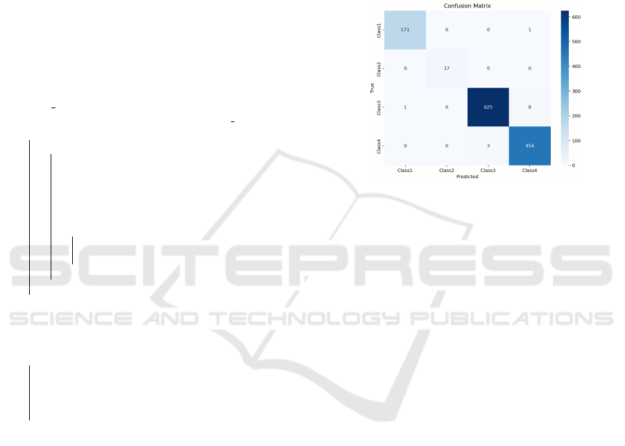
Figure 3 shows Class 1 (Very mild dementia) is
mostly accurate, with some misclassification as Class
4 (Non-dementia) due to feature overlap. Class 2
(Mild dementia) performs well despite a smaller sam-
ple size, with minimal misclassifications. Class 3
(Moderate dementia) achieves the highest accuracy,
with minor misclassification into Class 4. Class 4 also
performs strongly, with slight misclassification into
Class 3, potentially due to shared features or limited
training diversity. Overall classification efficiency is
98.75%.
Figure 2: Confusion matrix illustrating the classification
performance of the ResNet50-based hybrid CNN model.
Misclassifications occur where images predicted
as Class 2 belong to Classes 1 or 3 (see Figure 4),
indicating overlapping features. Class 3 predictions
are generally accurate but still prone to confusion due
to shared characteristics with other classes. Similarly,
Class 1 is occasionally misclassified as Class 2, high-
lighting challenges in distinguishing subtle patterns
between these classes.
Figure 5 (4) illustrates the loss function during
training. Initially (0–500 steps), a rapid decrease indi-
cates effective learning and weight adjustments. Sub-
sequently, the loss stabilizes, suggesting convergence.
The stable curve, without oscillations, indicates min-
imal risk of overfitting.
Figure 6 (5) shows the training loss trajectory.
Initially, a steep decline reflects rapid parameter ad-
justments to capture dominant patterns. Later, the
curve flattens asymptotically, indicating the model’s
approach to optimal capacity. The absence of fluctua-
tions suggests a stable training process with appropri-
ate learning rates and model stability.
Figure 7 (6) depicts the Train Loss function over
training steps. Initially, a sharp increase suggests a
high learning rate or complex parameter adjustments.
After step 1500, the loss stabilizes, indicating equilib-
rium in the optimization process.
Figure 8 (7) shows the training loss sharply de-
clining during the first 500 steps, reflecting efficient
learning. Between steps 500 and 1500, the decrease
slows, and the curve levels off near step 1500, indi-
Leveraging Deep Q-Network Agents with Dynamic Routing Mechanisms in Convolutional Neural Networks for Enhanced and Reliable
Classification of Alzheimer’s Disease from MRI Scans
1177

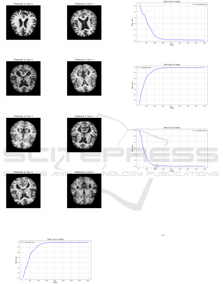
(a) Predicted: 2, True: 2. (b) Predicted: 3, True: 3.
(c) Predicted: 2, True: 2. (d) Predicted: 3, True: 3.
(e) Predicted: 3, True: 3. (f) Predicted: 3, True: 3.
(g) Predicted: 2, True: 0. (h) Predicted: 3, True: 3.
Figure 3: Classification results for selected first 8 cases
from MRI images using a hybrid CNN model.
Figure 4: F1 metrics progression of the F1 score during
training.
cating convergence. The loss stabilizes close to zero,
demonstrating effective error minimization.
Figure 5: Validation Loss progression of validation loss
across training epochs.
Figure 6: Validation Precision progression of validation
precision across training epochs.
Figure 7: Classification training loss per step.
The classification model was evaluated using a
loss function on training and validation data, with
the elbow method determining the optimal stopping
point. Key metrics such as Precision, Recall, and F1-
Score were used for assessment (31). Cross-entropy
was employed as the loss function for multiclass clas-
sification (29).
L(y, ˆy) = −
1
N
N
∑
i=1
C
∑
c=1
y
i,c
log(
ˆ
i, c) (29)
The Training and Validation Loss graphs show
a rapid decline at the start, indicating quick pattern
recognition. Between 3000-4000 steps, the decline
slows, marking the elbow point. The first difference
in the loss function, representing the rate of change,
is calculated (30).
∆L(t) = L(t) −L(t −1) (30)
The elbow point occurs when the change ∆L(t) is
below the established threshold ε (31).
∆L(t) < ε (31)
ICAART 2025 - 17th International Conference on Agents and Artificial Intelligence
1178

Figure analysis shows ∆L(t) stabilizing after
3,000 steps, suggesting training can stop to minimize
overtraining and optimize generalization. Using the
elbow method, training stops at t
∗
when the average
loss change over the last k steps is below ε (32).
1
k
k−1
∑
j=0
|∆L(t − j)| < ε (32)
Loss charts and evaluation metrics indicate that ε
is reached around 3000-4000 steps, suggesting min-
imal gains from further training. Using the elbow
method and metrics like Precision, Recall, and F1-
Score, the optimal stopping point was identified, en-
suring sufficient accuracy and stability.
4.1 Adaptivity of Intelligent Routing
Algorithm
Training consists of 30 episodes, each with 2,000
steps, where input data is randomly assigned, and
routing paths are refined using rewards based on con-
nection quality.
Routing performance is tested in 50 experiments
across 4 scenarios, each lasting 2,000 steps with ran-
dom topologies. Results are averaged to evaluate
routing and classification performance.
5 CONCLUSIONS AND FUTURE
WORK
The proposed model achieved 98.75% accuracy in
Alzheimer’s classification. Future work will focus on
incorporating attention mechanisms and testing on di-
verse datasets to improve generalization and robust-
ness.
REFERENCES
Abhishek, K., Jain, A., and Hamarneh, G. (2024).
Investigating the quality of dermamnist and fitz-
patrick17k dermatological image datasets. arXiv
preprint arXiv:2401.14497.
Afshar, P., Heidarian, S., Naderkhani, F., Oikonomou,
A., Plataniotis, K. N., and Mohammadi, A. (2020).
Covid-caps: A capsule network-based framework for
identification of covid-19 cases from x-ray images.
Pattern Recognition Letters.
Afshar, P., Mohammadi, A., and Plataniotis, K. N. (2018).
Brain tumor type classification via capsule networks.
In 2018 25th IEEE International Conference on Image
Processing (ICIP).
Bai, J., Sun, J., Wang, Z., Zhao, X., Wen, A., Zhang, C.,
and Zhang, J. (2024). An adaptive intelligent rout-
ing algorithm based on deep reinforcement learning.
Computer Communications, 216:195–208.
Bengio, E., Bacon, P.-L., Pineau, J., and Precup, D. (2015).
Conditional computation in neural networks for faster
models. arXiv preprint arXiv:1511.06297.
Bushara, A. R., Kumar, R. V., and Kumar, S. S. (2024).
Classification of benign and malignancy in lung can-
cer using capsule networks with dynamic routing al-
gorithm on computed tomography images. Journal of
Artificial Intelligence and Technology, 4(1):40–48.
He, K., Gkioxari, G., Doll
´
ar, P., and Girshick, R. (2017).
Mask r-cnn. In Proceedings of the IEEE International
Conference on Computer Vision, pages 2961–2969.
Jia, X., Li, J., Zhao, B., Guo, Y., and Huang, Y. (2022). Res-
capsnet: Residual capsule network for data classifica-
tion. Neural Processing Letters, 54(5):4229–4245.
Jiao, Z. and et al. (2019). Dynamic routing capsule net-
works for mild cognitive impairment diagnosis. In
Medical Image Computing and Computer Assisted In-
tervention – MICCAI 2019, volume 11767 of Lecture
Notes in Computer Science, pages 620–628. Springer,
Cham.
Leszek, J. (2012). Choroba alzheimera: obecny stan
wiedzy, perspektywy terapeutyczne. Polski Przeglad
Neurologiczny, 8(3):101–106.
Madhu, G., Govardhan, A., Srinivas, B. S., Sahoo, K. S.,
Jhanjhi, N. Z., Vardhan, K. S., and Rohit, B. (2021).
Imperative dynamic routing between capsules net-
work for malaria classification. CMC-Computers Ma-
terials & Continua, 68(1):903–919.
Pawan, S. J., Sharma, R., Reddy, H., Vani, M., and Rajan,
J. (2023). Widecaps: A wide attention-based capsule
network for image classification. Machine Vision and
Applications, 34(4):52.
Sabour, S., Frosst, N., and Hinton, G. E. (2017). Dynamic
routing between capsules. arXiv:1710.09829.
Sadeghnezhad, E. and Salem, S. (2024). Inceptioncapsule:
Inception-resnet and capsulenet with self-attention
for medical image classification. arXiv preprint
arXiv:2402.02274.
Valadarsky, A., Schapira, M., Shahaf, D., and Tamar, A.
(2017). A machine learning approach to routing.
arXiv preprint arXiv:1708.03074.
Xi, Y., Li, M., Zhou, F., Tang, X., Li, Z., and Tian, J. (2023).
Se-inception-resnet model with focal loss for trans-
mission line fault classification under class imbalance.
IEEE Transactions on Instrumentation and Measure-
ment.
Yadav, S. and Dhage, S. (2024). Te-capsnet: Time effi-
cient capsule network for automatic disease classifi-
cation from medical images. Multimedia Tools and
Applications, 83:49389–49418.
Leveraging Deep Q-Network Agents with Dynamic Routing Mechanisms in Convolutional Neural Networks for Enhanced and Reliable
Classification of Alzheimer’s Disease from MRI Scans
1179