Double Q-Learning for a Simple Parking Problem:

Propositions of Reward Functions and State Representations

Przemysław Kle¸sk

Faculty of Computer Science and Information Technology, West Pomeranian University of Technology in Szczecin,

ul.

Zołnierska 49, 71-210 Szczecin, Poland

Keywords:

Car Parking, Double Q-Learning, Neural Approximations, Parameterized Reward Functions, State

Representations.

Abstract:

We consider a simple parking problem where the goal for the learning agent is to park the car from a range

of initial random positions to a target place with front and back end-points distinguished, without obstacles

in the scene but with an imposed time regime, e.g. 25s. It is a sequential decision problem with a continuous

state space and a high frequency of decisions to be taken. We employ the double Q-learning computational

approach, using the bang–bang control and neural approximations for the Q functions. Our main focus is laid

on the design of rewards and state representations for this problem. We propose a family of parameterized

reward functions that include, in particular, a penalty for the so-called “gutter distance”. We also study several

variants of vector state representations that (apart from observing velocity and direction) relate some key points

on the car with key points in the park place. We show that a suitable combination of the state representation

and rewards can effectively guide the agent towards better trajectories. Thereby, the learning procedure can be

carried out within a reasonably small number of episodes, resulting in high success rate at the testing stage.

1 INTRODUCTION

Driving a car can be seen as a sequential decision

problem that can be subjected to reinforcement learn-

ing (RL) algorithms, Q-learning in particular. Deci-

sions in such a task are commonly called “microde-

cisions” because of their high frequency

. Human

drivers also take many small decisions in order to:

correct velocity or direction, glance in the mirror, start

to brake, react to other vehicles movement, etc. Some

of those are half-conscious or reﬂexive decisions (Sall

et al., 2019; Sprenger, 2022).

In this paper we consider a simpliﬁed variant of

the car parking problem, where the goal for the learn-

ing agent is to drive the car from an initial position

(drawn from a certain random distribution) to the tar-

get park place with front and back end-points distin-

guished, and to fully stop the car there. No obstacles

are present in the scene but the task must be com-

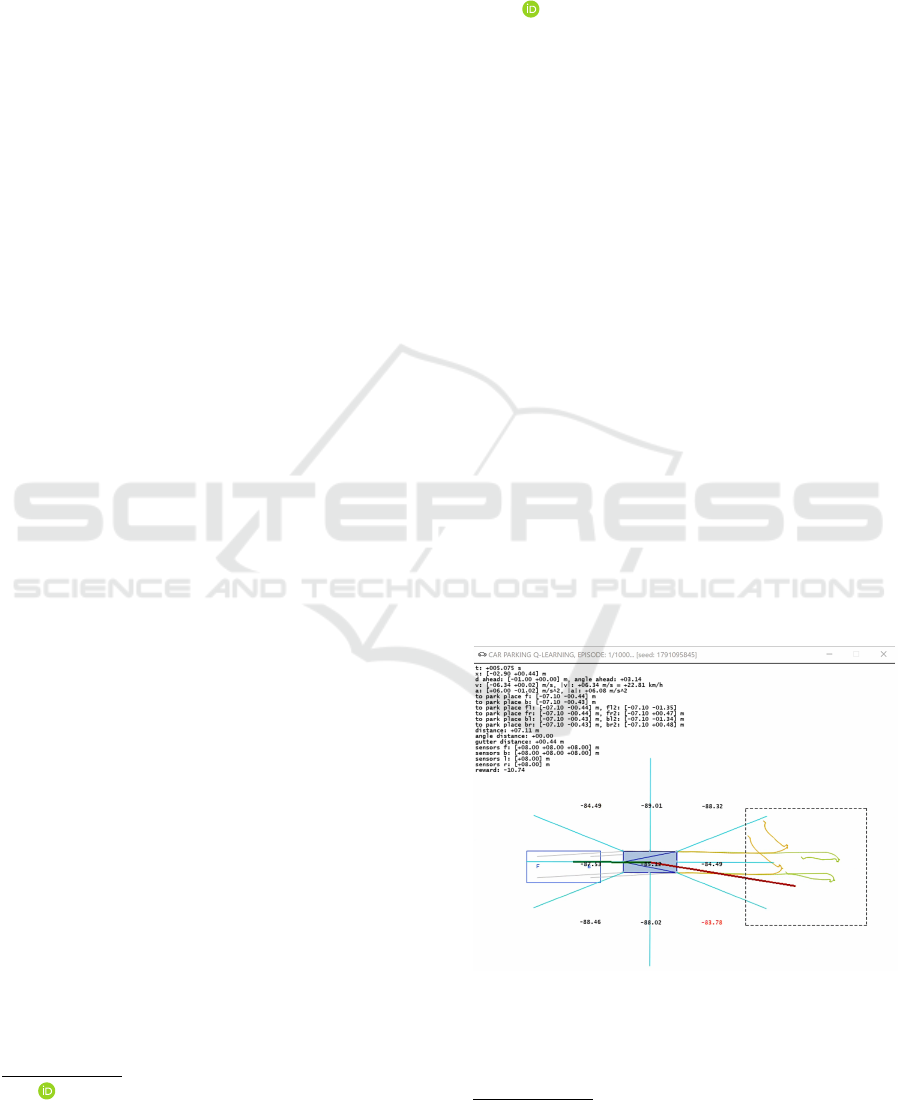
pleted within an imposed time limit, e.g. 25 s. Fig. 1

provides an example illustration of this problem set-

ting — the non-ﬁlled light blue rectangle represents

https://orcid.org/0000-0002-5579-187X

Despite the name, gaps between decision moments are

not necessarily at the level of microseconds.

the park place (with ‘F’ and ‘B’ letters denoting its

front and back) and the dashed border marks the re-

gion of random initial positions for the car

Figure 1: Example illustration of the simple car parking

problem.

We implement the bang–bang control scenario in

this paper. This means that there exists a ﬁnite set

The car’s initial direction angle is also drawn from a

certain random range.

156

KlÈl’sk, P.

Double Q-Learning for a Simple Parking Problem: Propositions of Reward Functions and State Representations.

DOI: 10.5220/0013302100003890

Paper published under CC license (CC BY-NC-ND 4.0)

In Proceedings of the 17th International Conference on Agents and Artiﬁcial Intelligence (ICAART 2025) - Volume 1, pages 156-171

ISBN: 978-989-758-737-5; ISSN: 2184-433X

of acceleration vectors (or equivalently force vectors)

that can be applied on the car at decision moments.

An applied acceleration can be either completely on

or off. Fractional application is not permitted. In

Fig. 1, the dark green line is the current velocity vec-

tor — the car is traveling roughly forwards (to the left

of the image); whereas the red line, directed almost

oppositely, represents the imposed acceleration vec-

tor — the car starts to brake and gently turn left as it

is approaching the park place. Light orange and green

curves mark traces of front and back wheels, respec-

tively. Gray lines represent vectors pointing from the

car corners to their ideal positions in the park place.

The general computational approach that we have

employed in the reasearch underlying this paper

is compliant with the double Q-learning technique

(Hasselt, 2010; Hasselt et al., 2016). This means there

are two approximators of the Q function involved.

We use several-layers-deep, dense neural networks

with ReLU activations as approximators. One net-

work is used for making decisions during the parking

attempts, and simultaneously for learning via expe-

rience replay. Weights of that network are updated

quite frequently. The second network, with the same

structure, stays frozen for long periods and plays the

role of a “pseudo-oracle”. It serves the purpose of

providing stable target values for the supervised learn-

ing of the ﬁrst network. After suitably many training

steps, the target network gets switched — that is, the

weights from the online network are copied to the tar-

get network.

1.1 A “Needle in a Haystack”

Motivation

The main points of interest in this paper are reward

functions and state representations for the deﬁned

parking problem. It should be well understood that in

rich environments with continuous state spaces, sim-

ple non-informed reward functions do not work well.

Imagine a car parking agent that starts wandering ran-

domly 10 meters away from the park place. If, for

example, that agent is rewarded solely with a −∆t

value after each small time step in which he did not

succeed to “land” in the park place (e.g. −0.1 s re-

ward for the time consumed per step), then clearly he

should not be expected to learn anything. The func-

tion being approximated is ﬂat almost everywhere.

The fact that the success event requires the car to be

accurately placed (with only a small deviation toler-

ated distance- and angle-wise), and moreover fully

stopped, makes such an event extremely unlikely to

be discovered accidentally — just like a “needle in a

haystack”. Naturally, one might try to extend the −∆t

reward with an extra summand that estimates the re-

maining time needed to reach the target. This could

be done e.g. based on the remaining straight-line dis-

tance and assuming some average velocity while ma-

neuvering. As we show in the paper, such an exten-

sion is only a minor improvement, not sufﬁcient to

signiﬁcantly speed up the learning process.

1.2 Main Contribution

In the paper we propose and study a parameterized

reward function for the parking problem, with three

penalty terms pertaining to: (a) the straight-line dis-

tance, (b) the angular deviation between direction

vectors of the car and the park place, and (c) an ad-

ditional quantity named the “gutter distance”. We

indicate good proportions between those terms, rep-

resented by suitable penalty coefﬁcients discovered in

experiments.

Furthermore, we experiment with several vari-

ants of state representations with information re-

dundancy that constitute the input to neural models.

Apart from the car direction and velocity, the rep-

resentations include additional vector-based informa-

tion that relates key points on the car with key points

in the park place. Our results demonstrate that a suit-

able combination of the state representation and re-

wards can effectively guide the parking agent towards

better trajectories. Thereby, the learning quality is im-

proved and the process can be carried out within a

reasonably small number of episodes.

2 PRELIMINARIES

2.1 Q Functions

Given a policy P — a mapping from the set of states

to the set of actions, the Q

(s,a) function is de-

ﬁned to return the expected sum of all future rewards

t+1

t+2

,.. . (random variables), discounted expo-

nentially by a decay rate γ ∈ [0,1), conditional on the

fact that at the starting state S

= s one performs action

a, and from thereafter follows the policy P :

(s,a)=E



t+1

+γR

t+2

+γ

t+3

+···|S

=s,A

=a;P



(1)

This means that for all attained subsequent states s

t+k

k = 1,2,. .. , the agent takes actions a

t+k

yielded by

the policy: a

t+k

= P (s

t+k

), whereas the initial action

Capital letters under the expectation E(·) in (1) repre-

sent random variables and lowercase ones their realizations

i.e. the values attained.

Double Q-Learning for a Simple Parking Problem: Propositions of Reward Functions and State Representations

157

a can be arbitrary, not necessarily compliant with the

policy.

In environments with stochastic transitions and re-

wards, an action a performed by the agent in a state

s can result in various pairs (r,s

′

) of the reward value

and the next state; sometimes differing only slightly.

In such a case, the recursive deﬁnition of the optimal

action value Q

∗

(s,a), known as the Bellman optimal-

ity equation, takes into account the probabilities (or

densities) of transitions, and is:

∗

(s,a) =

∑

′

P(r,s

′

|s,a)



r + γ max

′

∗

′

)



, or

(2)

∗

(s,a) =

r,s

′

p(r,s

′

|s,a)



r + γ max

′

∗

′

)



dr ds

′

(3)

In deterministic environments, a ﬁxed (s,a) pair al-

ways produces a speciﬁc next pair of (r,s

′

), and the

Bellman equation reduces to:

∗

(s,a) = r(s

′

) + γmax

′

∗

′

), (4)

where for our purposes we choose to write r(s

′

), un-

derstood as r(s

′

) ≡ r(s,a), to represent the fact that

our deterministic rewards shall be implied by the

reached state s

′

alone.

2.2 Double Q-Learning

In contrast to small grid environments, where Q val-

ues can be updated in lookup tables inductively with-

out special risks, reinforcement learning for larger

problems, based on Q function approximation, re-

quires caution due to potential violations of the ele-

mentary i.i.d. principle of machine learning. It states

that data examples ought to be independent and iden-

tically distributed. There are three elements that may

contribute to the violation of i.i.d.

Firstly, consecutive states along a certain trajec-

tory are obviously not independent, but highly cor-

related. An approach that diminishes this problem

is experience replay (Mnih et al., 2013; Mnih et al.,

2015; Hasselt et al., 2016). It collects the experience

quadruplets — state, action, reward, next state — into

a large buffer, and from time to time triggers the train-

ing based on a random data subsample drawn from

this buffer independently and with repetitions (a boot-

strap batch). This effectively decorelates the data.

Secondly, suppose that

Q(s,a;

w) denotes our

working model parameterized by weights

w. With

this model we would like to approximate Q

∗

(s,a) for

all (s,a), i.e. to have

Q(s,a;

w) ≈ Q

∗

(s,a). Suppose

also that (s

′

) is a single i-th experience drawn

from our buffer. To train

Q using this experience, one

needs to prepare a certain target value y

∗

for the input

pair (s

), so that the supervised regression task can

be performed. Mathematically, such a target value is

implied by the right-hand-side of Bellman equation

(4) — the ideal target value. Therefore, it may seem

the task is to minimize the following squared error



Q(s

;

w) − (r

+ γ max

′

∗

′

)

| {z }

∗

)



(5)

with respect to

w. Doing so, e.g. by means of the

stochastic gradient descent, would mean to update

weights e.g. as follows:

w :=

w − η



Q(s

;

w) − (r

+γmax

′

∗

′

))



· ∇

Q(s

;

w), (6)

where η ∈ (0,1] stands for a learning rate constant

and ∇

Q(·) for the gradient of our approximator. Yet,

in practice it is impossible to prepare the target y

∗

shown in (5), because true oracles Q

∗

do not exist and

we simply do not know the value of Q

∗

′

). . . One

could be tempted to set y

∗

:= r

+ γmax

′

Q(s

′

;

instead. But that would mean that the target values

one tries to approximate with model

Q are themselves

computed using

Q. This phenomenon, known as a

“pursuit of non-stationary target”, may lead to an un-

stable learning process.

The idea behind double Q-learning solves this

problem by introducing the second model, say

Q(·;

w), that can be regarded as a pseudo-oracle serv-

ing the purpose of providing a stable second summand

for the target values as follows (Hasselt, 2010; Hasselt

et al., 2016; Mnih et al., 2013):

∗

:= r

+ γ max

′

Q(s

′

;

w). (7)

For neural networks applied as approximators, the

Q model is often referred to as the ‘target network’,

while the main operating model

Q as the ‘online net-

work’.

Two approaches for updating

Q are met in prac-

tice. In the ﬁrst one,

Q stays frozen for a long period

(so that many training steps of

Q can take place us-

ing stable targets) and then

Q gets replaced by mak-

ing a hard switch of weights:

w :=

w. In the second

approach,

Q is updated slowly, but continuously, to-

wards

Q via a moving average, e.g:

w := 0.999

w +

0.001

w. This way or another, the idea with two mod-

els stabilizes signiﬁcantly the learning process (Fujita

et al., 2021; Kobayashi and Ilboudo, 2021).

ICAART 2025 - 17th International Conference on Agents and Artiﬁcial Intelligence

158

The third element that endangers the i.i.d. is more

subtle. It pertains to the max operator present in (7),

which under the stochastic setting is biased towards

overestimations of future rewards. Both mathematical

and empirical evidence support this claim (Thrun and

Schwartz, 1993; Hasselt, 2010; Hasselt et al., 2016;

Sutton and Barto, 2018). The following simple, yet

elegant, trick circumvents the problem. Noting that

(7) can be equivalently rewritten as

∗

:= r

+ γ



′

, argmax

′

Q(s

′

;

w);



, (8)

one prefers instead to use the following estimation of

the target value:

∗

:= r

+ γ



′

, argmax

′

Q(s

′

;

w);



. (9)

It means the online model

Q is still used to pick

the ‘best’ next action, but the value of that action

is estimated with the target model

Q. An apt anal-

ogy to it is a situation where two measurement in-

struments (e.g. scales for measuring weights in kilo-

grams), each biased with a certain stochastic error, are

used to discover a maximum value over a certain col-

lection of objects. Using one instrument to indicate

the ‘argmax’ and the other to indicate the value for

this argument is a practical protection against the sta-

tistical overestimation.

3 RELEVANT WORK

First of all, it should be clearly remarked that our di-

rect research interests are not located in the domain

of AGVs (autonomous ground vehicles) but in rein-

forcement learning itself. We focus on the design of

reward functions in RL problems, where an immedi-

ate reward signal is not present or is extremely sparse

(“needle in a haystack”). Therefore, the simple park-

ing problem should be treated as a toy example serv-

ing that purpose in this research. Readers directly in-

terested in recent advances in the realm of AGVs and

APSs (automatic parking systems) can be addressed

e.g. to two works (Zeng et al., 2019; Cai et al., 2022)

that employ geometric methods and control theory,

or to (Chai et al., 2022; Li et al., 2018) where neu-

ral networks are applied to approximate near-optimal

trajectories; the latter involves also RRTs (Rapidly-

exploring Random Trees).

As regards the general topic of rewards in RL

(without connection to the parking problem), worth

attention is a recent paper due to Sowerby, Zhou and

Littman (Sowerby et al., 2022). It discusses how

reward-design choices impact the learning process

and tries to identify principles of good reward design

that quickly induce target behaviors. Moreover, us-

ing concepts of action gap and subjective discount,

the authors propose a linear programming technique

to ﬁnd optimal rewards for tabular environments.

As regards works with similarity to ours and per-

taining to both contexts — rewards and RL-based

parking — the following two can be pointed: (Aditya

et al., 2023; Zhang et al., 2019). In (Aditya et al.,

2023), Aditya et al. also employ the double Q-

learning. Their simulated parking lot contains ob-

stacles (other cars parked), but it has a ﬁxed lay-

out and a predeﬁned loop path along which the car

cruises before it ﬁnds a free spot. Only then, the ac-

tual RL-based parking maneuvers begin. The reward

function from (Aditya et al., 2023) involves distance

and angle deviation and decays exponentially as those

quantities increase. The authors report 95% success

rate after 24 hours of training (Intel Core i5-1135G7

CPU, IRIS Xe GPU). Unfortunately, no details on

the neural network structure are provided. In (Zhang

et al., 2019), Zhang et al. apply the policy gradient

approach using a two-layer deep network with 100

and 200 ReLU-activated neurons, respectively. Their

hand-crafted reward function contains four pieces of

information: closeness to the slot center, ‘parallelism’

of car and park main axes, penalties for line-pressing

and side deviations. Experiments include scenes with

◦

, 45

◦

and 30

◦

initial angles between the car and the

parkplace. The reported results focus on ﬁnal devia-

tions from the wanted goal position which range from

about 0.37m to 0.48 m sideways and are up to ≈ 1m

lengthwise.

Obviously, due to different environment settings

and the problem itself, it is impossible to fairly

compare our results against the ones from (Aditya

et al., 2023; Zhang et al., 2019). On one hand,

the lack of obstacles is a clear simpliﬁcation in our

problem variant; on the other, we take into account a

demanding time limit and a broader range of initial

angles and positions (some of them remote) —

hence, an environment that requires more exploration

from the RL perspective and more capable models

to suitably approximate Q values over a richer state

space. We remind that in (Aditya et al., 2023; Zhang

et al., 2019) the actual parking maneuvers start in

the close proximity of the goal. Yet, if despite all

differences the raw numbers were to be compared,

then we can report obtaining 7 models with success

rates exceeding 95% (two of them reaching 99%)

having the ﬁnal deviations of at most 41 cm for both

axes. Each model was trained for only 10 k episodes

and ≈5 h (all details in Section 7).

Double Q-Learning for a Simple Parking Problem: Propositions of Reward Functions and State Representations

159

We believe an important distinction of our re-

search is that we do not work with a single reward

function with ﬁxed coefﬁcients as it was the case in

(Aditya et al., 2023; Zhang et al., 2019) (a dogmatic

approach). Instead, we work with a parameterized

family of reward functions and discover good propor-

tions between the involved quantities over multiple

experiments.

4 NOTATION, SETTINGS,

PHYSICS

We start this section by providing the link to the

repository of the project associated with this paper:

https://github.com/pklesk/qlparking. It provides access

to source codes, logs for selected models and videos

with parking maneuvers. The implementation has

been done in the Python programming language. All

settings pertaining to physics and car behavior are de-

ﬁned in the script ./src/defs.py.

Our car model for simulations is of length l =

4.405m and width w = 1.818 m. µ

= 0.6 and µ

0.3 denote its coefﬁcients of static and kinetic fric-

tion, respectively. We do not specify the car’s mass,

since we are going to operate only on accelerations

rather than forces (masses not needed). The gravita-

tional acceleration constant is denoted by g and for

computations equal to 9.80665m/s

The complete information about the car’s position

and orientation is deﬁned by its current center point

⃗x and a unit direction vector

⃗

d (ahead direction at

which the car is looking). Additionally, where use-

ful, we write

⃗

to denote the unit vector pointing to

the right of the car.

⃗

d becomes

⃗

after 90

◦

clockwise

rotation. The car’s velocity vector is denoted by ⃗v.

All of the above are planar vectors (with two Carte-

sian coordinates), which means the surface of simu-

lated scenes is treated as ﬂat. Where mathematically

needed, the notation additionally includes a time sub-

script e.g. ⃗x

⃗

,⃗v

, or is overloaded to writings such

as ⃗x

⃗

,⃗v

, to be read as ‘in state s’, if we need to

explicitly emphasize the dependence on a state.

As regards the park place, it is of length l

6.10m and width w

= 2.74 m, with position and ori-

entation described, analogically, by vectors ⃗x

⃗

p,R

, remaining constant in time (the park place does

not move). Therefore, the ideal position for the car

to be parked at is described by the following corner

points:

⃗x

p,FL

=⃗x

+ 0.5 l

⃗

− 0.5 w

⃗

p,R

, (front-left)

⃗x

p,FR

=⃗x

+ 0.5 l

⃗

+ 0.5 w

⃗

p,R

, (front-right)

⃗x

p,BL

=⃗x

− 0.5 l

⃗

− 0.5 w

⃗

p,R

, (back-left)

⃗x

p,BR

=⃗x

− 0.5 l

⃗

+ 0.5 w

⃗

p,R

. (back-right).

In accordance with the bang–bang control sce-

nario, we deﬁne the set of three magnitudes for the

forward-backward accelerations:



−1,·

=−7.0m/s

0,·

=0.0m/s

+1,·

=+8.0m/s



(10)

and three magnitudes for the side accelerations (turn-

ing):



·,−1

=−1.0m/s

·,0

=0.0m/s

·,+1

=+1.0m/s



(11)

Therefore, the following set of 9 possible actions

becomes generated via the Cartesian product of the

above two sets:

A =

⃗a

j,k

= a

j,·

⃗

d + a

·,k

⃗

( j, k) ∈ {−1,0,1}×{−1, 0,1}

. (12)

More simply, the set of actions can be treated equiva-

lently to 9 symbolic directions {↙,↓, ↘,←, ◦,→,↖

,↑,↗}, meaning: ‘backwards left’, ‘backwards’, . . . ,

‘forwards right’, with the empty action ‘◦’ represent-

ing no acceleration applied.

The time step chosen for simulations was

δt=25 ms. Algorithm 1 presents the basic computa-

tions that take place when the time moment becomes

switched from t to t + δt, performed to update the

car’s velocity, position and direction, based on the ap-

plied acceleration vector ⃗a

∈A with static and kinetic

friction taken into account.

The chosen δt = 25 ms means that 40 ‘microde-

cisions’ per second could potentially be taken by the

agent. Such a granularity seems a bit too ﬁne for the

parking task. One reason is that the imposed acceler-

ations would change very fast and unrealistically un-

der the bang–bang control. The second is that human

drivers do not take decisions so frequently. There-

fore, to make the agent more human-like, the time

gap between steering steps was deﬁned as ∆t = 4 δt =

100ms. This implies ten decisions per second taken

by the agent.

To avoid modelling static frictions directed sideways,

a simple condition prevents the vehicle from making in-

stantaneous turns at low velocities (so that it does not

behave like a military tank): if ∥v

∥ < 0.75 m/s (see

defs.CAR_MIN_VELOCITY_TO_TURN) then only longitudinal compo-

nents of imposed side components are ignored.

see constants: QL_DT = 0.025 and QL_STEERING_GAP_STEPS = 4

in the ./src/main.py

ICAART 2025 - 17th International Conference on Agents and Artiﬁcial Intelligence

160

if ∥⃗v

∥ = 0.0 and ∥⃗a

∥ > 0.0 then

:= min{µ

g/∥⃗a

∥,1.0};

⃗a

:= (1.0 − α

)⃗a

;

end

:= 0.0;

if ∥⃗v

∥ > 0.0 then

∥ ¯v∥ := ∥⃗v

+ 0.5⃗a

δt∥;

:= min{µ

gδt/∥¯v∥,1.0};

end

⃗x

t+δt

:=⃗x

+ (1.0 − α

)(⃗v

δt + 0.5⃗a

δt

);

⃗v

t+δt

:= (1.0 − α

)(⃗v

+⃗a

δt);

if ∥⃗v

t+δt

∥ > 0.0 then

⃗

t+δt

:= sgn



⟨⃗v

t+δt

⃗

⟩



⃗v

t+δt

/∥⃗v

t+δt

∥;

end

Algorithm 1: Single step of simulation (updates of car

physics.

5 PARAMETERIZED REWARD

FUNCTION

As stated in the motivation, our goal is to propose

such a reward function that shall guide the agent to-

wards better trajectories more quickly while perform-

ing the Q-learning. Apart from −∆t (time consumed

between decision steps) and the remaining distance

∥⃗x −⃗x

∥, two more quantities will be taken into ac-

count. Moreover, we want our ﬁnal function to pre-

serve a consistent physical interpretation of the “neg-

ative time”, and thus be expressible, e.g., in seconds.

First, we deﬁne the angular deviation φ(

⃗

d) be-

tween direction vectors of the car and the park place,

based on their inner product:

φ(

⃗

d) = arccos⟨

⃗

⟩ ∈[0,π]. (13)

⃗

, being a constant, is not speciﬁed as an explicit

argument of φ.

The car is considered successfully parked if the

following conditions are met:

∥⃗x −⃗x

∥ ⩽ 0.15 w

and φ(

⃗

d) ⩽ π/16 and ∥⃗v∥ = 0.0.

(14)

The tolerance constants

present in (14) imply that the

car’s center can deviate from the park place center by

at most 15% of the place width (≈41 cm) and also that

the angle between the car’s direction and the optimal

direction can deviate by at most 11.25

◦

We are now going to deﬁne a quantity named the

“gutter distance”. It represents the distance between

the car’s center point and its projection onto the axis

defs.CONST_PARKED_MAX_RELATIVE_DISTANCE_DEVIATION = 0.15

defs.CONST_PARKED_MAX_ANGLE_DEVIATION = np.pi / 16

deﬁned by the park place

, and can be computed as:

g(⃗x) =



9 ⟨

⃗

p,R

,⃗x

⟩+⟨

⃗

p,R

,⃗x ⟩





∥

⃗

p,R

∥



⟨

⃗

p,R

,⃗x−⃗x

⟩



. (15)

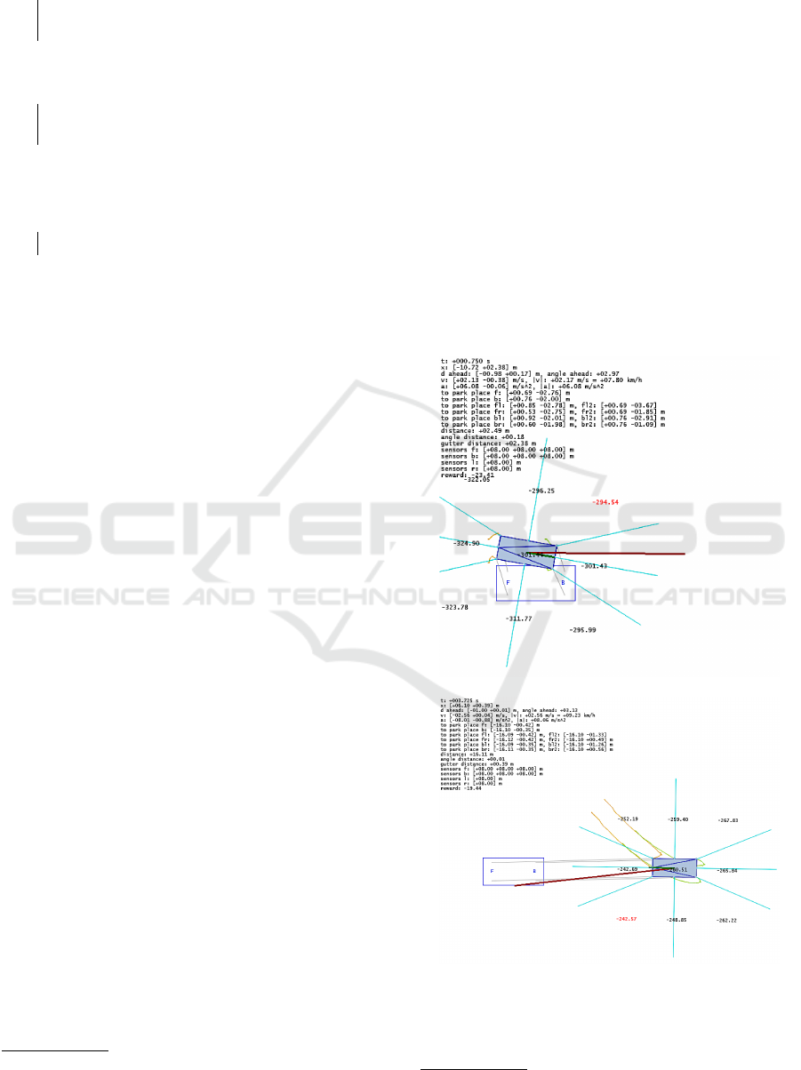
Intuitively, the presence of this quantity in the re-

ward should help the learning agent distinguish better

between less and more promising states as regards the

future trajectory needed to complete the task. For ex-

ample, states where the car is quite far from the park

place but approximately on the right track to approach

the target (small “gutter distance”) are more promis-

ing (Fig. 2b) than states where the car is near the park

place but deviated sideways (Fig. 2a). In the latter

case, more maneuvering needs to be invested to com-

plete the task (note distances and

Q values reported in

the ﬁgure).

(a) dist. ≈2.49 m, gutter dist. ≈2.38 m, max

Q(s,a;

w)≈ −294.54

(b) dist. ≈16.11 m, gutter dist. ≈0.39 m, max

Q(s,a;

w)≈ −242.57

Figure 2: Comparison of two states: (a) with small straight-

line distance but future trajectory demanding, (b) with large

straight-line distance but future trajectory easy (small gutter

distance).

the axis passing through points F (front) and B (back)

Double Q-Learning for a Simple Parking Problem: Propositions of Reward Functions and State Representations

161

Finally, we propose the following parameterized

function that rewards the agent for being in state s

′

(after taking action a in s):

r(s

′











0; if car successfully parked in s

′



∆t+λ

∥⃗x

′

−⃗x

∥

{z }

distance

+λ

φ(

⃗

′

)/π

| {z }

normed

angular deviation

+λ

g(⃗x

′

)

|{z}

gutter distance



;

(16)

where parameters λ

,λ

⩾ 0 are penalty coefﬁ-

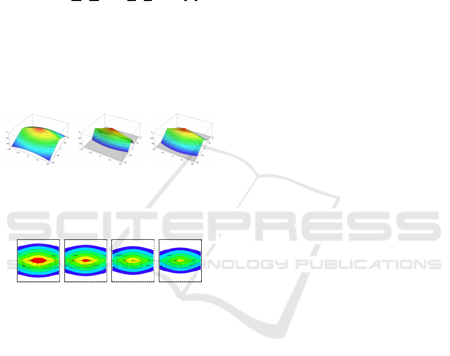
cients. Figures 3, 4 show example plots of (16) when

⃗x

=(0.0,0.0),

⃗

=(−1.0,0.0).

(λ

,λ

) (λ

,λ

) (λ

,λ

)

= (1.0,1.0, 1.0) = (1.0,2.0, 4.0) = (1.0,4.0, 2.0)

φ = π/8 φ = π/8 φ = π/8

Figure 3: Shapes of reward function (16) for different

penalty coefﬁcients λ

,λ

and a ﬁxed angle φ = π/8 .

= 1.0,λ

= 16.0,λ

= 2.0

φ = 0/4π φ = 1/4π φ = 2/4π φ = 3/4π

41.5

33.2

16.6

-20 -10 0 10 20

-20

-10

41.5

33.2

-16.6

-20 -10 0 10 20

-20

-10

41.5

24.9

-20 -10 0 10 20

-20

-10

41.5

24.9

-20 -10 0 10 20

-20

-10

Figure 4: Contours of reward function (16) for different

angles φ and penalty coefﬁcients ﬁxed to λ

= 1.0, λ

16.0,λ

= 2.0.

One should note that −∆t summand, rather than

−δt, takes part in (16). This means that for s

= s,

the actual reward is collected in state s

′

t+∆t

t+4δt

i.e., at the next decision moment, and the intermediate

physical states s

t+δt

, s

t+2δt

, s

t+3δt

are not rewarded.

Though a meaningful interpretation of reward is

not a must in many RL applications, we note that

(16) is interpretable and expressible in time units.

If e.g. λ

= 2.0 then the second summand rewritten

equivalently to ∥⃗x

′

−⃗x

∥



(1/λ

) can be seen as the

ratio: distance / velocity, and interpreted as estimated

future time needed to cover the remaining distance

when traveling on average at velocity 1/λ

= 0.5 m/s

while maneuvering. Similarly, the reciprocal 1/λ

can be understood as average velocity at which the

agent is able to correct one unit of the gutter distance.

The smaller that velocity is, the higher the importance

of the gutter summand. Deviation φ is a unitless real

number, hence 1/λ

can be seen as an angular veloc-

ity expressed in 1/s units. We decided to norm this

quantity to [0,1] interval (division by π). Thus, the λ

itself can be also interpreted as the time required to

correct the maximum possible deviation of 180

◦

6 STATE REPRESENTATIONS

In this section we propose 13 variants of state repre-

sentations for the considered parking problem. The

representations are feature vectors that constitute in-

puts to neural models

Q and

Q. The nature and in-

formativeness of inputs obviously have a strong im-

pact on the quality of approximations. Yet, without

an experiment it is usually not clear whether particu-

lar pieces of information facilitate or hinder the task.

We take under consideration both the

globally-oriented features that capture a bird’s-eye

view of the environment, and locally-oriented fea-

tures computed relative to the agent. A minimalistic

representation could include: the car’s heading angle

ψ (computed with respect to the global coordinate

system by means of arctan2 function), the signed

magnitude of velocity along that angle, and vectors

⃗

f ,

⃗

b pointing from the car’s front and back central

points, respecitvely, to their counterparts in the park

place (relative features):

⃗

f =⃗x

+ 0.5l

⃗

−



⃗x + 0.5l

⃗



⃗

b =⃗x

− 0.5l

⃗

−



⃗x − 0.5l

⃗



Therfore, the minimalistic representation of a state s

can be:

(ψ,±∥⃗v∥,

⃗

f ,

⃗

. (17)

The above compact notation should be understood

as a concatenation of two scalars and two vectors,

thereby yielding a total of 6 real-numbered features.

An equivalent representation but expressed only in

terms of vectors could be:

(

⃗

d,⃗v,

⃗

f ,

⃗

. (18)

It has 8 features with some redundancy, since

⃗

d =

±⃗v/∥⃗v∥.

Instead of

⃗

f ,

⃗

b, one can introduce four vectors

spanning between the corner points of the car and

their ideal target positions (also with redundancy),

namely:

⃗

=⃗x

p,FL

−⃗x−0.5(l

⃗

d−w

⃗

=⃗x

p,FR

−⃗x−0.5(l

⃗

d+w

⃗

=⃗x

p,BL

−⃗x+0.5(l

⃗

d+w

⃗

=⃗x

p,BR

−⃗x+0.5(l

⃗

d−w

⃗

). (19)

ICAART 2025 - 17th International Conference on Agents and Artiﬁcial Intelligence

162

Alternatively, the following variation is also possible:

⃗

L,2

=⃗x

p,FL

−



⃗x+0.5l

⃗



⃗

R,2

=⃗x

p,FR

−



⃗x+0.5l

⃗



⃗

L,2

=⃗x

p,BL

−



⃗x−0.5l

⃗



⃗

R,2

=⃗x

p,BR

−



⃗x−0.5l

⃗



(20)

where the vectors point to the corners of the target

position but from the central front and central back

points on the car. We refer to them as ‘2nd-type’ cor-

ner vectors. These vectors provide a useful informa-

tion when the car is in the last phase of parking —

covering ﬁnal meters along the right track either for-

wards or backwards. One should realize that in such

cases the angles ∠(

⃗

L,2

⃗

R,2

) and ∠(

⃗

L,2

⃗

R,2

) tend

to π i.e. 180

◦

. Note that it is not the case with the

ﬁrst type of corner vectors. Fig. 5 illustrates different

types of discussed vectors.

Finally, the vector of features may also be ex-

tended with pieces of information that explicitly

take part in the reward function (16), namely:

∥⃗x−⃗x

∥,φ(

⃗

d), g(⃗x). Their presence potentially “re-

lieves” the neural model from computing them indi-

rectly (in intermediate layers). Yet again, such a claim

requires experimental conﬁrmation. Table 1 lists all

representations used in experiments.

Table 1: Variants of state representations.

name

state representation

(pieces of information in state s)

# of

features

avms_fb (ψ, ±∥⃗v∥,

⃗

f ,

⃗

dv_fb (

⃗

d,⃗v,

⃗

f ,

⃗

dv_ﬂfrblbr (

⃗

d,⃗v,

⃗

)

dv_ﬂfrblbr2s (

⃗

d,⃗v,

⃗

)

dv_fb_d (

⃗

d,⃗v,

⃗

f ,

⃗

b,∥⃗x−⃗x

∥)

dv_ﬂfrblbr_d (

⃗

d,⃗v,

⃗

,∥⃗x−⃗x

∥)

dv_ﬂfrblbr2s_d (

⃗

d,⃗v,

⃗

,∥⃗x−⃗x

∥)

dv_fb_da (

⃗

d,⃗v,

⃗

f ,

⃗

b,∥⃗x−⃗x

∥,φ(

⃗

d))

dv_ﬂfrblbr_da (

⃗

d,⃗v,

⃗

,∥⃗x−⃗x

∥,φ(

⃗

d))

dv_ﬂfrblbr2s_da (

⃗

d,⃗v,

⃗

,∥⃗x−⃗x

∥,φ(

⃗

d))

dv_fb_dag (

⃗

d,⃗v,

⃗

f ,

⃗

b,∥⃗x−⃗x

∥,φ(

⃗

d),g(⃗x))

dv_ﬂfrblbr_dag (

⃗

d,⃗v,

⃗

,∥⃗x−⃗x

∥,φ(

⃗

d),g(⃗x))

dv_ﬂfrblbr2s_dag (

⃗

d,⃗v,

⃗

,∥⃗x−⃗x

∥,φ(

⃗

d),g(⃗x))

7 MAIN EXPERIMENTS AND

RESULTS

Experimental Setup. To ensure a fair comparison

of different combinations of reward functions and

state representation, in all experiments we performed

a constant number of 10 k episodes (each with the

time limit of 25s to park the car) and we applied the

same structure for neural models. Training scenes

involved a park place with ﬁxed settings of ⃗x

(−10.0,0.0),

⃗

= (−1.0,0.0) and random initial po-

sitions of the car drawn from uniform distributions:

⃗x ∼ U ([5.0, 15.0] × [−5.0, 5.0]), ψ ∼ U (

π,

π). For

testing, we used 1 k scenes generated by the same dis-

tributions but with different randomization seeds to

verify the generalization ability of obtained models.

Also, for several best models we performed additional

tests where the initial angle was drawn from a broader

distribution: ψ ∼ U(

π,

π), hence a range of 180

◦

instead of 90

◦

. Such tests verify the extrapolative gen-

eralization ability of models.

In each episode we collected experience quadru-

plets (s,a, r,s

′

) separated by time gaps of ∆t = 4δt.

At most 250 experiences could have been collected

per episode. Starting from episode 200 onwards, ﬁt-

ting of the online model

Q was conducted every 20

episodes. In accordance with experience replay, each

ﬁt was based on a bootstrap sample of 65 536 expe-

riences drawn from the buffer, with target values for

regression computed in compliance with formula (9)

using γ = 0.99. A single ﬁt consisted of 1 epoch of

Adam SGD corrections (Kingma and Ba, 2014) using

minibatches of size 128. Starting from episode 1000

onwards, every 500 episodes we were switching the

target network

Q (to become a copy of

Q).

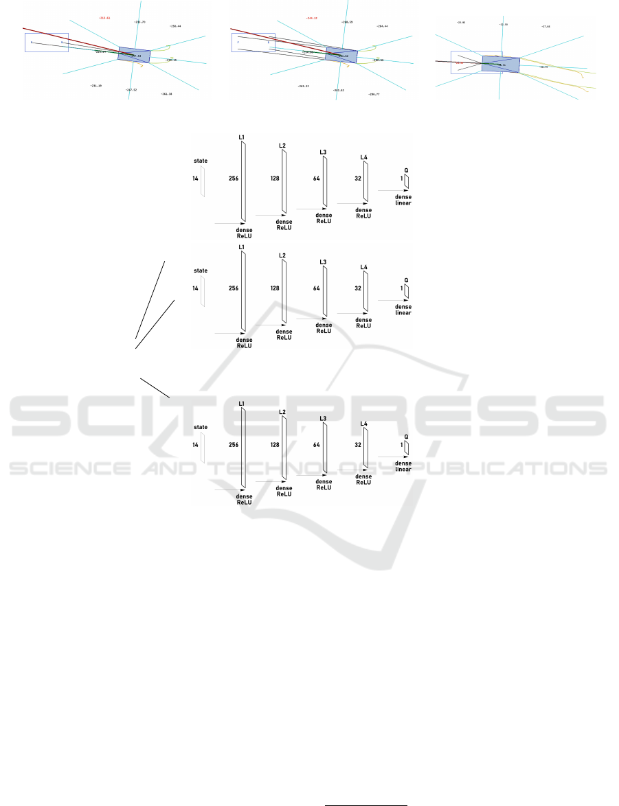
Modular Structure of Neural Models (Approxima-

tors). To remind, a

Q or

Q model takes as its in-

put a vector of features representing a state and re-

turns as the output a vector of predicted (approxi-

mated) action values, one value per each action in

A. Our Python implementation for such models —

class named qapproximations.QMLPRegressor — works

as a wrapper around a collection of standard MLP net-

works

. This means that in our experiments a single

Q (or

Q) model consisted, in fact, of 9 independent

substructures, or equivalently 9 subnetworks, that

did not share weights; see Fig. 6. Each substructure

corresponded to one action in A and was ﬁt based on

experiences related to that action only. Hence, within

calls of ﬁt(X, y, actions_taken) method, the mentioned

bootstrap samples containing 65536 examples were

being partitioned into 9 disjoint subsets (based on the

information from the last argument actions_taken), and

those subsets were still further partitioned into mini-

batches to perform an epoch of Adam algorithm.

We remark that in RL applications this kind of

modular structure for function approximators, some-

times called multi-head structure, is not new (Chen

et al., 2021; Mankowitz et al., 2018; Goyal et al.,

2019), but deﬁnitely less popular than the one with

shared hidden layers and weights (most of DQNs and

DDQNs (Mnih et al., 2013; Mnih et al., 2015; Has-

selt et al., 2016)). However, in our opinion, the popu-

sklearn.neural_network.MLPRegressor (Pedregosa et al., 2011)

Double Q-Learning for a Simple Parking Problem: Propositions of Reward Functions and State Representations

163

(a):

⃗

f ,

⃗

b (b):

⃗

(c):

⃗

Figure 5: Vectors (black segments) between key points on the car and the park place.

INPUT: state representation

7→

Q(s,↙;

7→

Q(s,↓;

7→

Q(s,↗;

OUTPUT: predicted action values

Figure 6: Modular structure of the neural network representing the

Q model with 14 inputs (state representation) and consisting

of 9 independent substructures, one per each action.

lar structure has certain drawbacks related both to the

principles of machine learning and to convergence.

The most important one is the ambiguity on how to

prepare those entries of target vectors that are associ-

ated with non-taken actions. Note that only the taken

action entry is well-deﬁned by the Bellman equation,

e.g. (9).

For the main experiments presented in this sec-

tion, we employed networks in which the mentioned

substructures consisted of 4 hidden dense layers,

each, with the following sizes — counts of neu-

rons: (256,128,64, 32), and with ReLU activations

(Nair and Hinton, 2010), as shown in Fig. 6. In the

output layer, the single neurons returning the pre-

dicted action values worked as linear combinations

of signals from the last hidden layer, i.e. without

any non-linear activation. This overall architecture

comprised the total of approximately

0.4 M network

parameters (weights). In the case of additional ex-

periments that we discuss in Section 8, we applied

larger networks with doubled sizes of hidden layers

(≈ 1.6 M weights).

Agent Behavior. The agent was picking actions ac-

cording to the ε-greedy approach, with the explo-

ration rate ε (probability of random action) drop-

ping linearly from 0.5 to 0.1 over all 10 k episodes.

After each 250 episodes, the subsquent episode

was presented as a video (Shinners, 2011), in

which the agent was taking only the greedy actions:

Number of weights varied slightly due to different state

representations, and hence different numbers of input sig-

nals.

ICAART 2025 - 17th International Conference on Agents and Artiﬁcial Intelligence

164

argmax

a∈A

Q(s,a;

w). Apart from that, we imple-

mented an additional mechanism in agent’s behavior

named anti-stuck nudge. It plays a small but impor-

tant role both while learning and testing, and makes

the agent apply a forward or backward acceleration

(random ﬁfty-ﬁty choice) if within the last 3 seconds

the car’s position stayed within a radius of 25 cm —

car stucked (see constants in the footnote

). This

mechanism counteracts a phenomenon of small local

undulations (tiny waves) present in the approximation

surface generated by the

Q model. Such undulations

may lead to oscillations in agent’s policy.

Main Results. We remark that all experiments can

be reproduced by the main script ./src/main.py, avail-

able in the repository. In the script, the simulation

and learning-related constants are preﬁxed by a QL_

string (e.g.: QL_RANDOM_SEED = 0, QL_DT = 0.25,

QL_GAMMA = 0.99, etc.). Based on those constants and

the car-related settings in ./src/defs.py, we have calcu-

lated 10-digit hashcodes to identify experiments. In

folder ./models_zipped one can ﬁnd learning and test-

ing logs, and the models themselves (saved in both

binary or .json formats).

Table 2 gathers the main results. Columns 5 and 6

describe the quality of learning in terms of the ﬁnal (at

episode no. 10 k) frequency of the ‘parked’ event and

its exponential moving average (EMA

). Obviously,

the most important measure is the success frequency

at the test stage, provided in the right-most column.

We have distinguished there experiments where that

frequency achieved at least: 50% (green color), 80%

(light red) and 95% (dark red).

We have experimented with different settings of

penalty coefﬁcients (λ

,λ

) of the reward func-

tion. The initial setting of (1,0,0), representing re-

wards based solely on the straight-line distance, led to

the worst agents. The subsequent settings of (1,1,0)

and (1,1, 1) indicated some improvement. From then

onwards, we experimented with various proportions

by doubling and quadrupling the penalty coefﬁcients

(λ

=1 kept constant for reference). We should re-

mark that a single experiment lasted about 5h on

our computational environment

, hence, an exhaus-

tive search was not possible. The proportions discov-

QL_ANTISTUCK_NUDGE = True, QL_ANTISTUCK_NUDGE_STEERING

_STEPS = 2, defs.CAR_ANTISTUCK_CHECK_RADIUS = 0.25, defs.CAR

_ANTISTUCK_CHECK_SECONDS_BACK = 3.0

informing about the recent tendency in the frequency

of successful parking attempts

Hardware: Intel(R) Xeon(R) CPU E3-1505M v5 @

2.80GHz, 63.9 GB RAM, Quadro M4000M GPU. Soft-

ware: Windows 10, Python 3.9.7 [MSC v.1916 64 bit

(AMD64)], numpy 1.22.3, numba 0.57.0, sklearn 1.0.2.

ered in experiments 25–36, namely: (λ

,λ

) =

(1,32,8), translated onto the best test results ob-

served.

As for state representations, the minimalistic one

avms_fb (involving the heading angle) turned out to

work the worst. Vector-based representations with

redundancy appeared to be better suited for neural

approximations. It is difﬁcult to point out a clear

winner, but based on experiments 25–36, represen-

tations dv_fb, dv_ﬂfrblbr2s_da and dv_ﬂfrblbr2s_dag and

seem to be the best candidates. Those three repre-

sentations, combined with the (λ

,λ

) = (1,32,8)

coefﬁcients, produced the best performing models,

achieving high success rates at the test stage: 99.0%,

98.9% and 99.8%, respectively.

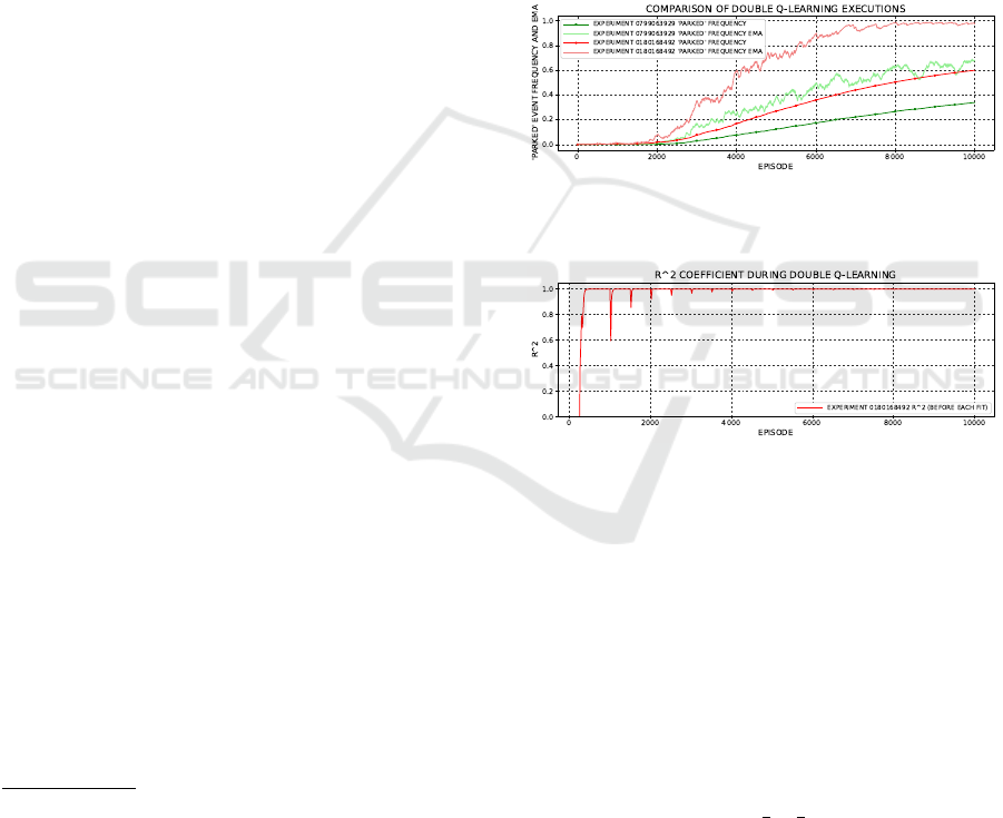
Figure 7: Comparison of two executions of double Q-

learning — experiments: 0799063929 vs. 0180168492.

Figure 8: Regression score R

(coefﬁcient of determina-

tion) for the

Q model from experiment 0180168492, plotted

along double Q-learning.

Figures 7, 8 provide example plots of: ‘parked’

event frequency, its EMA, and R

regression score

along the progress of double Q-learning for selected

experiments. The characteristic peaks present in

Fig. 8 indicate the moments where the target model

Q was switched.

Table 3 reports the aforementioned test results on

extrapolative generalization. Based on the table, one

can see how frequently the best models were able to

park successfully starting from a broader range (180

◦

)

of random angles, ψ ∼ U (

π,

π).

Finally, in Fig. 9 we demonstrate several selected

trajectories obtained by the best model (0180168492)

during: the learning stage and the two testing stages.

We also encourage the reader to see the related sample

videos available in the repository by clicking on the

presented images (README.md).

Double Q-Learning for a Simple Parking Problem: Propositions of Reward Functions and State Representations

165

Table 2: Results of parking experiments (double Q-learning and testing).

no.

experiment

hash code

reward

parameters

state

representation

ﬁnal frequency

of ‘parked’

event at

learning stage

ﬁnal EMA

of ‘parked’

event frequency

at learning stage

frequency of

‘parked’

event at

test stage

1 0378634304 1.0 0.0 0.0 avms_fb 2.04% 1.30% 0.8%

2 1228517047 1.0 0.0 0.0 dv_fb 6.03% 14.68% 10.7%

3 3783388807 1.0 0.0 0.0 dv_ﬂfrblbr 5.46% 18.34% 6.6%

4 3223156582 1.0 0.0 0.0 dv_ﬂfrblbr2s 4.65% 15.24% 9.5%

5 1712051871 1.0 1.0 0.0 avms_fb 3.52% 6.00% 7.9%

6 2561934614 1.0 1.0 0.0 dv_fb 7.20% 15.31% 3.4%

7 0821839078 1.0 1.0 0.0 dv_ﬂfrblbr 6.87% 19.87% 14.6%

8 0261606853 1.0 1.0 0.0 dv_ﬂfrblbr2s 7.50% 20.92% 25.9%

9 3085463456 1.0 1.0 1.0 avms_fb 3.49% 10.07% 5.6%

10 3935346199 1.0 1.0 1.0 dv_fb 15.55% 45.24% 34.5%

11 2195250663 1.0 1.0 1.0 dv_ﬂfrblbr 10.11% 24.66% 13.5%

12 1635018438 1.0 1.0 1.0 dv_ﬂfrblbr2s 12.63% 30.23% 33.1%

13 0799063929 1.0 2.0 4.0 dv_fb 33.86% 67.76% 65.1%

14 3353935689 1.0 2.0 4.0 dv_ﬂfrblbr 18.20% 37.67% 61.7%

15 2793703464 1.0 2.0 4.0 dv_ﬂfrblbr2s 21.00% 39.74% 25.3%

16 3390133950 1.0 8.0 16.0 dv_fb 25.44% 46.08% 52.7%

17 0986779886 1.0 8.0 16.0 dv_ﬂfrblbr 19.20% 54.06% 71.1%

18 0799450095 1.0 8.0 16.0 dv_ﬂfrblbr2s 24.39% 46.27% 57.2%

19 0719075893 1.0 4.0 2.0 dv_fb 25.64% 56.98% 43.0%

20 3273947653 1.0 4.0 2.0 dv_ﬂfrblbr 24.21% 52.50% 57.8%

21 2713715428 1.0 4.0 2.0 dv_ﬂfrblbr2s 21.55% 51.01% 46.6%

22 3468419818 1.0 16.0 8.0 dv_fb 52.55% 89.12% 87.3%

23 1065065754 1.0 16.0 8.0 dv_ﬂfrblbr 60.95% 91.31% 95.6%

24 0877735963 1.0 16.0 8.0 dv_ﬂfrblbr2s 43.07% 81.47% 92.6%

25 3497227376 1.0 32.0 8.0 dv_fb 60.64% 98.39% 99.0%

26 1093873312 1.0 32.0 8.0 dv_ﬂfrblbr 55.95% 95.68% 97.8%

27 0906543521 1.0 32.0 8.0 dv_ﬂfrblbr2s 52.75% 96.37% 96.6%

28 2686104021 1.0 32.0 8.0 dv_fb_d 49.05% 93.32% 80.2%

29 3755253765 1.0 32.0 8.0 dv_ﬂfrblbr_d 58.14% 94.19% 88.6%

30 4119951046 1.0 32.0 8.0 dv_ﬂfrblbr2s_d 57.66% 96.22% 94.8%

31 2849328398 1.0 32.0 8.0 dv_fb_da 43.98% 88.94% 94.6%

32 1633232094 1.0 32.0 8.0 dv_ﬂfrblbr_da 56.02% 95.71% 94.2%

33 0053945917 1.0 32.0 8.0 dv_ﬂfrblbr2s_da 61.35% 97.80% 98.9%

34 0937679483 1.0 32.0 8.0 dv_fb_dag 32.05% 72.47% 74.6%

35 1893399723 1.0 32.0 8.0 dv_ﬂfrblbr_dag 59.87% 91.10% 96.7%

36 0180168492 1.0 32.0 8.0 dv_ﬂfrblbr2s_dag 59.92% 97.39% 99.8%

Table 3: Extrapolative generalization: results of best mod-

els from Table 2 on a broader range (180

◦

) of initial random

angles, i.e. ψ ∼ U(

π,

π).

experiment

hash code

state

representation

frequency of ‘parked’ event

at 2nd test stage

1893399723 dv_ﬂfrblbr_dag 91.8%

1093873312 dv_ﬂfrblbr 94.5%

0053945917 dv_ﬂfrblbr2s_da 87.3%

3497227376 dv_fb 96.8%

0180168492 dv_ﬂfrblbr2s_dag 89.9%

8 ADDITIONAL EXPERIMENTS

Arbitrary Initial Positions and Angles. Having

discovered the best performing combination of: re-

ward coefﬁcients (λ

,λ

) = (1, 32,8) and state

representation dv_ﬂfrblbr2s_dag from the set of main

experiments (previous section), we performed addi-

tional experiments with more general scenes.

In the ﬁrst additional setup the park place was

ﬁxed in the middle of the scene, directed to the west:

⃗x

= (0.0,0.0),

⃗

= (−1.0,0.0); but the car’s ini-

tial position was entirely random within the region of

20 m × 20 m and with any heading angle within 360

◦

namely:

⃗x ∼ U ([−10.0,10.0] × [−10.0, 10.0]),

ψ ∼ U (0, 2π).

For reference, we preserved 10 k learning episodes,

but since the scenes became more general we

employed neural networks of larger internal ca-

pacity. The sizes of hidden layers in each

action-related substructure were doubled to become:

(512,256,128, 64). This translated onto approxi-

mately four times more network weights than before,

i.e. ≈ 1.6 M (because of dense layers). Also, we have

enlarged the batch samples in the experience replay

to the size 4 · 65 536 = 262 144. In consequence, the

time of one full experiment with 10 k episodes also

increased about four times, becoming ≈ 22 h.

The resulting model (0623865367) that we ob-

tained was able to perform complicated and very in-

teresting maneuvers, including e.g.: hairpin turns,

rosette-shaped turns, and zigzag patterns. Some of

its trajectories are illustrated in Fig. 10, for videos we

again address the reader to the repository. The suc-

cess rate for this model at test stage was 97.8% (over

1 k attempts with 25 s time limit).

Model Transfer to Rotation-Invariant State Rep-

resentation. Our second additional experiment

aimed to check if model 0623865367, described

in the previous paragraph, can be transferred to a

rotation-invariant state representation and perform

well without training on new testing scenes where not

only the car’s but also the park place’s position and

angle are arbitrary (within 20 m×20 m). More pre-

ICAART 2025 - 17th International Conference on Agents and Artiﬁcial Intelligence

166

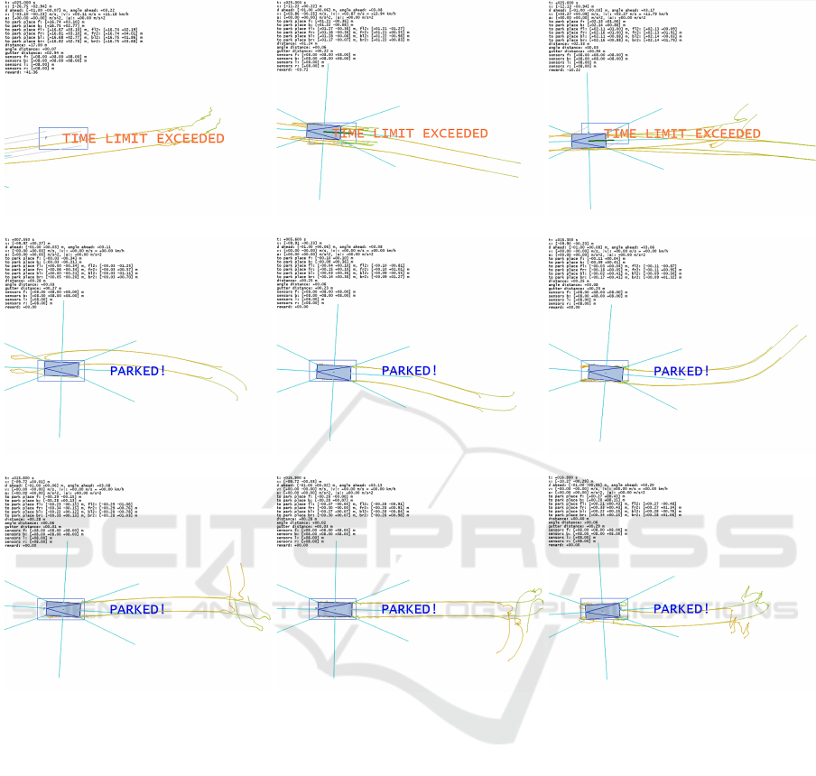
example trajectories while learning (up to episode no. 3000):

standard generalization tests (90

◦

range for initial random angles):

extrapolative generalization tests (180

◦

range for initial random angles):

Figure 9: Example trajectories at learning and testing stages (model: 0180168492).

cisely, we used the following distributions:

⃗x ∼ U ([−10.0,10.0] × [−10.0, 10.0]),

ψ ∼ U (0, 2π),

⃗x

∼ U([−10.0,10.0] × [−10.0,10.0]),

∼ U(0,2π).

The rotation-invariant state representation, called

dv_ﬂfrblbr2s_dag_invariant, can be introduced by ﬁnding

the park place rotation angle as

β = arctan2(−

⃗

) (21)

and then multiplying the vector components of

dv_ﬂfrblbr2s_dag representation by a suitable rotation

matrix at every simulation step, as shown below.

state representation

dv_ﬂfrblbr2s_dag_invariant:



M ·

⃗

d, M ·⃗v,M ·

⃗

,M ·

⃗

,M ·

⃗

,M ·

⃗

∥⃗x−⃗x

∥,φ(

⃗

d), g(⃗x)



, (22)

where

M =



cosβ −sinβ

sinβ cosβ



(23)

is the rotation matrix.

Tests carried out for the transferred model on 1 k

scenes (log ﬁle 1168277942_t.log in the repository) re-

vealed the correct and again interesting behavior of

the agent. Selected examples of maneuvering trajec-

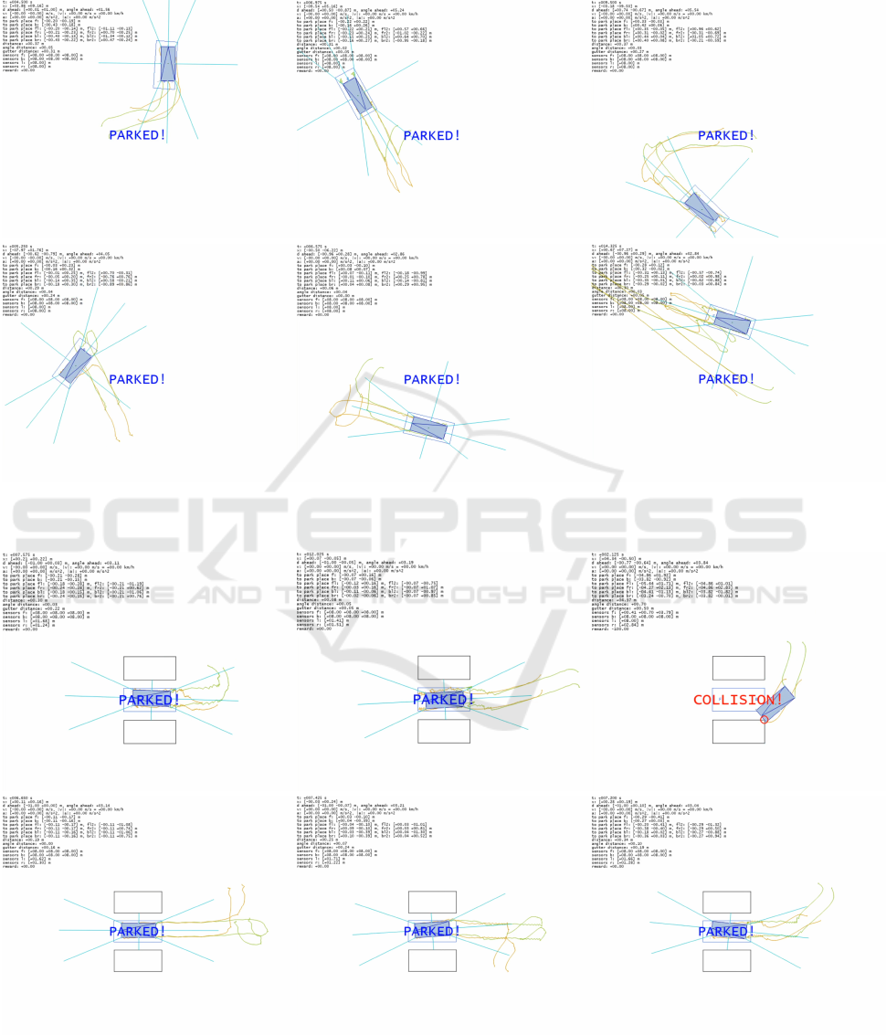
tories are illustrated in Fig. 12. The success rate we

obtained was 94.5% — slightly lower than in the pre-

vious case, but we believe still satisfactory taking into

Double Q-Learning for a Simple Parking Problem: Propositions of Reward Functions and State Representations

167

park place ﬁxed in middle,

arbitrary car position within 20 m×20 m

and arbitrary angle within 360

◦

Figure 10: Example trajectories at test stage obtained by

the model trained on scenes with arbitrary initial car posi-

tion within 20 m×20 m and angle within 360

◦

(experiment

no. 0623865367).

account the facts that the model was not trained (just

transferred) and that it was submitted to new scenes,

not experienced before, with arbitrary park place ro-

tations and positions.

Obstacles and Sensors — Preliminary Attempts.

It is natural to ask whether the proposed reward func-

tion (16) could be applicable for scenes with obsta-

cles present. A complete answer to such a question

requires a thorough analysis and more experiments,

and we plan those to be our future research direc-

tion. Nevertheless, in this paragraph we report our

very ﬁrst, preliminary attempts on this problem.

We are going to consider a scene with two obsta-

cles located sideways with respect to the target park

place — a common real-life situation where other cars

are parked in the adjacent spots. We are aware that

other arrangements of obstacles (e.g. front and rear

obstacles) might affect the results, especially having

the gutter distance in mind.

In the experiments to follow, the rotation-invariant

state representation was extended with 8 or 12 read-

ings from virtual sensors, represented graphically by

the blue beams around the car in ﬁgures, compris-

ing the total of 23 or 27 features (representation:

dv_ﬂfrblbr2s_dag_invariant_sensors). Each sensor indi-

cates the distance to the closest obstacle along its di-

rection. The maximum reading of 8.0 m indicates no

obstacle seen within that distance.

To have a referential view on the applicabil-

ity of reward function (16), we have preserved

(λ

,λ

) = (1, 32,8) — the best coefﬁcients ob-

served in former experiments. Yet, in the presence

of obstacles there is now one new element that must

be considered, i.e. a reward for collision (in fact, a

penalty). Let us denote it by r

constant. Therefore,

the new reward function is of the following form with

three cases:

r(s

′











0; if car successfully parked in s

′

; if car collided in s

′



∆t+λ

∥⃗x

′

−⃗x

∥+ λ

φ(

⃗

′

)/π+ λ

g(⃗x

′

)



(24)

It is difﬁcult to say in advance what is a good choice

for the value of r

. For the purpose of preliminary

experiments described here, we picked r

to be equal

to −10

. This choice can be treated as a guess. In

fact, it is plausible that r

should somehow depend

on (λ

,λ

). Note also that for any ﬁxed choice

of r

there shall always exist some states s

′

, suitably

deviated from the ideal target position, such that



∆t+λ

∥⃗x

′

−⃗x

∥+ λ

φ(

⃗

′

)/π+ λ

g(⃗x

′

)



< r

which implies collisions not to be the worst possible

states. Obviously, in real life one prefers not to park

than to collide.

One more mathematical detail that needs to be

discussed. It pertains to collisions and the context

of episodic tasks. Suppose r

,.. ., r

is a sequence

of rewards — realizations of R

,.. ., R

random vari-

ables, and T stands for the last time index. In our

case T = 25s/∆t = 25s/(4δt) = 250. Suppose also,

a collision takes place at time index T

. Then the dis-

counted return the agent collects ought to be calcu-

lated as:

−1

∑

t=1

t−1

∑

t=T

t−1

−1

∑

t=1

t−1

+ r

−1

− γ

1 − γ

(25)

ICAART 2025 - 17th International Conference on Agents and Artiﬁcial Intelligence

168

model transfer using rotation-invariant state representation,

arbitrary position and angle for both car and park place (within 20 m×20 m):

Figure 11: Example trajectories obtained at tests by model 0623865367 transferred to new scenes using rotation-invariant

state representation dv_ﬂfrblbr2s_dag_invariant.

park place ﬁxed in middle with 2 obstacles 1 m sideways (model 2914586007)

Figure 12: Example trajectories obtained at tests by model 2914586007 for a scene involving 2 obstacles located 1 m to the

sides of the park place.

Double Q-Learning for a Simple Parking Problem: Propositions of Reward Functions and State Representations

169

It means that although a simulation as such stops at

the collision moment, the agent keeps on receiving

constant negative rewards for collision until the end

of episode. Note that this is consistent with the zero-

valued reward for successful parking which cancels

the tail of discounted rewards in a similar manner.

In the context of double Q-learning computations and

the formula (9) for the target regression values:

∗

:= r

+ γ



′

, argmax

′

Q(s

′

;

w);



the proper handling of the future returns for terminal

states can be achieved simply by replacing the

Q(·)

response as follows

∗

:= r

+ γ · 0, (26)

∗

:= r

+ γ · r

, (27)

for the successfully parked car and the collided car,

respectively.

We now move on to the details of this addi-

tional experiment. The park place was located at

⃗x

= (0.0,0.0) and directed along

⃗

= (−1.0,0.0).

Two obstacles were adjacent sideways to it, each 1 m

away from the park place border. Random distri-

butions for the initial car position and angle were:

⃗x ∼ U([5.0,15.0] × [−5.0, 5.0]), ψ ∼ U(

π,

π) —

i.e. a range of 180

◦

. In experiments involving 8 sen-

sors, their layout was (3, 3, 1): 3 in front, 3 in the

back, 1 at each side. In experiments involving 12 sen-

sors, their layout was (3, 3, 3).

Table 4: Results of preliminary experiments on

parking with obstacles. Reward function coefﬁ-

cients: (λ

,λ

) = (1,32,8), state representation:

dv_ﬂfrblbr2s_dag_invariant_sensors, batch size for

experience replay: 262k.

no.

experiment

hash code sensors

ﬁnal frequency

of ‘parked’

event at

learning stage

ﬁnal EMA

of ‘parked’

event frequency

at learning stage

frequency of

‘parked’

event at

test stage

episodes: 10k, NN: 9 × (256,128, 64, 32)

1 0809626551 (3, 3, 1) 32.29% 60.54% 42.3%

2 0501599417 (3, 3, 3) 39.60% 68.66% 57.8%

episodes: 20k, NN: 9 × (256,128, 64, 32)

3 2914586007 (3, 3, 1) 63.72% 73.59% 80.6%

4 2606558873 (3, 3, 3) 35.33% 40.71% 69.4%

episodes: 10k, NN: 9 × (512,256, 128, 64)

5 0726961302 (3, 3, 1) 21.70% 48.25% 56.4%

6 4063022036 (3, 3, 3) 16.18% 35.23% 41.0%

episodes: 20k, NN: 9 × (512,256, 128, 64)

7 2831920758 (3, 3, 1) 38.41% 56.85% 62.0%

8 1873014196 (3, 3, 3) 41.19% 59.48% 70.4%

Table 4 summarizes the results obtained in this

preliminary experiment (example trajectories shown

in Fig. 12). Overall, the results are not satisfactory but

also not too pessimistic. Six out of 8 models managed

to perform more than 50% successful parking ma-

neuvers at the test stage in the presence of obstacles.

The best observed model (2914586007) achieved the

success rate of 80.6%. The troubling aspect is that

no clear tendencies can be seen in the results, which

makes them difﬁcult to understand. All the tested

settings (smaller / larger NNs, fewer / more sensors,

fewer / more training epsiodes) seem not to have a

clear impact on ﬁnal rates. Therefore, as mentioned

before, the general problem setting — parking with

obstacles — is planned as our future research direc-

tion.

9 CONCLUSIONS AND FUTURE

RESEARCH

Within the framework of reinforcement learning, we

have studied a simpliﬁed variant of the parking prob-

lem (no obstacles present, but time regime imposed).

Learning agents were trained to park by means of

the double Q-learning algorithm and neural networks

serving as function approximators. In this context,

our main points of attention pertained to: reward

functions (parameterized) and state representations

relevant for this problem.

We have demonstrated that suitable proportions of

penalty terms in the reward function, coupled with in-

formative state representations, can translate onto ac-

curate neural approximations of long-term action val-

ues, and thereby onto an efﬁcient double Q-learning

procedure for a car parking agent. Using barely 10 k

training episodes we managed to obtain high success

rates at the testing stage. In the main set of exper-

iments (Section 7) that rate was exceeding 95% for

several models, reaching 99% and 99.8% for two

cases.

In the additional set of experiments (Section 8) we

showed that using larger capacities of neural models

the agent was able to learn performing well in more

general scenes involving arbitrary initial positions and

rotations of both the park place and the car. In par-

ticular, the agent learned to perform complicated and

interesting maneuvers such as hairpin turns, rosette-

shaped turns, or zigzag patterns without supervision

— i.e. with being explicitly instructed about trajecto-

ries of such maneuvers.

Our future research shall pertain to a general park-

ing problem with obstacles present in the scenes and

sensor information included in state representation

(with time regime preserved). Preliminary results for

such a problem setting (Section 8) indicate the need

for more experiments and analysis. Also, it seems

appropriate to conduct in our future work a compar-

ICAART 2025 - 17th International Conference on Agents and Artiﬁcial Intelligence

170

ative evaluation of parking agents using such frame-

works as, for example, Farama

or a more general

MuJoCo

REFERENCES

Aditya, M. et al. (2023). Automated Valet Parking using

Double Deep Q Learning. In ICAECIS 2023, pages

259–264.

Cai, L. et al. (2022). Multi-maneuver vertical parking path

planning and control in a narrow space. Robotics and

Autonomous Systems, 149:103964.

Chai, R. et al. (2022). Deep Learning-Based Trajectory

Planning and Control for Autonomous Ground Vehi-

cle Parking Maneuver. IEEE Transactions on Automa-

tion and Science Engineering, 20:1633–1647.

Chen, X. et al. (2021). Independent Q-learning for Robust

Decision-Making under Uncertainty. In Proceedings

of the AAAI Conference on Artiﬁcial Intelligence, vol-

ume 35, pages 11598–11606.

Fujita, Y. et al. (2021). ChainerRL: A Deep Reinforcement

Learning Library. Journal of Machine Learning Re-

search, 22(77):1–14.

Goyal, A. et al. (2019). Modular deep reinforcement learn-

ing with functionally homogeneous modules. In Ad-

vances in Neural Information Processing Systems,

volume 32, pages 12449–12458.

Hasselt, H. (2010). Double Q-learning. In Advances in

Neural Information Processing Systems, volume 23.

Curran Associates, Inc.

Hasselt, H., van, Guez, A., and Silver, D. (2016). Deep

Reinforcement Learning with Double Q-Learning. In

Proc. of 30th AAAI Conf. on AI, pages 2094–2100.

Kingma, D. and Ba, J. (2014). Adam: A Method for

Stochastic Optimization. In ICLR (Poster). https:

//arxiv.org/pdf/1412.6980.pdf.

Kobayashi, T. and Ilboudo, W. (2021). t-soft update of tar-

get network for deep reinforcement learning. Neural

Networks, 136:63–71.

Li, Y. et al. (2018). Neural Network Approximation Based

Near-Optimal Motion Planning with Kinodynamic

Constraints Using RRT. IEEE Transactions on Indus-

trial Electronics, 65:8718–8729.

Mankowitz, D. et al. (2018). Multi-head reinforcement

learning. In Advances in Neural Information Process-

ing Systems, volume 31, pages 960–971.

Mnih, V., Kavukcuoglu, K., Silver, D., et al. (2013). Play-

ing Atari with Deep Reinforcement Learning. arXiv

1312.5602 cs.LG.

Mnih, V., Kavukcuoglu, K., Silver, D., et al. (2015).

Human-level control through deep reinforcement

learning. Nature, 518:529–533.

Nair, V. and Hinton, G. (2010). Rectiﬁed linear units im-

prove restricted Boltzmann machines. In ICML 2010,

pages 807–814.

https://github.com/Farama-Foundation/HighwayEnv

https://mujoco.org

Pedregosa, F. et al. (2011). Scikit-learn: Machine Learning

in Python. Journal of Machine Learning Research,

12:2825–2830.

Sall, R., Wagner, R., and Feng, J. (2019). Drivers’ Percep-

tions of Events: Implications for Theory and Practice.

In Proceedings of the Human Factors and Ergonomics

Society 2019 Annual Meeting, pages 1996–2000. Sage

Journals.

Shinners, P. (2011). PyGame. http://pygame.org/.

Sowerby, H., Zhou, Z., and Littman, M. (2022). Designing

Rewards for Fast Learning. arXiv 2205.15400 cs.LG.

Sprenger, F. (2022). Microdecisions and autonomy in self-

driving cars: virtual probabilities. AI & SOCIETY,

37:1–16.

Sutton, R. and Barto, A. (2018). Reinforcement Learning:

An Introduction. Bradford Books, 2 edition.

Thrun, S. and Schwartz, A. (1993). Issues in using function

approximation for reinforcement learning. In Pro-

ceedings of the 1993 Connectionist Models Summer

School.

Zeng, D. et al. (2019). A uniﬁed optimal planner for au-

tonomous parking vehicle. Control Theory and Tech-

nology, 17:346–356.

Zhang, P. et al. (2019). Reinforcement Learning-Based

End-to-End Parking for Automatic Parking System.

Sensors, 19:3996.

Double Q-Learning for a Simple Parking Problem: Propositions of Reward Functions and State Representations

171