Deep Learning for Image Analysis and Diagnosis Aid of Prostate Cancer

Maxwell Gomes da Silva

, Bruno Augusto Nassif Travenc¸olo

and Andr

e R. Backes

School of Computer Science, Federal University of Uberl

andia, Uberl

andia, Brazil

Department of Computing, Federal University of S

ao Carlos, S

ao Carlos-SP, Brazil

Keywords:

Deep Learning, Prostate Cancer, Image Segmentation.

Abstract:

Prostate cancer remains one of the most critical health challenges, ranking among the leading causes of cancer-

related deaths in men worldwide. This study seeks to automate the identiﬁcation and classiﬁcation of cancer-

ous regions in histological images using deep learning, speciﬁcally convolutional neural networks (CNNs).

Using PANDA dataset and Mask R-CNN, our approach achieved an accuracy of 91.3%. This result highlights

the potential of our methodology to enhance early detection, improve patient outcomes, and provide valuable

support to pathologists in their diagnostic processes.

1 INTRODUCTION

Prostate cancer represents a major global health chal-

lenge, ranking among the leading causes of cancer-

related mortality in men, with millions of new cases

diagnosed annually. In Brazil, it is the fourth lead-

ing cause of cancer deaths, accounting for 6% of all

cancer-related fatalities. Reports from 2022 indicate a

concerning increase, with approximately 71,730 new

cases and 16,301 deaths, representing 29.2% of male

cancer cases Humphrey (2004). Similarly, in the

United States, 2022 saw around 288,300 new cases

and 34,700 deaths, with projections indicating that 1

in 8 men will face a prostate cancer diagnosis during

their lifetime Society (2023).

In response to the rising incidence and mortal-

ity rates, Brazil and the United States have imple-

mented comprehensive cancer prevention and con-

trol policies. These initiatives focus on raising pub-

lic awareness of risk factors, promoting early detec-

tion, and ensuring equitable access to quality treat-

ment—critical steps in reducing the disease’s burden

Humphrey (2004); Society (2023).

Early detection of prostate cancer, typically

achieved through histopathological analysis of biopsy

tissue, is pivotal for effective treatment. However, this

process is inherently subjective, depending on pathol-

ogists’ expertise, and prone to variability. These lim-

itations underscore the need for computational tools

to enhance diagnostic precision and efﬁciency. Ad-

vances in artiﬁcial intelligence, particularly in con-

volutional neural networks (CNNs) and instance seg-

mentation models like Mask R-CNN, offer promising

avenues for automating the identiﬁcation and classiﬁ-

cation of histological patterns.

This study aims to develop a comprehensive

methodology for diagnosing prostate cancer through

image processing and analysis techniques. Our ap-

proach involves curating a dataset of whole slide his-

tological images and segmenting and classifying each

image based on Gleason Scores. We trained a CNN

and evaluated its performance in detecting and classi-

fying prostate cancer.

The remainder of this paper is organized as fol-

lows: Section 2 outlines the materials and methods

used in this study. Section 3 reviews related work.

Section 4 details our prostate cancer classiﬁcation ap-

proach based on Gleason Scores. Section 5 presents

and discusses the results. Finally, Section 6 concludes

the paper.

2 THEORETICAL BACKGROUND

2.1 Prostate Cancer and Gleason Score

Prostate cancer is a prevalent malignancy that affects

the prostate gland, a small organ situated below the

bladder and in front of the rectum in men. The dis-

ease occurs when cells in the prostate grow uncon-

trollably, forming tumors that may eventually spread

to other parts of the body. Risk factors include age,

family history, and certain genetic mutations. While

prostate cancer often progresses slowly, some forms

Gomes da Silva, M., Travençolo, B. A. N. and Backes, A. R.

Deep Learning for Image Analysis and Diagnosis Aid of Prostate Cancer.

DOI: 10.5220/0013302400003912

Paper published under CC license (CC BY-NC-ND 4.0)

In Proceedings of the 20th International Joint Conference on Computer Vision, Imaging and Computer Graphics Theory and Applications (VISIGRAPP 2025) - Volume 3: VISAPP, pages

699-706

ISBN: 978-989-758-728-3; ISSN: 2184-4321

699

can be aggressive and advance rapidly, making early

detection critical for effective management and treat-

ment.

Diagnosis typically involves a histopathological

examination of prostate biopsy tissue, recommended

when abnormalities are identiﬁed through digital rec-

tal examinations or elevated Prostate-Speciﬁc Anti-

gen (PSA) levels Loeb et al. (2014). The Gleason

score, derived from histopathological assessments,

evaluates the cancer’s histological grade, aiding in

predicting tumor growth rate, and metastatic poten-

tial, and guiding patient treatment plans Brazil (2002).

The National Cancer Institute classiﬁes prostate

cancer on a Gleason grading scale ranging from 1 to

5 Humphrey (2004):

• Grade 1 - Cells are uniform and small, forming

regular glands with minimal variation in size and

shape. The margins are well-deﬁned, and cells are

densely clustered with minimal stroma between

them.

• Grade 2 - Cells exhibit more variation in size and

shape, though the glands remain relatively uni-

form. Nodules are loosely arranged with irregular

borders.

• Grade 3 - Cells display greater variability in size

and shape, forming small, irregularly distributed

glands that may be angled or elongated. Spindle-

shaped or papillary nodules with smooth borders

may also be present.

• Grade 4 - Many cells merge into large, amorphous

masses or irregular glands unevenly distributed.

Signs of inﬁltration and invasion into adjacent tis-

sues are apparent.

• Grade 5 - Tumor cells are anaplastic, aggregating

into large clumps that invade nearby organs and

tissues. Central necrosis may be observed, often

with a comedocarcinoma pattern. Glandular dif-

ferentiation is frequently absent, and growth may

appear cord-like or loosely arranged, indicating

inﬁltration.

The diagnostic process relies on analyzing biopsy

tissue images and assigning a Gleason score to clas-

sify the histological grade of the tumor. Currently,

this analysis is performed manually by specialists—a

time-intensive process prone to human error. How-

ever, with advancements in cancer diagnostic tech-

nologies, there is signiﬁcant potential to develop al-

gorithms capable of identifying cancer-prone regions

and classifying them based on the Gleason score. Ex-

isting algorithms have shown promise, achieving ac-

curacy rates exceeding 77% in cancer classiﬁcation

based on known disease characteristics from medical

reports Bulten et al. (2022).

2.2 Mask R-CNN for Instance

Segmentation

An Artiﬁcial Neural Network (ANN) is a highly par-

allel, distributed processor comprising simple pro-

cessing units that store experimental knowledge and

make it accessible for practical applications Ro-

drigues et al. (2022). Similar to the human brain,

an ANN acquires knowledge from its environment

through a learning process and stores this knowledge

in the connections between neurons Haykin (1998).

Extending this concept, the Convolutional Neural

Network (CNN) draws inspiration from the brain’s hi-

erarchical feature-learning mechanisms Ghose et al.

(2012).

A CNN is structured around three primary types

of layers:

• Convolutional Layer: Performs convolution oper-

ations to extract feature maps.

• Pooling Layer: Reduces the spatial dimensions of

feature maps while retaining critical information,

improving computational efﬁciency, and reducing

overﬁtting.

• Fully Connected Layers: Transforms feature

maps into a format suitable for classiﬁcation, al-

lowing the network to categorize input data into

different classes Kang and Wang (2014).

Instance segmentation, a crucial challenge in com-

puter vision, involves accurately identifying and lo-

calizing objects within an image at the pixel level. A

leading approach for this task is the Mask R-CNN

algorithm, a state-of-the-art neural network speciﬁ-

cally designed for object detection and segmentation.

Mask R-CNN excels in distinguishing multiple ob-

jects within an image and generating bounding boxes

and pixel-level masks for each Chiao et al. (2019).

Mask R-CNN operates using a two-stage frame-

work:

• Proposal Generation: Identiﬁes Regions of Inter-

est (ROIs) within the input image where objects

of interest may exist.

• Detailed Reﬁnement: Reﬁnes these proposals

by predicting object classes, adjusting bounding

boxes, and generating precise pixel-level masks

for each ROI Gonzalez and Woods (2008).

In this study, we used the Mask R-CNN structure

implemented within the Detectron2 framework Wu

et al. (2021), comprising the following components:

1. Backbone: A Convolutional Neural Network

(ResNet) is employed to extract features from in-

put images. ResNet’s architecture incorporates

residual blocks, enabling the training of deeper

VISAPP 2025 - 20th International Conference on Computer Vision Theory and Applications

700

networks with improved accuracy and reduced

vanishing gradients.

2. Bottleneck Blocks: These building units of

ResNet contain multiple convolutional layers, of-

ten incorporating shortcuts to streamline informa-

tion ﬂow. The bottleneck blocks enhance feature

extraction across various abstraction levels.

3. Regions of Interest (ROI): After feature extraction

by the backbone, the model identiﬁes speciﬁc re-

gions within the image that may contain objects

of interest. These regions are marked for further

analysis.

4. Prediction Heads: Dedicated prediction heads are

used to perform distinct tasks within the ROIs:

• Class Prediction: Identiﬁes the class of objects.

• Bounding Box Prediction: Determines the co-

ordinates of bounding boxes surrounding de-

tected objects.

• Mask Prediction: Generates pixel-level masks

that delineate the precise boundaries of each

object.

These components synergistically enable Mask R-

CNN to perform object detection and segmentation,

from initial feature extraction to precise object iden-

tiﬁcation and localization within images. This capa-

bility makes it a powerful tool for complex computer

vision tasks.

2.3 Dataset

In our work, we used the PANDA dataset, a collec-

tion of prostate cancer biopsy images. The images

in this dataset vary in size, ranging between 21 and

50 megabytes on average, with typical dimensions of

8,192 pixels in width by 22,528 pixels in height. They

are 24-bit color images in TIFF format, requiring a to-

tal storage space of 411.9 gigabytes Kaggle (2023).

This dataset is divided into two subsets. The ﬁrst

subset, named Radboud, contains histological images

of prostate glands with detailed annotations for indi-

vidual tissue types, categorized as follows: stroma

(connective tissue or non-epithelial tissue); healthy

epithelium (benign epithelial tissue); cancerous ep-

ithelium (Gleason 3); cancerous epithelium (Gleason

4); and cancerous epithelium (Gleason 5). The second

subset, Karolinska, provides broader region-level la-

bels, deﬁned as background, non-tissue, or unknown

regions; benign tissue, a combination of stroma and

epithelial tissue; and cancerous tissue, a combination

of stroma and epithelial tissue exhibiting malignancy

Kaggle (2023).

For this study, we focused on the Radboud sub-

set due to its inclusion of additional metadata, such

as segmentation masks for each image. These masks

provide Gleason Score classiﬁcations and highlight

speciﬁc regions indicating the presence of prostate

cancer, offering ﬁner granularity essential for our

analysis and model training.

3 RELATED WORK

In recent years, numerous automatic segmentation

methods for prostate imaging in magnetic resonance

imaging (MRI) have been proposed, playing a crit-

ical role in prostate cancer management, including

detection, biopsy, staging, monitoring, and treatment

Brazil (2002); Toth et al. (2014). One such approach,

presented in LeCun et al. (2010), relies on atlas-based

region matching using contours, achieving a mean

Dice Similarity Coefﬁcient (DSC) of 84.4% on the

PROMISE12 MRI dataset. Similarly, the study in

Tian et al. (2015) utilized multiple atlases, incorpo-

rating prostate volume and contour, to reﬁne initial

segmentations. By selecting the most similar atlas

to the segmented image, the method reached a mean

DSC of 84.0% on the same dataset. Another strat-

egy employed superpixels combined with a Random

Forest classiﬁer for prostate segmentation, achiev-

ing a DSC accuracy of 88.0% on the PROMISE12

dataset Humphrey (2004). A hierarchical grouping

approach with statistical analysis, described in Yan

et al. (2016), obtained an impressive DSC rate of

92.05% on a private database.

These methods are generally categorized into four

types: contour-based, region-based, classiﬁcation-

based (either supervised or unsupervised), and hy-

brid methods Ghose et al. (2012). Each has dis-

tinct advantages and challenges. For instance, region-

based methods are intuitive but require manual pa-

rameter adjustments, while contour-based methods

adapt quickly yet are sensitive to variations in prostate

shape. Classiﬁcation-based methods are accurate and

fast but demand a robust training dataset and care-

ful feature selection Ghose et al. (2012); Tian et al.

(2015); Aldoj et al. (2020).

Deep learning, particularly Convolutional Neural

Networks (CNNs), has emerged as a transformative

approach, surpassing traditional methods by directly

learning features and patterns from images. In Chiao

et al. (2019), a deep learning-based system for Glea-

son grading in prostate cancer biopsy images achieved

77% accuracy on the SICAPv2 dataset. Similar deep

learning advancements have been observed in other

medical imaging domains, including breast cancer

detection through ultrasound imaging Chiao et al.

(2019) and oral cancer diagnosis from histological

Deep Learning for Image Analysis and Diagnosis Aid of Prostate Cancer

701

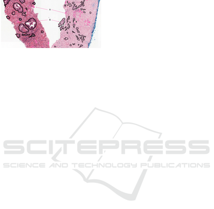
Figure 1: Example of a histological section of tissue where

morphological operations were applied. The areas outlined

in pink (A) represent the regions where these operations

were performed, resulting in the removal of certain struc-

tures. The areas outlined in black (B) represent the regions

that were preserved and considered for calculating the Glea-

son Score.

images dos Santos et al. (2023, 2021). These develop-

ments underscore the growing efﬁcacy of automated

systems in enhancing diagnostic precision and efﬁ-

ciency across medical imaging tasks.

4 EXPERIMENTAL SETUP

To prepare the images for analysis, we began by per-

forming morphological operations aimed at noise re-

duction, eliminating objects smaller than 100 pix-

els, and ﬁlling in gaps within objects up to 25 pix-

els in size Lu et al. (2019). Subsequently, we gen-

erated masks by segmenting image annotations and

assigning distinct colors to represent various cate-

gories: background (black), stroma (gray), healthy

epithelium (blue), cancerous epithelium with Gleason

Grade 3 (yellow), cancerous epithelium with Gleason

Grade 4 (red), and cancerous epithelium with Glea-

son Grade 5 (green). These masks were instrumental

in delineating object boundaries and excluding empty

regions from the dataset. Figure 1 illustrates the out-

comes of these morphological operations and the re-

ﬁnement of segmentation.

The morphological operations were pivotal in im-

proving the quality of image masks by enhancing ob-

ject contours and removing irrelevant components.

We applied a small-object removal process to ﬁlter

out regions with areas below a predetermined thresh-

old, effectively eliminating noise and artifacts that

could hinder the analysis. Following this, the remain-

ing connected regions were reprocessed and labeled

for further analysis. To visually emphasize signiﬁ-

cant regions, we extracted and overlaid contours onto

the original images, providing a clear representation

of segmented areas and their adjustments. This step,

as demonstrated in Figure 1, was essential for reﬁn-

ing the segmentation and ensuring the accuracy of the

dataset.

The processed images and masks were then di-

vided into patches measuring 512 × 512 pixels. We

retained only patches containing objects deﬁned by

the masks. To ensure a balanced dataset, we identiﬁed

the category with the fewest items and randomly se-

lected additional items from other categories to match

this number. This resulted in a total of 28,309 sam-

ples, with each category comprising 5,661 items. Fig-

ure 2 depicts the ﬁnal output of the preprocessing

stage, illustrating the uniform distribution of samples

across categories.

We structured the resulting database in the COCO

(Common Objects in Context) format, which is

widely used in machine learning for object classiﬁ-

cation and segmentation tasks Tsung-Yi Lin (2015).

This format facilitated the creation of classiﬁcation

categories corresponding to Gleason Scores and re-

gions, alongside masks for training convolutional

neural network (CNN) models.

For segmentation, we employed the Mask R-

CNN implementation from Detectron2, using lizing

a ResNet-50 backbone pre-trained on ImageNet Kyle

and Hricak (2000). The training process involved a

batch size of 12, AdamW optimizer and a learning

rate of 0.0001. We allocated 80% of the images for

training and 20% for validation. We conducted train-

ing over 40,000 iterations (approximately 22 epochs),

with learning rate reductions applied at 70% and 90%

of the training duration, halving the learning rate at

these points to optimize convergence.

Hyperparameter choices were based on both ex-

perimental results and established literature, aiming

to tailor the model’s performance to our speciﬁc

dataset. Initially, we employed Detectron2’s default

settings and subsequently loaded a pre-conﬁgured ﬁle

containing parameters optimized for our task Wu et al.

(2019); He et al. (2016); Szegedy et al. (2016).

To maintain a balanced dataset, we randomly se-

lected images and their corresponding masks across

all Gleason Score categories, ensuring the number of

samples in each category matched the one with the

fewest samples. This approach allowed us to create

a homogeneously distributed dataset, essential for un-

biased model training.

Quantitative metrics are essential to assess model

performance and guide subsequent adjustments.

These metrics measure, compare, and track model

performance, and allow for the evaluation and con-

tinuous improvement of algorithms. In our study, we

used four main metrics to assess model behavior and

generalization ability. They are:

Accuracy: measures the proportion of correct predic-

tions relative to the total number of predictions:

VISAPP 2025 - 20th International Conference on Computer Vision Theory and Applications

702

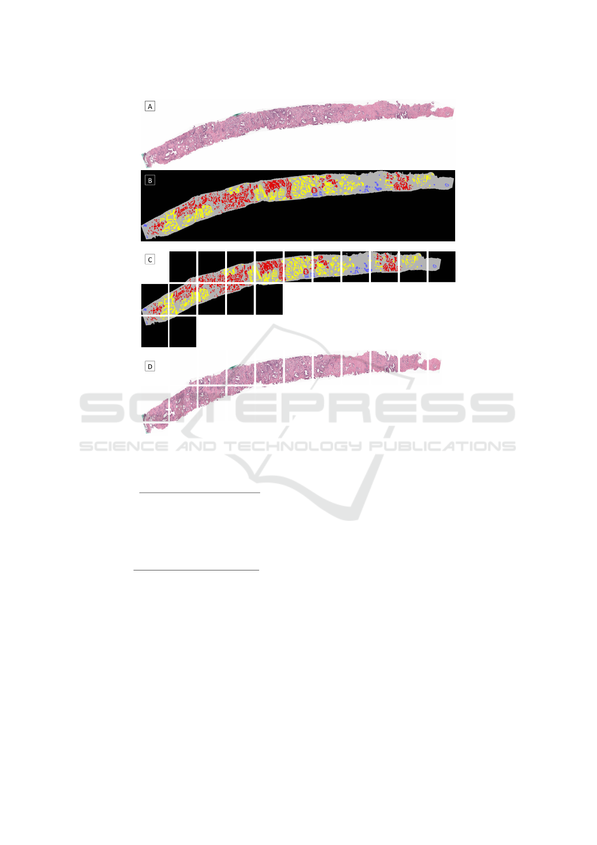
Figure 2: Example of preprocessing: A) Original image; B) Mask detected through annotations available in the dataset; C)

Mask segmented into regions with objects; D) Original image segmented by the same regions as its mask.

Accuracy =

Number of correct predictions

Total number of predictions

(1)

False Negative Rate: is the proportion of actual in-

stances of a class that were incorrectly classiﬁed as

not belonging to the class:

FNR =

False Negative

True positives + False Negative

(2)

Classiﬁcation Loss: measures the difference be-

tween the model’s class predictions and the actual

classes. It is usually calculated using cross-entropy:

Classiﬁcation Loss = −

∑

i=1

log( ˆy

) (3)

where y

is the actual class and ˆy

is the predicted

probability for the class i.

Mask Loss: measures the difference between pre-

dicted and actual binary masks, and is used to adjust

the accuracy of object segmentations in images:

mask

= BCE(

M, M) (4)

where L

mask

represents the “Mask Loss”, BCE is the

abbreviation for “Binary Cross-Entropy Loss”,

M is

the predicted mask and M is the ground truth mask.

5 RESULTS AND DISCUSSION

Figure 3 illustrates the model’s accuracy throughout

its training process, which is a key metric reﬂect-

ing the model’s ability to correctly classify images.

This ability is essential for ensuring the reliability of

the system in practical clinical applications. In our

study, we achieved a signiﬁcant accuracy of 91.34%

in identifying prostate cancer within the dataset. Fur-

thermore, the features learned by the network demon-

strated strong generalization capabilities, with only

a 0.68% difference in accuracy between the training

and validation datasets.

Figure 4 shows the percentage of false negatives

identiﬁed by the model. The false negative rate is

Deep Learning for Image Analysis and Diagnosis Aid of Prostate Cancer

703

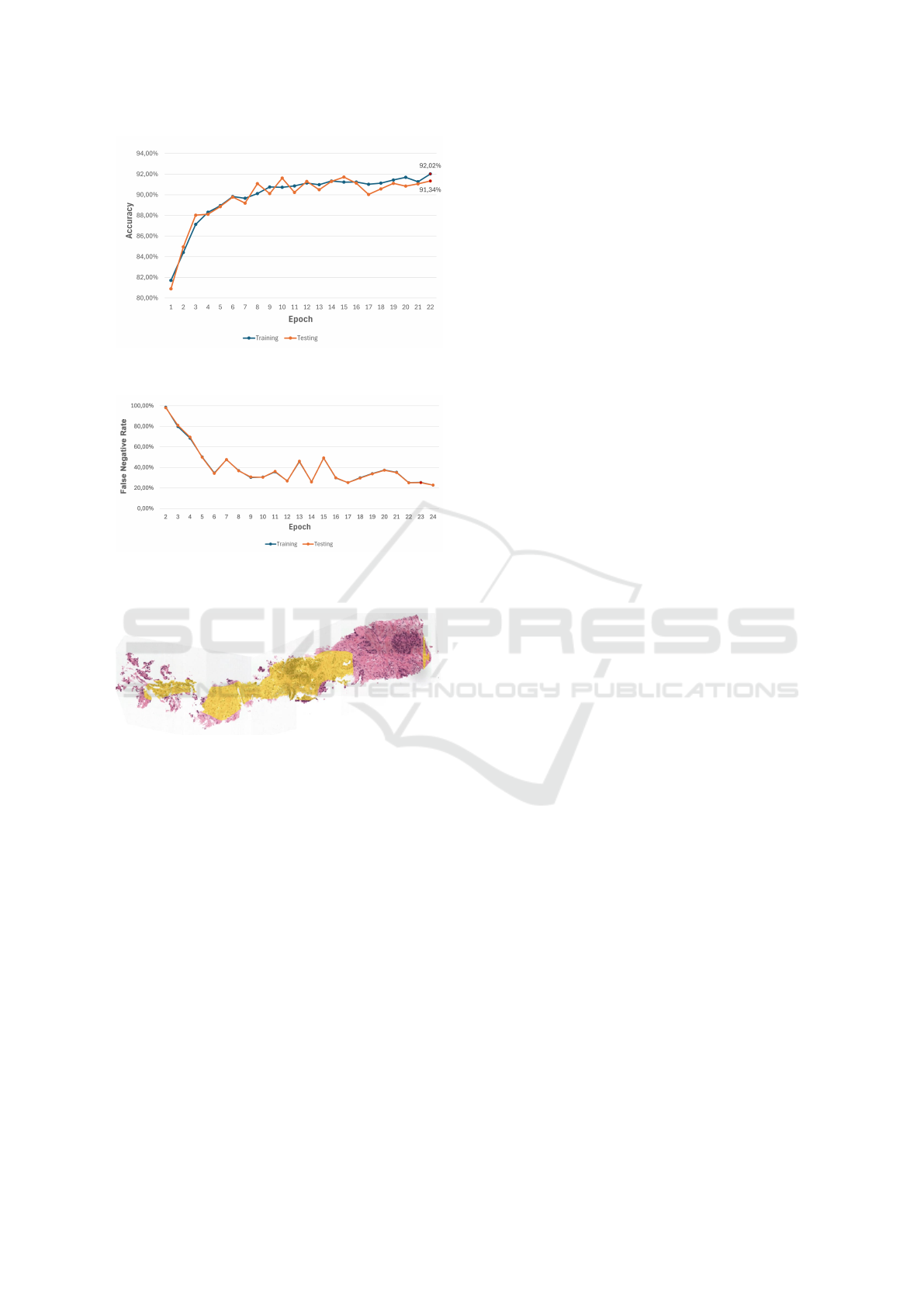
Figure 3: Accuracy of the model throughout its training pro-

cess.

Figure 4: False Negative Rate of the model throughout its

training process.

Figure 5: Example of an image with a region segmented by

the algorithm of this study.

critical, especially in applications where the conse-

quences of an incorrect prediction can be severe, such

as medical diagnosis or fraud detection.

Table 1 details the results obtained for the classi-

ﬁcation and segmentation tasks over the training and

validation. We present the loss function associated

with the classiﬁcation task, allowing us to analyze

how well the model ﬁts the training data and its poten-

tial performance on unseen data. We observe a high

initial loss in the ﬁrst epoch (441.49 in training and

448.49 in validation), which is expected at the begin-

ning of the model ﬁtting process. As the epochs pass,

the classiﬁcation loss decreases dramatically, stabiliz-

ing at around 0.39 on the training set and 0.40 on the

validation set by the last epoch. This consistent re-

duction in loss suggests that the model ﬁts the data

effectively, improving its overall performance.

Furthermore, Table 1 also reveals the values of the

speciﬁc loss function for the segmentation task. Sim-

ilar to the classiﬁcation loss, the segmentation loss is

initially high (1.07 in training and 1.09 in validation

in the ﬁrst epoch). However, this loss reduces signiﬁ-

cantly over the epochs, reaching 0.22 and 0.22 in the

last epoch for the training and validation sets, respec-

tively. The drastic reduction in the segmentation loss

over the epochs indicates a substantial improvement

in the model’s ability to correctly segment the inputs,

which is crucial for applications where accurate and

detailed segmentation is required.

In Figure 5, we present a case where Gleason

Grade 3 is clearly evident. The yellow mask overlays

a region indicative of a potential cancerous area with

a Gleason Grade of 3. These preliminary results sug-

gest that there is signiﬁcant potential for further reﬁn-

ing our methodology and improving the algorithm to

achieve even greater accuracy and performance.

Comparing the results obtained with previous

studies is essential to assess the progress made and

identify areas for future improvements. Unfortu-

nately, the literature lacks studies of this nature

with the PANDA dataset. Previous studies, such

as those conducted by Silva-Rodr

ıguez et al. (2020)

and Arvaniti et al. (2018), have sought to classify

prostate cancer according to the Gleason scale and

have demonstrated the effectiveness of deep learning-

based approaches for the detection and classiﬁcation

of prostate cancer in histopathological images. In

Silva-Rodr

ıguez et al. (2020), the authors developed a

proposal to assist pathologists in prostate slide analy-

sis. The work ranged from predicting Gleason grades

at the pixel level to detecting speciﬁc patterns, such

as cribriforms, to assessing the distribution of grades

in the tissue, leading to a biopsy score. The system

was based on deep learning for the Gleason Score

of prostate cancer biopsy images, using the SICAPv2

dataset, composed of 182 images, achieving an accu-

racy of 77% and reported to outperform existing state-

of-the-art methods.

In Bulten et al. (2022) authors report the results of

PANDA dataset competition. Most participants relied

on neural network architectures (such as Efﬁcient-

Net and ResNeXt variants), different data preprocess-

ing approaches, and automated label cleaning to per-

form image classiﬁcation. They also used ensembles

of multiple models, where different CNN models are

combined or the same model is trained using different

hyperparameters (such as loss function) or patch se-

lection strategies. Unfortunately, results are reported

using quadratically weighted Kappa (95% conﬁdence

interval) on the internal validation set (0.940), which

makes it impossible to compare with ours.

Moreover, this study builds upon a strong founda-

VISAPP 2025 - 20th International Conference on Computer Vision Theory and Applications

704

Table 1: Training and Validation results by epoch.

Epoch Accuracy (%) False Negative Rate (%) Classiﬁcation Loss Mask Loss

Training Validation Training Validation Training Validation Training Validation

1 61.39 62.36 66.47 67.52 441.49 448.49 1.07 1.09

2 83.17 82.74 98.61 98.11 37.46 37.26 0.68 0.68

3 83.63 84.96 79.79 81.06 0.72 0.74 0.46 0.47

4 86.66 88.03 68.45 69.53 0.65 0.66 0.35 0.36

5 88.72 88.12 50.17 49.84 0.68 0.67 0.34 0.33

6 89.79 88.86 34.52 34.16 0.56 0.56 0.28 0.28

7 89.47 89.78 47.59 47.75 0.62 0.62 0.28 0.28

8 89.71 89.19 36.94 36.73 0.59 0.59 0.27 0.27

9 89.79 91.09 30.28 30.71 0.52 0.53 0.26 0.26

10 90.47 90.11 30.59 30.46 0.49 0.49 0.25 0.25

11 90.43 91.62 35.70 36.17 0.49 0.50 0.25 0.26

12 90.75 90.23 26.89 26.74 0.46 0.45 0.24 0.24

13 90.50 91.30 45.74 46.14 0.54 0.55 0.29 0.29

14 90.84 90.49 25.99 25.89 0.47 0.47 0.24 0.24

15 90.95 91.30 49.10 49.28 0.61 0.61 0.29 0.29

16 91.20 91.72 29.80 29.97 0.46 0.46 0.25 0.25

17 91.15 91.13 25.23 25.23 0.45 0.45 0.23 0.23

18 91.07 90.03 29.98 29.64 0.55 0.55 0.26 0.26

19 91.25 90.57 34.02 33.77 0.49 0.48 0.25 0.25

20 91.52 91.11 37.41 37.24 0.59 0.59 0.27 0.27

21 91.52 90.84 35.31 35.05 0.49 0.49 0.26 0.26

22 91.50 91.06 25.16 25.04 0.42 0.42 0.23 0.23

23 91.97 91.34 25.36 25.19 0.43 0.43 0.23 0.23

24 91.60 91.82 22.78 22.83 0.39 0.40 0.22 0.22

25 91.03 92.23 19.59 19.84 0.36 0.37 0.19 0.20

tion by demonstrating the effectiveness of deep learn-

ing techniques in enhancing the diagnostic process of

histopathological images. The results suggest an ef-

ﬁcient learning mechanism, capable of generalizing

well to validation data. The next steps involve exper-

imenting with different neural network architectures

and validating the model on datasets like PANDA to

further reﬁne its performance for clinical applications.

This will enable us to expand the model’s generaliza-

tion capabilities in clinical contexts.

6 CONCLUSIONS

Prostate cancer is the most prevalent malignancy

among men, with rising rates of both incidence and

mortality worldwide. The Gleason Score, a critical

metric for assessing the histological grade of prostate

cancer, is essential in guiding therapeutic decisions

and predicting disease progression. Addressing the

growing need for efﬁcient diagnostic tools in pub-

lic health, this study presented an approach that in-

tegrates image processing techniques and Convolu-

tional Neural Networks to analyze prostate biopsy

images, facilitating the automation of Gleason Score

segmentation and classiﬁcation. The study achieved

a high accuracy of 91.34%, underscoring the po-

tential of this approach in prostate cancer diagno-

sis. Our approach enhances the precision and efﬁ-

ciency of prostate cancer diagnostics, enabling earlier

detection and, consequently, improving patient out-

comes. Gleason Score automated analysis reduces

the reliance on subjective manual interpretation and

speeds up the diagnostic process. In future work, we

plan to evaluate other CNNs and backbones for fea-

ture extraction and to expand the datasets evaluated.

ACKNOWLEDGEMENTS

Andr

e R. Backes and B.A.N. Travenc¸olo grate-

fully acknowledges the ﬁnancial support of CNPq

(National Council for Scientiﬁc and Technological

Development, Brazil) (Grant #307100/2021-9 and

#306436/2022-1). This study was ﬁnanced in part by

the Coordenac¸

ao de Aperfeic¸oamento de Pessoal de

ıvel Superior - Brazil (CAPES) - Finance Code 001.

Deep Learning for Image Analysis and Diagnosis Aid of Prostate Cancer

705

REFERENCES

Aldoj, N., Biavati, F., Michallek, F., Stober, S., and Dewey,

M. (2020). Automatic prostate and prostate zones

segmentation of magnetic resonance images using

densenet-like u-net. Scientiﬁc reports, 10(1):14315.

Arvaniti, E., Fricker, N., Moret, M., Rupp, N., Hermanns,

T., Fankhauser, C., Wey, N., Wild, P. J., Rueschoff,

J. H., and Claassen, M. (2018). Automated gleason

grading of prostate cancer tissue microarrays via deep

learning. Scientiﬁc reports, 8(1):1–11.

Brazil (2002). Programa Nacional de Controle de C

ancer

da Pr

ostata: Documento de Consenso. INCA,

Bras

ılia, 1 edition. 1ª ed.

Bulten, W., Kartasalo, K., Chen, P., et al. (2022). Arti-

ﬁcial intelligence for diagnosis and gleason grading

of prostate cancer: the panda challenge. Nat Med,

28:154–163. Accessed on 14/02/2024.

Chiao, J.-Y., Chen, K.-Y., Liao, K. Y.-K., Hsieh, P.-H.,

Zhang, G., and Huang, T.-C. (2019). Detection and

classiﬁcation the breast tumors using mask r-cnn on

sonograms. Medicine, 98(19).

dos Santos, D. F., de Faria, P. R., Travenc¸olo, B. A., and

do Nascimento, M. Z. (2021). Automated detec-

tion of tumor regions from oral histological whole

slide images using fully convolutional neural net-

works. Biomedical Signal Processing and Control,

69:102921.

dos Santos, D. F. D., de Faria, P. R., Travenc¸olo, B. A. N.,

and do Nascimento, M. Z. (2023). Inﬂuence of data

augmentation strategies on the segmentation of oral

histological images using fully convolutional neural

networks. Journal of Digital Imaging.

Ghose, S., Oliver, A., Mart

ı, R., Llad

o, X., Vilanova, J. C.,

Freixenet, J., Mitra, J., Sidib

e, D., and Meriaudeau,

F. (2012). A survey of prostate segmentation method-

ologies in ultrasound, magnetic resonance and com-

puted tomography images. Computer Methods and

Programs in Biomedicine, 108(1):262–287. Accessed

on 11/02/2024.

Gonzalez, R. C. and Woods, R. E. (2008). Digital image

processing. Prentice Hall, Upper Saddle River, N.J.

Haykin, S. (1998). Neural networks: a comprehensive foun-

dation. Prentice Hall PTR.

He, K., Zhang, X., Ren, S., and Sun, J. (2016). Deep resid-

ual learning for image recognition. In Proceedings of

the IEEE conference on computer vision and pattern

recognition, pages 770–778.

Humphrey, P. (2004). Gleason grading and prognostic fac-

tors in carcinoma of the prostate. Mod Pathol, 17:292–

306. Published: 13 February 2004, Issue Date: 01

March 2004.

Kaggle (2023). Kaggle. https://www.kaggle.com/c/

prostate-cancer-grade-assessment. Accessed on 14

February 2024.

Kang, K. and Wang, X. (2014). Fully convolutional neu-

ral networks for crowd segmentation. arXiv preprint

arXiv:1411.4464.

Kyle, K. Y. and Hricak, H. (2000). Imaging prostate cancer.

Radiologic Clinics of North America, 38(1):59–85.

LeCun, Y., Kavukcuoglu, K., and Farabet, C. (2010). Con-

volutional networks and applications in vision. In Pro-

ceedings of 2010 IEEE International Symposium on

Circuits and Systems, pages 253–256.

Loeb, S., Bjurlin, M. A., Nicholson, J., Tammela, T. L.,

Penson, D. F., Carter, H. B., Carroll, P., and Etzioni, R.

(2014). Overdiagnosis and overtreatment of prostate

cancer. European urology, 65(6):1046–1055.

Lu, Y., Jiang, Z., Zhou, T., and Fu, S. (2019). An improved

watershed segmentation algorithm of medical tumor

image. In IOP conference series: materials science

and engineering, volume 677, page 042028. IOP Pub-

lishing.

Rodrigues, L. F., Backes, A. R., Travenc¸olo, B. A. N., and

de Oliveira, G. M. B. (2022). Optimizing a deep resid-

ual neural network with genetic algorithm for acute

lymphoblastic leukemia classiﬁcation. Journal of Dig-

ital Imaging, 35(3):623–637.

Silva-Rodr

ıguez, J., Colomer, A., Sales, M. A., Molina, R.,

and Naranjo, V. (2020). Going deeper through the

gleason scoring scale: An automatic end-to-end sys-

tem for histology prostate grading and cribriform pat-

tern detection. Computer methods and programs in

biomedicine, 195:105637.

Society, A. C. (2023). Facts & ﬁgures 2023.

https://www.cancer.org/cancer/prostate-cancer/

about/key-statistics.html. Accessed: [02 November

2021].

Szegedy, C., Vanhoucke, V., Ioffe, S., Shlens, J., and Wojna,

Z. (2016). Rethinking the inception architecture for

computer vision. In IEEE Conference on Computer

Vision and Pattern Recognition (CVPR), pages 2818–

2826.

Tian, Z., Liu, L., and Fei, B. (2015). A fully automatic

multi-atlas based segmentation method for prostate mr

images. In Medical Imaging 2015: Image Processing,

volume 9413, pages 1067–1073. SPIE.

Toth, R. J., Shih, N., Tomaszewski, J. E., Feldman, M. D.,

Kutter, O., Daphne, N. Y., Paulus Jr, J. C., Pala-

dini, G., and Madabhushi, A. (2014). Histostitcher™:

An informatics software platform for reconstructing

whole-mount prostate histology using the extensible

imaging platform framework. Journal of Pathology

Informatics, 5(1):8.

Tsung-Yi Lin, M. (2015). Microsoft coco: Common objects

in context. Computer Vision and Pattern Recognition

(cs. CV), 1405.

Wu, Y. et al. (2021). Github. https://detectron2.readthedocs.

io/en/latest/. Accessed on 23 November 2023.

Wu, Y., Kirillov, A., Massa, F., Lo, W.-Y., and Girshick, R.

(2019). Detectron2: A pytorch-based modular object

detection library. arXiv preprint arXiv:1904.04514.

Yan, K., Li, C., Wang, X., Li, A., Yuan, Y., Feng, D.,

Khadra, M., and Kim, J. (2016). Automatic prostate

segmentation on mr images with deep network and

graph model. In 2016 38th Annual international con-

ference of the IEEE engineering in medicine and biol-

ogy society (EMBC), pages 635–638. IEEE.

VISAPP 2025 - 20th International Conference on Computer Vision Theory and Applications

706