Model Characterization with Inductive Orientation Vectors
Kerria Pang-Naylor
1 a
, Eric Chen
1,2 b
and George D. Monta
˜
nez
1 c
1
AMISTAD Lab, Dept. of Computer Science, Harvey Mudd College, Claremont, CA, U.S.A.
2
Department of Computer Science, Stanford University, Stanford, CA, U.S.A.
Keywords:
Inductive Orientation Vector, Inductive Bias, Algorithmic Bias, Algorithmic Capacity, Entropic Expressivity,
Algorithmic Search Framework, Interpretable AI, Labeling Distribution Matrix.
Abstract:
As models rise in complexity, black-box evaluation and interpretation methods become critical. We introduce
estimation methods for characterizing model-theoretic quantities such as algorithm flexibility, responsiveness
to changes in training data, and ability to specialize. These methods are applicable to any black-box clas-
sification algorithm. Past theoretical work has shown how such qualities affect probability of task success,
generalization, and tendency to overfit. We perform metric estimations of interpretable models across hy-
perparameters and corroborate the metrics’ behavior with known algorithm heuristics. This work presents a
general model-agnostic interpretability tool.
1 INTRODUCTION
Machine learning practitioners face seemingly end-
less choices of models and hyperparameters. With
this, scalable methods to evaluate and interpret al-
gorithms are critical. Model-agnostic techniques –
i.e., methods approaching models as black box func-
tions – provide flexibility crucial for describing highly
complex algorithms (e.g., deep neural networks) and
straightforward model comparison (Ribeiro et al.,
2016a).
The inductive orientation vector offers one such
black-box evaluation and interpretation technique. As
a vectorized representation of a trained model’s in-
ductive bias (Mitchell, 1980), one can easily com-
pare black-box algorithms and identify model rela-
tionships (Bekerman et al., 2022). Grounded in the
algorithmic search framework (Montanez, 2017a), the
inductive orientation vector can be used to calcu-
late interpretable model characteristics, namely, en-
tropic expressivity, algorithmic capacity, and algorith-
mic bias (Bekerman et al., 2022). These metrics de-
scribe, respectively, an algorithm’s flexibility, respon-
siveness to changes in training data, and ability to spe-
cialize (Bashir et al., 2020; Lauw et al., 2019). Un-
like established model-agnostic evaluation and inter-
a
https://orcid.org/0009-0007-3329-5211
b
https://orcid.org/0000-0002-0469-3858
c
https://orcid.org/0000-0002-1333-4611
pretability methods, the inductive orientation vector
produces understandable model-theoretic metrics that
are generalizeable to entire trained model behavior.
Past work formalized the inductive orientation
vector and analyzed common algorithms’ relation-
ships based on pairwise vector distances (Bekerman
et al., 2022). However, the inductive orientation vec-
tor’s potential use as a model evaluation and charac-
terization method remains unexplored.
We present empirical estimations and analyses
of interpretable model characteristics – algorithmic
bias, algorithmic capacity, and entropic expressivity –
through the inductive orientation vector. This method
may be applied to any black-box classifier, i.e., met-
rics are estimated given only input and output data.
We ground this method by corroborating the results
of interpretable classification models like decision
trees or k-nearest neighbors with known, algorithm-
specific theoretical characteristics (Section 4). Exper-
iments over a range of algorithms and datasets also
confirm trade-off bounds between entropic expressiv-
ity and algorithmic bias (Lauw et al., 2019; Bashir
et al., 2020) that have only been shown theoretically
(Section 5). Our work presents and verifies a new
method of model-agnostic characterization.
670
Pang-Naylor, K., Chen, E. and Montañez, G. D.
Model Characterization with Inductive Orientation Vectors.
DOI: 10.5220/0013304400003890
Paper published under CC license (CC BY-NC-ND 4.0)
In Proceedings of the 17th International Conference on Agents and Artificial Intelligence (ICAART 2025) - Volume 2, pages 670-681
ISBN: 978-989-758-737-5; ISSN: 2184-433X
Proceedings Copyright © 2025 by SCITEPRESS – Science and Technology Publications, Lda.

2 BACKGROUND
2.1 Algorithmic Search Framework
The algorithmic search framework (ASF) provides
the theoretical foundation of the inductive orientation
vector and consequent model characterizations (Mon-
tanez, 2017b). The ASF is a formalization of search
through a three tuple, (Ω, T,F), the search space, tar-
get set, and external information resource. We reduce
the ASF to classification inference on n data points,
which we refer to as the holdout set H. Given all pos-
sible labelings of the n data points, a black-box clas-
sification algorithm A “searches” for labelings with
high accuracies (e.g., how close the chosen labeling
is to assigning the n elements’ true labels). Formally,
suppose we classify n data points with c categories.
Then, the search process (Ω,T, F) is defined as fol-
lows.
1. Search space (Ω) contains all possible c
n
label-
ings of the holdout set. For example, if c =
2 and n = 5, Ω contains elements (0, 0, 0, 0, 1),
(0,0,1,0,1), and so on.
2. Target set (T ) is a subset of Ω containing la-
belings with accuracies above some minimum
threshold q
min
(for example, 80%). We may en-
code this as target function t, a |T |-hot binary en-
coding vector of length |Ω| where each index in-
dicates an element’s inclusion in the target set T .
3. External information resource (F) represents
information used by the algorithm to guide its
search. In our problem, F embeds the training
data the model receives sampled from some dis-
tribution D, along with its loss or fitness function.
Ω
P
BLACK-BOX
ALGORITHM
HISTORY
ω₀, F(ω₀)
ω₃, F(ω₃)
ω₈, F(ω₈)
ω₅, F(ω₅)
ω₂, F(ω₂)
i
i − 6
i − 5
i − 4
i − 3
i − 2
i − 1
ω₆, F(ω₆)
CHOOSE NEXT POINT AT TIME STEP i
ω, F(ω)
Figure 1: ASF process (Montanez, 2017a).
Over iterations of the search, the algorithm con-
sults external resource F and its search history
˜
H to
assign a probability mass function P
i
over the search
space rating an element’s likelihood of belonging to
target set T (Figure 1). “Success” is defined by find-
ing at least one element of T during search. By the
end of the search, a probability distribution sequence
˜
P is produced (Bekerman et al., 2022). Normalizing
across all steps (given constant resource F), we de-
note the averaged probability distribution induced on
Ω as P
F
(Bekerman et al., 2022), where
P
F
:= E
˜
P,
˜
H
"
1
|
˜
P|
˜
P
∑
i=1
P
i




F
#
. (1)
2.2 Inductive Orientation Vector
Provided with the same external information, learning
algorithms are not guaranteed to generate the same
probability distribution over the search space; dif-
ferent learning architectures achieve different losses
when trained on the same data. These differences
can be attributed to an algorithm’s innate character-
istics known as its inductive bias (Mitchell, 1980).
Any black-box evaluation of an algorithm’s induc-
tive bias requires that bias is estimated with respect
to some generator of training data, D. Otherwise, al-
gorithm behavior cannot be observed. Shared model
behavior across various data-generating distributions
D suggests algorithm characteristics that are indepen-
dent of training data or its inductive bias. We estimate
the behavior on each data distribution using an induc-
tive orientation vector, P
D
, which can be thought of
as an expectation of algorithm behavior over different
training datasets F ∼ D.
P
D
:= E
D

P
F

= E
D
"
E
˜
P,
˜
H
"
1
|
˜
P|
˜
P
∑
i=1
P
i




F
##
. (2)
The inductive orientation vector is a useful proxy
for inductive bias when comparing several algorithms
on a fixed data source D. Experiments by Beker-
man et al. (2022) have shown that inductive orienta-
tion vectors confirm known relationships between al-
gorithms’ inductive biases. The inductive orientation
vector can also be used to calculate the three model-
theoretic metrics: algorithmic bias, entropic expres-
sivity, and algorithmic capacity. This use is the sub-
ject of our work.
2.2.1 Algorithmic Bias
Algorithmic bias quantifies how much an algorithm
deviates in performance from that of uniform random
sampling.
Definition 1 (Algorithmic Bias, Monta
˜
nez et al.
(2021)). Let D be a distribution over a space of in-
formation resources F and let F ∼ D. For a given D
Model Characterization with Inductive Orientation Vectors
671

and a fixed k-hot target function t,
Bias(D,t) = t
⊤
P
D
−
∥t∥
2
|Ω|
. (3)
Recall that P
D
is an averaged probability distri-
bution across Ω where probability mass indicates an
element’s expected likelihood of belonging in the tar-
get set. Letting t be a |T |-hot vector representation of
target set T , inner-product t
⊤
P
D
is equivalent to the
sum of the probability mass P
D
places on elements of
the target set. Thus, t
⊤
P
D
is the algorithm’s expected
probability of success. We then subtract the probabil-
ity of success under uniform random sampling which
is simply |T |/|Ω| = ∥t∥
2
/|Ω|.
An algorithm without algorithmic bias cannot
generalize beyond training data and will behave like
random uniform sampling (Mitchell, 1980; Monta
˜
nez
et al., 2019). Mathematically, algorithmic bias is
high when the algorithm’s inductive orientation vec-
tor points towards the target function, resulting in a
greater than uniform probability of success. There-
fore, algorithmic bias captures whether the algo-
rithm’s assumptions are biased toward or against the
task at hand.
2.2.2 Entropic Expressivity
The inductive orientation vector also determines the
entropic expressivity of an algorithm. The entropic
expressivity measures an algorithm’s ability to dis-
tribute its probability mass over the search space
(Lauw et al., 2019). Since the inductive orientation
vector represents the expected probability distribution
over the search space relative to D, its Shannon en-
tropy H(P
D
) serves as a measure of the spread of the
algorithm’s probability mass.
Definition 2 (Entropic Expressivity, Monta
˜
nez et al.
(2021)).
H(P
D
) = H(E
D
[P
F
])
= H(U)− D
KL
(P
D
∥U) (4)
where D
KL
(P
D
||U) is the Kullback-Leibler diver-
gence between the inductive orientation vector P
D
and the uniform distribution U over Ω.
The spread of probability mass on an output space
relative to a data distribution could either be due to
an algorithm’s intrinsic randomness or its nonrandom
response to data. Due to this ambiguity, entropic ex-
pressivity is often difficult to interpret in practice.
2.2.3 Algorithmic Capacity
Algorithmic capacity is defined as the maximum mu-
tual information between the algorithm and data dis-
tribution D (Bashir et al., 2020). Also known as dis-
tributional algorithmic capacity, what we call algo-
rithmic capacity is conditioned on a specific data dis-
tribution. True algorithm capacity, or an algorithm’s
general ability to learn, is the algorithm’s theoretical
supremum of algorithmic capacity over all possible
data-generating distributions (Bashir et al., 2020).
Definition 3 (Distributional Algorithmic Capacity,
Bashir et al. (2020)). For a fixed distribution D, the
algorithm capacity specific to that distribution is rep-
resented by
C
A,D
= H(P
D
) − E
D
[H(P
F
)].
The first term H(P
D
) represents the spread of
the overall probability distribution in expectation,
namely, the entropic expressivity. It measures the
“flatness” of distribution P
D
, which can result either
from averaging flat P
F
distributions or averaging to-
gether many “sharp” distributions P
F
that place mass
on different parts of Ω (Bashir et al., 2020). The
second term, P
F
, measures the expected flatness for
a given information resource F, i.e., an algorithm’s
innate stochasticity from training on the same data
F. By subtracting away the algorithm’s intrinsic ran-
domness, C
A,D
isolates the algorithm’s nonrandom
response to data.
For a deterministic algorithm, retraining on the
same data will always produce the same model pa-
rameters, making each distribution vector P
F
place all
its probability mass on a single outcome. This results
in E
D
[H(P
F
)] = E
D
[0] = 0 and causes algorithmic
capacity to equal entropic expressivity.
3 METHODS
3.1 Estimations of Inductive
Orientation Vectors
All explored metrics require precise estimation of the
inductive orientation vector. We adopt the methodol-
ogy proposed by Bekerman et al. to estimate an ex-
pected inductive orientation vector (Bekerman et al.,
2022). Full details of the procedure and its theoretical
justification can be found in their work, but we will
briefly summarize the key steps.
We assume some dataset D as a proxy for our data-
generating distribution D (Section 6 discusses proper-
ties and limitations of this approach). We first create
K subsets of D that serve as training datasets, denoted
as F
k
. We sample with replacement to form each sub-
set, ensuring that each subset comes from the same
underlying distribution while allowing for variance
ICAART 2025 - 17th International Conference on Agents and Artificial Intelligence
672

between samples. We train the binary classification
algorithm on each F
k
r times. This repeated train-
ing on each F
k
captures possible stochastic behavior
within the same training set.
After training, each model is evaluated on a com-
mon holdout set H ⊂ D to infer its inductive orienta-
tion on the holdout data. The model’s labeling of H
is represented as a one-hot encoded vector of length
|Ω| = 2
|H|
, where the “1” element corresponds to the
labeling sequence produced by the model trained on
F
k
. The average of these vectors over the r repetitions
for the same subset F
k
is denoted as P
F
k
, representing
the inductive orientation vector for that subset.
We compute the expected inductive orientation
vector P
D
by averaging the P
F
k
vectors across all K
subsets. This results in an estimate of the overall in-
ductive orientation relative to the overall dataset.
for k = 1,. .. ,K do
F
k
← Sample without replacement from
training set;
for r = 1,. .. , R do
Generate P
F
k
r
after training A on F
k
;
P
F
k
← P
F
k
+ P
F
k
r
;
end
P
F
k
← P
F
k
/R;
Store P
F
k
in LDM;
end
P
D
← Average of the columns of LDM;
return P
D
;
Algorithm 1: Generate Labeling Distribution Matrix
(LDM) and Inductive Orientation Vector (P
D
).
Algorithmic bias, entropic expressivity, and algo-
rithmic capacity are computed as in Section 2.2.
3.1.1 Experimental Parameters
In our experiments, each data subset F
k
is 15% the
size of the training dataset (which is 80% the size of
the entire dataset). We pick each holdout set H to be
5 data points from the 20% test set. This means there
are 2
5
elements in the search space Ω. We selected
100 holdout sets per dataset to obtain a confidence
interval. This results in 100 inductive orientation vec-
tors per pair of model and dataset. Bias, expressivity,
and capacity are calculated from each vector. Note
that we chose to train many inductive orientation vec-
tors rather than increasing the size of the holdout set
because the size of the inductive orientation vector
scales exponentially with the holdout set size. Rather
than choosing a single fixed target set, we generated
results with five target sets corresponding to five min-
imum accuracy thresholds:
1
/5,
2
/5,
3
/5,
4
/5, and
5
/5.
Table 1: Theoretical maximum and minimum values for ex-
pressivity, capacity, and bias of all thresholds.
Metric Minimum Maximum
Entropic Expressivity 0 5
Algorithmic Capacity 0 5
Algorithmic Bias (size 1) -0.9688 0.0312
Algorithmic Bias (size 2) -0.8125 0.1875
Algorithmic Bias (size 3) -0.5000 0.5000
Algorithmic Bias (size 4) -0.1875 0.8125
Algorithmic Bias (size 5) -0.0313 0.9688
Table 2: Summary of experiment hyperparameter ranges.
Each range entry respectively embeds hyperparameter
[minimum, maximum; and step-size].
Algorithm Parameter Range & Step
k-nearest neighbors neighbors [1,200;5]
Decision tree max. depth [1,70;5]
Linear SVC iterations [1,1000;50]
c-support SVC iterations [1,1000;50]
Logistic regression iterations [1,200;10]
Random forest max. depth [1,70;5]
Random forest estimators [1,200;5]
Adaboost estimators [1,100;5]
3.2 Maximum and Minimum Values
The minimum algorithmic capacity and entropic ex-
pressivity are 0, which occurs when the model al-
ways places all probability mass on one element of
the search space. In contrast, the maximum of both
corresponds to the Shannon entropy of a uniform dis-
tribution on the 2
|H|
= 2
5
search space, which is 5
bits.
Algorithmic bias compares model performance to
uniform sampling. For binary classification on a hold-
out size of 5 with threshold z, the probability of suc-
cess for uniform random sampling p
z
(i.e., getting at
least z labels correct) is p
z
=
1
2
5
∑
5
l=z

5
l

. The model
performance ranges from 100% to 0%. Therefore,
bias ranges from 1 − p
z
to −p
z
. See Table 1 for all
ranges.
3.3 Datasets & Algorithms
We explore classic, highly interpretable classification
algorithms. This lets us corroborate experimental re-
sults with known algorithm properties and, therefore,
more reliably ground the model evaluation technique.
For each selected algorithm, we measured algorithmic
bias, entropic expressivity, and algorithmic capac-
ity over a wide range of possible hyper-parameters.
All models were built with Scikit-learn (Pedregosa
et al., 2011). All algorithm hyperparameter choices
are shown in Table 2.
We derived metrics from each algorithm’s per-
formance on ten UCI Machine Learning Repository
Model Characterization with Inductive Orientation Vectors
673

Table 3: Summary of datasets. B.S.E. refers to the bootstrap
standard error averaged over all features (Section 6).
Dataset Size Balance |F
k
| B.S.E.
EEG Eye State 14979 0.449 1797 41.045
Random 2000 0.501 240 1.8638
Shopper’s Intention 12245 0.155 1469 3.5670
Bank Marketing 11162 0.474 1339 2.4254
Abalone 4177 0.312 501 0.0118
Car Evaluation 1728 0.922 207 0.0758
Letter Recognition 1609 0.495 193 0.1497
Obesity 2111 0.460 253 0.1186
Spam 4600 0.394 552 0.6473
Wine Quality 6497 0.754 779 0.2457
datasets (Dua and Graff, 2017) and one synthetically
generated dataset (Random). Datasets were binarized
either by thresholding the label value or by choosing
two classes. For example, we only use the letters “T”
and “U” from the Letter Recognition dataset.
4 INDIVIDUAL ALGORITHM
ANALYSIS
In this section, we analyze metrics obtained from in-
ductive orientation vector estimations on interpretable
algorithms (decision trees, random forests, and k-
nearest neighbors). We corroborate known algorithm-
specific heuristics with experimental results. Unless
noted otherwise, the described trends and analyses
generalize an algorithm’s behavior across all datasets.
However, for all tree-based algorithms, we only dis-
play results on the EEG Eye State dataset to conserve
space and for clear comparisons.
4.1 Decision Trees
Decision tree classifiers are trained by recursively
splitting data with feature boundaries that maximize
information gain. The final tree consists of decision
nodes that lead to leaf nodes representing the pre-
dicted class. Increasing a decision tree’s depth grows
its complexity and allows the algorithm to capture
more patterns in data. However, too many layers let
the decision tree “memorize” the noise of a dataset
and overfit (Bramer, 2007; Bashir et al., 2020). Many
techniques aim to prevent and correct overfitting, such
as limiting a tree’s maximum depth (Bramer, 2007).
Across all non-random datasets, we observe an
initial sharp upward trend in nontrivial threshold algo-
rithmic bias as maximum depth grows (Figure 2). At a
certain depth, typically between 5 to 10 layers, the al-
gorithmic bias plateaus. Given that algorithmic bias is
performance compared to uniform random guessing,
this trend unsurprisingly mirrors that of training and
testing accuracy (Figure 4). Heuristically, this plateau
Figure 2: Estimated algorithmic bias for decision tree on
EEG dataset, averaged over 100 trials. Shaded regions indi-
cate 95% confidence intervals.
in accuracy when varying maximum depth indicates
that the algorithm has stopped learning generalizeable
patterns and its additional layers are simply memoriz-
ing noise (Ying, 2019).
Decision trees’ entropic expressivity and algorith-
mic capacity exhibit a nearly identical upward trend
for the first 4 to 10 layers, up to around where al-
gorithmic bias begins to plateau. This increasing al-
gorithmic capacity indicates that adding layers at low
depths helps the tree respond more to changes in train-
ing data (i.e., higher mutual information between D
and model predictions). Such behavior is consistent
with general knowledge of decision trees. Increasing
a tree’s maximum depth, particularly at low layers,
increases its complexity and allows them to handle
more input varieties (Bramer, 2007). This increased
learning capacity is consistent with the identical up-
ward trend in testing and training accuracy in this 1
to 10 layer region (Figure 4). These metrics’ plateau
at a higher depth indicates that any new layers will
have exhausted learning patterns and are only learn-
ing from noise (Bramer, 2007), leaving the distribu-
tion on Ω with the same averaged entropy.
As the maximum depth of the tree increases fur-
ther, algorithmic capacity is constant or dips slightly.
Entropic expressivity, on the other hand, increases
for a few more layers before plateauing. High en-
tropic expressivity indicates that decision trees with
more layers induce an unpredictable, “flat” probabil-
ity mass over Ω.
When entropic expressivity departs from algorith-
mic capacity, we know this increased unpredictability
is due to stochasticity rather than increased model re-
sponsiveness. Recall that E
D
[H(P
F
)] is the difference
between entropic expressivity and algorithmic capac-
ity. This term captures the spread of models’ predic-
tions across repeated trainings on the same dataset F
k
ICAART 2025 - 17th International Conference on Agents and Artificial Intelligence
674

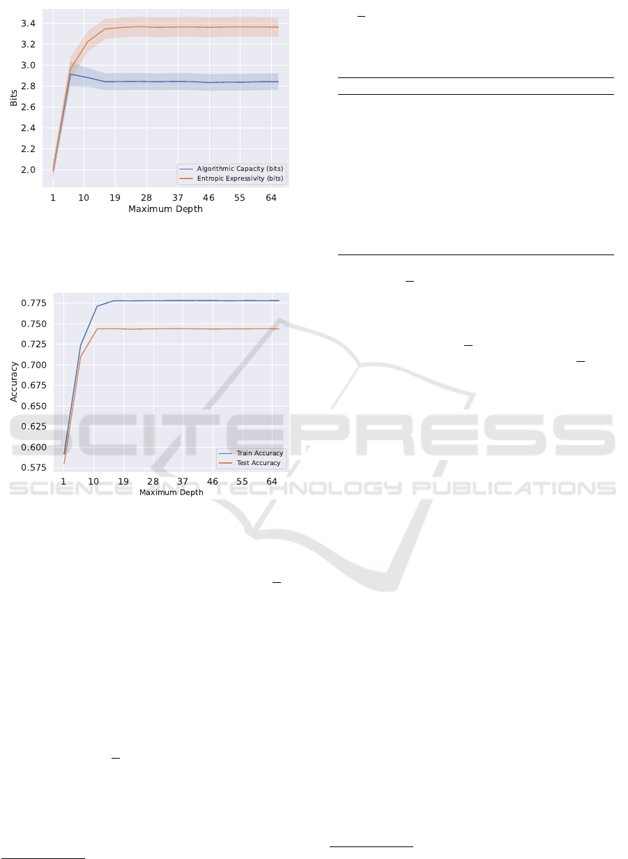
Figure 3: Estimated entropic expressivity and algorithmic
capacity for decision tree of EEG dataset, averaged over 100
trials. Shaded regions indicate 95% confidence intervals.
Figure 4: Decision tree train and test accuracies on the EEG
dataset, averaged over 100 trials. Confidence intervals are
negligible.
taken in expectation over all F
k
⊂ D. In other words, if
you retrain a model on the same dataset, E
D
[H(P
F
)]
captures how much it changes. This is the innate
stochasticity of the decision tree’s training process.
Decision trees only make random choices when there
are ties or “clashes” between alternative boundary de-
cisions due to data points with similar features but dif-
ferent outputs (Pedregosa et al., 2011; Bramer, 2007).
A popular cause of these splitting ties is overfitting,
specifically, the deeper decision nodes are trying to
learn from random noise rather than patterns (Bramer,
2007; Rong et al., 2021). Thus, increase in the aver-
age value of E
D
[H(P
F
)] could indicate overfitting.
Heuristically, non-negligible differences between
test and train accuracy may indicate overfitting (Ying,
2019). For all datasets where decision trees exceed a
test-train accuracy of 3% at any depth, we observed
overall strong and statistically significant Spearman
1
1
Spearman coefficients may be more relevant than Pear-
Table 4: Spearman and Pearson correlation coefficients of
E(H(P
F
)) vs. test-train accuracy deviation from maximum
depth values of 1 to 70. Bolded entries denote that a train-
test accuracy difference of more than 3 percent was reached.
** indicates p < 0.05, and * indicates p < 0.07 significance.
Dataset Pearson Spearman
EEG Eye State 0.9990 0.6791**
Random 0.9967 0.6923**
Shopper’s Intention 0.9988 0.9893*
Bank Marketing 0.9978 0.9626**
Abalone 0.9963 0.9963**
Car Evaluation 0.9875 0.1253*
Letter Recognition 0.7839 0.4374
Obesity 0.9907 0.2044
Spam 0.9607 0.5165*
Wine Quality -0.9759 0.2
and Pearson correlation coefficients between the esti-
mated E
D
[H(P
F
)] and the average difference between
train and test accuracy (Table 4). Overfitting and un-
derfitting are undecidable model properties (Bashir
et al., 2020; Sehra et al., 2021), but such a strong cor-
relation between E
D
[H(P
F
)] and accuracy deviations
may indicate a relationship between E
D
[H(P
F
)] and
overfitting in tree-based models.
4.2 Random Forest
Next, we analyze how decision trees behave when en-
sembled as random forests. Designed to address the
noise sensitivity of individual decision trees, a ran-
dom forest is formed by bootstrap aggregation of n
trees (i.e., the number of “estimators”). The random
forest trains n decision trees on n bootstrapped sam-
ples of the training dataset, each ignoring some ran-
domly selected subset of features. A random forest
will run any input through each of its n trees and out-
put the majority class (Parmar et al., 2019; Pedregosa
et al., 2011).
We calculated metrics for random forests when
varying both the number of estimators and the max-
imum depth of each tree. While varying depth, we
maintained the default estimator count of 100. When
varying the number of estimators, we did not impose
any pruning or maximum depth limit.
Like with individual decision trees, increasing the
maximum number of layers results in a similar up-
ward then plateauing trend for algorithmic bias val-
ues of non-trivial target threshold sizes (Figure 5).
An initial increase in model complexity allows indi-
vidual trees to capture patterns, but too many layers
let the model overfit and do not improve performance
(Bramer, 2007).
son coefficients because monotonic trends are less sensitive
to outliers compared to linear relationships.
Model Characterization with Inductive Orientation Vectors
675

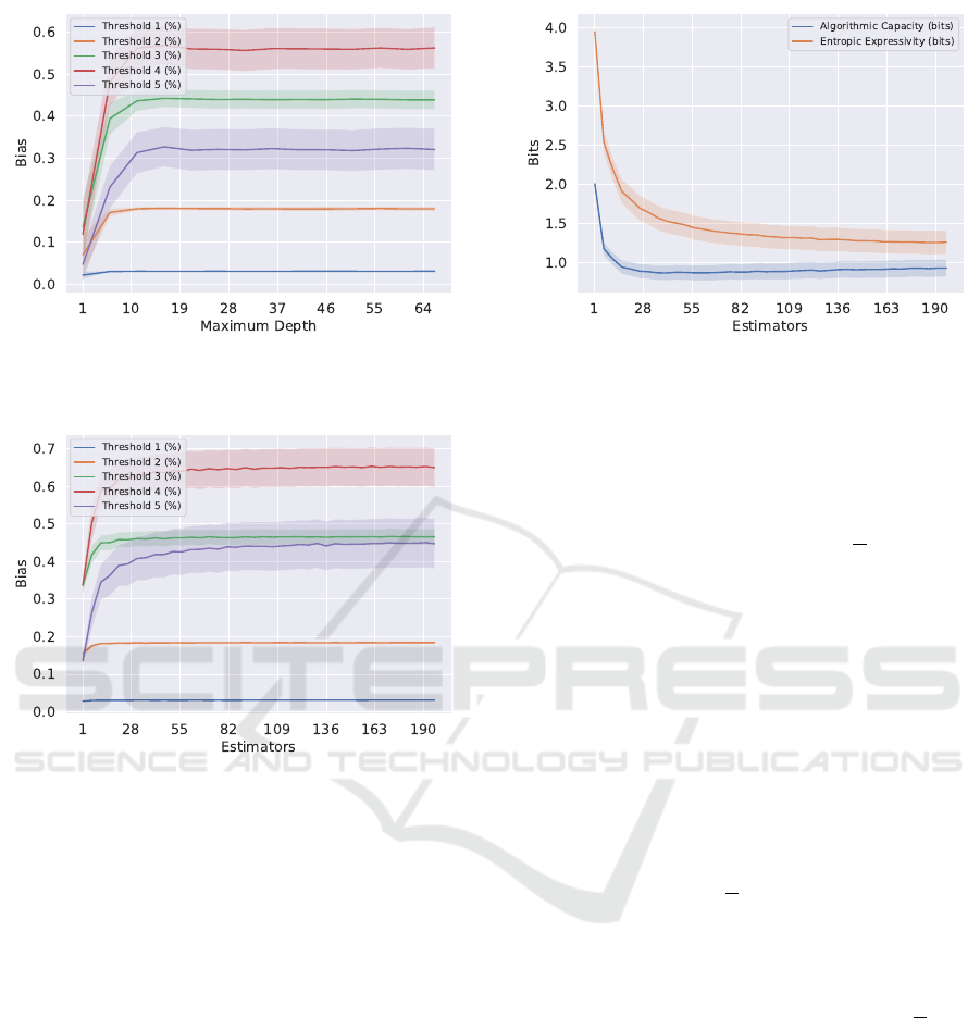
Figure 5: Random forest algorithm bias trend varying max-
imum depth (EEG dataset).
Figure 6: Random forest bias when varying estimator count
range (EEG dataset).
Increasing the number of estimators in a random
forest is generally thought to improve performance, as
more “voters” will overwhelm the few “uninformed”
trees given irrelevant features (Probst and Boulesteix,
2018). Unsurprisingly, we observe this increase in
performance and algorithmic bias over all datasets.
Typically, a sharp increase of algorithmic bias occurs
in the 1 to 20 estimator range, likely due to the forest
gaining enough decision trees to “cover” all features
of the dataset. Due to the aggregation/voting process
of random forests, the addition of one estimator can
change the overall forest output. This results in an
“even-odd” alternating pattern (Figure 6).
Aggregation with a large number of estimators
also produces a stabilizing effect on inferences. More
trees voting will cause the forest to produce more con-
sistent labelings of the holdout set and also decreases
its vulnerability to noise and overfitting (Parmar et al.,
2019). Because of this, we observe that the entropic
expressivity, i.e., the spread over the final inductive
orientation vector, decreases as the number of estima-
Figure 7: Random forest capacity and expressivity varying
number of estimators (Bank marketing).
tors increase. More specifically, a random forest with
a large number of estimators is less prone to innate
stochastic effects in outcome (Parmar et al., 2019;
Bramer, 2007). When performing repeated trainings
on the same dataset, this property causes the entropy
within individual training sets E
D
[H(P
F
)] (i.e., the
difference between expressivity and capacity) to de-
crease, and so entropic expressivity and algorithmic
capacity grow closer and the number of estimators
grows (Figure 7). The downward trend of algorithmic
capacity indicates less variation from altering train-
ing subsets F
k
⊂ D. In the context of random forests,
these trends can be interpreted as a forest becom-
ing more focused and less prone to randomness and
changes in data within D as the number of estimators
grows. This is consistent with random forests’ stabi-
lizing effect on outputs. (Parmar et al., 2019; Bramer,
2007)
Varying each estimator’s maximum depth has a
smaller effect on E
D
[H(P
F
)] than the number of esti-
mators (Figure 8). The variations between predictions
of random forest models trained on the same dataset
are mainly caused by the random feature selection
process (Parmar et al., 2019). This source of stochas-
ticity is independent of tree depth, so E
D
(H(P
F
)) is
less affected by varying tree depth. Changing the
maximum depth causes much more dramatic effects
on individual decision trees as in Figure 3. Further-
more, the algorithmic capacity and entropic expres-
sivity of random forests are consistently less than
that of individual trees across all non-random datasets
(Figure 3). This is consistent with the stabiliza-
tion that random forests provide. An ensemble of
trees will collectively react less strongly to changes
in training subsets within D and are less innately
stochastic than individual trees.
ICAART 2025 - 17th International Conference on Agents and Artificial Intelligence
676

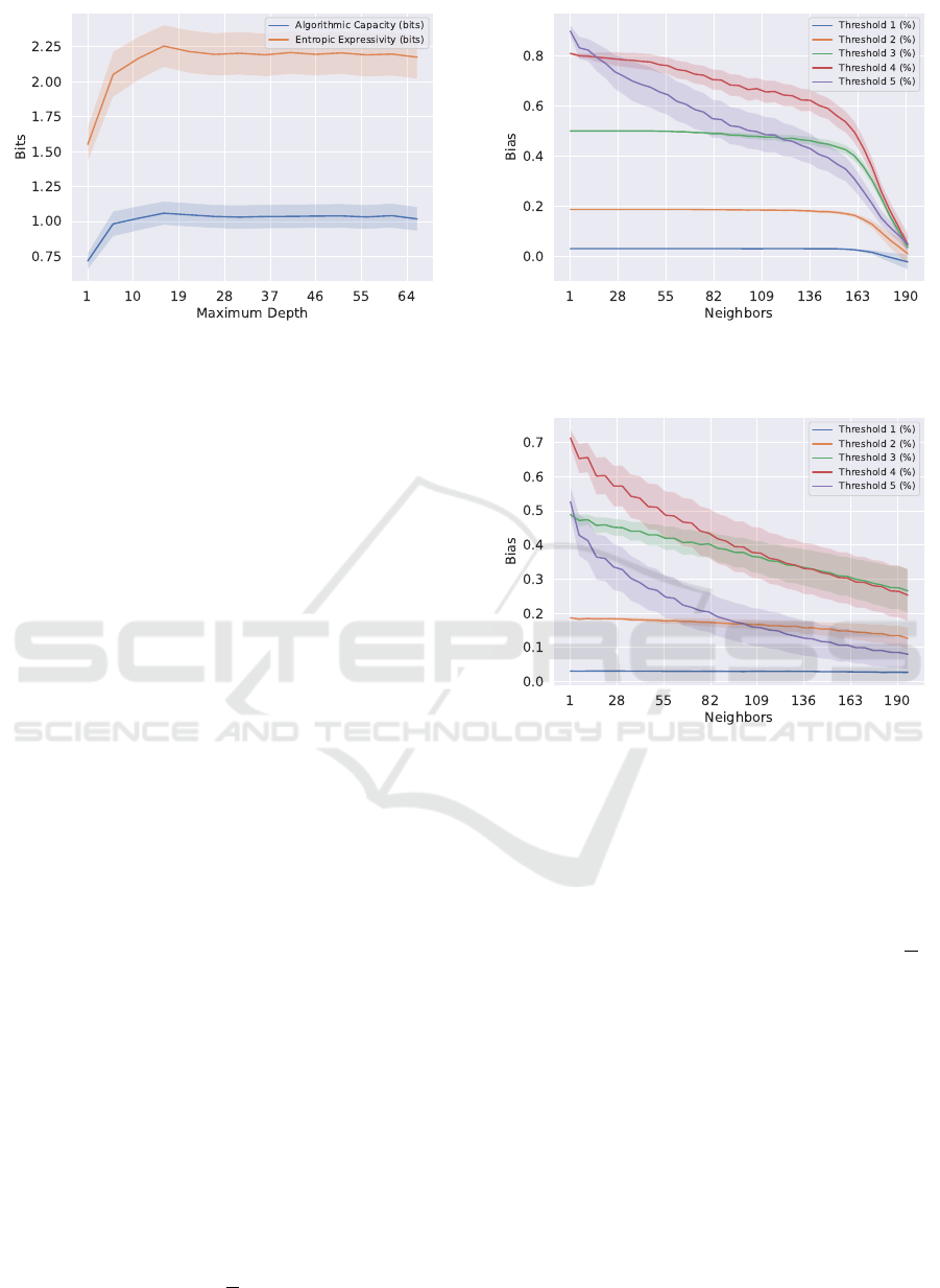
Figure 8: Expressivity and capacity of random forests var-
ied by maximum depth (EEG).
4.3 K-Nearest Neighbors
The K-Nearest Neighbors (KNN) classifier labels us-
ing the majority class of the k nearest data points to
the input feature vector. Similar to random forests,
KNN voting produces an even-odd pattern in algo-
rithmic bias (Figures 9, 10). As k grows large rela-
tive to the number of samples, the classifier resembles
majority voting and ignores local patterns (Mucherino
et al., 2009). For imbalanced datasets, majority vot-
ing labels all data the same way, and for balanced
datasets, majority voting resembles random guessing.
Both are typically more incorrect than small k voting,
so we observe an overall downward trend in bias (Fig-
ures 9, 10).
The KNN algorithm directly depends on data-
points’ locations, and so KNN classification performs
best on datasets where classes are clearly separated
in the feature-space. The modified Letter Recogni-
tion is one such dataset, as the distinct features of ‘T’
and ‘U’ characters creates distinct contiguous regions
of the feature-space. (This is confirmed by how the
linear-kernel SVC algorithm has near-perfect 0.9956
accuracy, indicating that classes are easily separable
into contiguous regions.) When trained on the mod-
ified Letter Recognition dataset, KNNs at low neigh-
bor count k nearly meet the theoretical upper limits
for algorithmic bias (see Section 5) and has >98%
test and train accuracy, likely due to Letter Recogni-
tion’s well-separated classes. As k approaches 190
or the size of its training set (Table 3), the algorithm
simply becomes majority voting on highly balanced
dataset (Table 3), and so we see a steep fall in per-
formance. This fall in performance is observed on all
other non-random datasets, such as EEG (Figure 10).
Since KNN is a deterministic algorithm (i.e.,
training a KNN on the same data always produces
sames the output), E
D
[H(P
F
)] is zero and algorith-
Figure 9: KNN algorithmic bias varying number of neigh-
bors (Letter Recognition).
Figure 10: KNN algorithmic bias varying number of neigh-
bors (EEG).
mic capacity and entropic expressivity are equivalent.
At low k, KNNs trained on any subset F
k
of the let-
ter recognition dataset have near perfect accuracy, and
place almost all probability mass on the single ele-
ment of the search space Ω representing the correct
labeling of holdout set H. This results in an ex-
tremely low entropy inductive orientation vector P
D
,
and therefore, both expressivity and capacity are near
zero at small k. As k rises, the classifier is no longer
perfect, and training on different F
k
training samples
will produce different labelings of H depending on the
majority class of each (balanced) random subset of
D. Thus, the algorithm will place probability mass on
more elements of Ω (not just the correct labeling), and
entropic expressivity and algorithmic capacity will in-
crease (Figure 12).
However, most datasets’ classes are not perfectly
separated in the feature space. This means that low
neighbor KNNs lack local class purity, resulting in
a lower starting algorithmic bias compared Letter
Recognition (Figure 10). With this “greater room
Model Characterization with Inductive Orientation Vectors
677

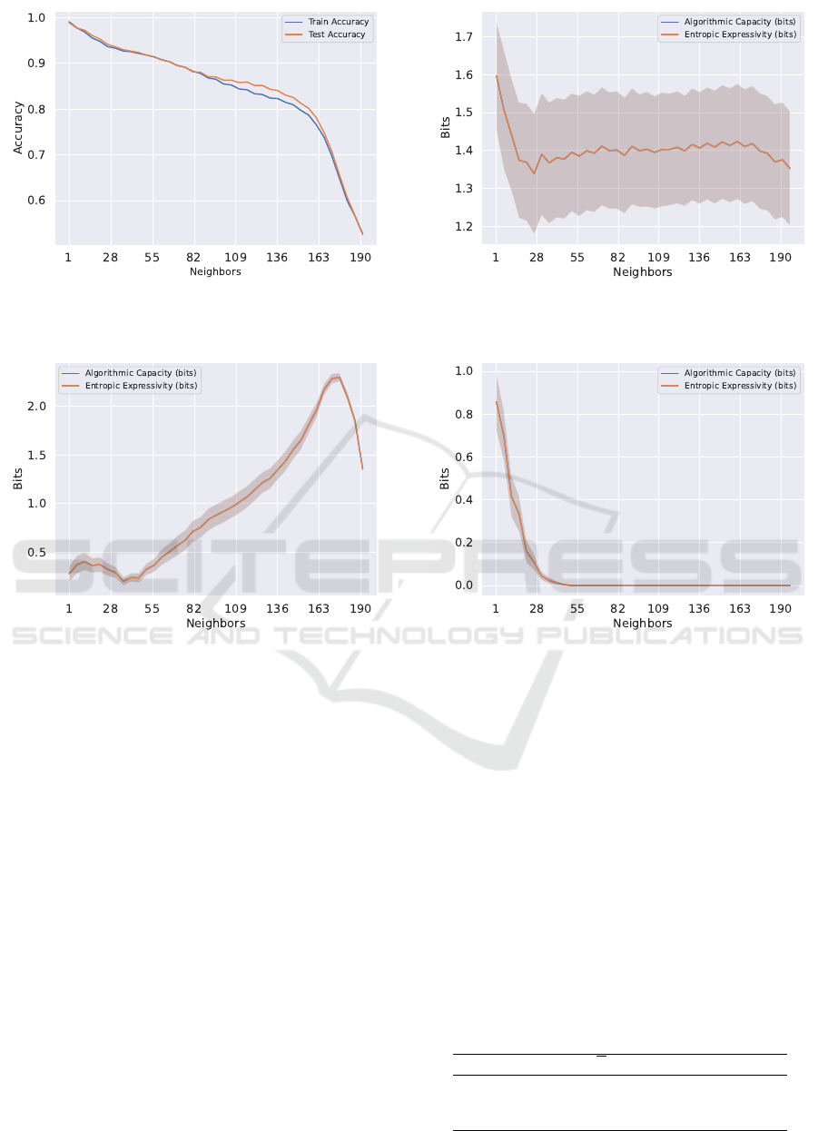
Figure 11: KNN accuracy varying number of neighbors
(Letter Recognition).
Figure 12: KNN expressivity and capacity varying number
of neighbors (Letter Recognition).
to fail”, entropic expressivity and algorithmic capac-
ity begin at much higher values compared to Letter
Recognition (Figure 13). For balanced datasets such
as EEG, expressivity and capacity do not see dramatic
changes (Figure 13). High neighbor KNNs where k
approaches the size of a balanced training set |F
k
| are
subject to the randomness of the majority class of F
k
,
and low k KNNs are subject to the local randomness
for a non-locally pure dataset.
However, the expressivity and capacity for KNNs
trained on highly imbalanced datasets like Car Evalu-
ation quickly fall to zero as k approaches |F
k
|. This is
because if k = |F
k
| (and F
k
is highly imbalanced), the
KNN algorithm will always choose the majority class
of the dataset, resulting in all probability mass placed
on the element of Ω where all five elements of H are
labeled as the majority class. Thus, the expected en-
tropy over the inductive orientation is zero, and ex-
pressivity and capacity are also zero (Figure 14).
Figure 13: KNN expressivity and capacity varying number
of neighbors (EEG).
Figure 14: KNN expressivity and capacity varying number
of neighbors (Car Evaluation).
5 THE BIAS-EXPRESSIVITY
TRADEOFF
Bashir et al. (2020) and Lauw et al. (2019) proved
trade-off bounds between algorithmic bias with both
entropic expressivity and algorithmic capacity. Intu-
itively, this tradeoff reflects how an algorithm can-
not be both very effective at one task (i.e., high bias)
while flexible for all tasks (i.e., high expressivity). If
we let p be the probability of success from random
sampling, Lauw et al. (2019) proved the following
ranges for expressivity given values of bias (Table 5).
Table 5: Varying ranges of entropic expressivity for differ-
ent levels of bias on target t where k is the target set size.
Bias(D,t) E[t
⊤
P
F
] Expressivity Range
−p (Min) 0 [0,log
2
(|Ω| − k)]
0 p [H(p),log
2
|Ω|]
1 − p (Max) 1 [0,log
2
k]
ICAART 2025 - 17th International Conference on Agents and Artificial Intelligence
678

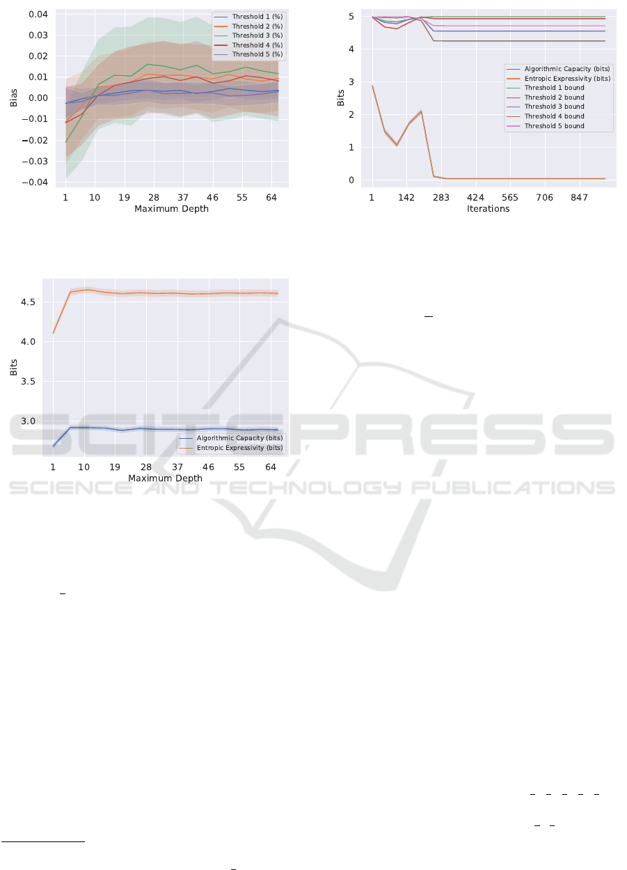
Figure 15: Random forest algorithmic bias (Random
dataset).
Figure 16: Random forest entropic expressivity and algo-
rithmic capacity (Random dataset).
Trade-off bounds are most visible where expres-
sivity and bias reach close to their theoretical lim-
its. Following the bounds from Table 5, when the
threshold
4
5
algorithmic bias of the k-nearest neigh-
bors algorithm reaches near its theoretic maximum
bias at low k (Figure 9), expressivity
2
is around 0.25
(Figure 12). Furthermore, the two figures show ca-
pacity and expressivity do not increase until bias de-
creases from its theoretical maximum (achieved by
increasing k). Similarly, when algorithmic capacity
is close to 0, expressivity obeys only the upper bound
of log
2
|Ω| = 5. For example, random forest ran on
the Random dataset has near-zero bias across all es-
timator counts and thresholds (Figure 15). As a re-
sult, entropic expressivity appears upper bounded by
5 (Figure 16).
We have also verified the direct upper bound for-
mulas for algorithmic bias and entropic expressivity
2
This is below log
2
(|T |) when |T | = 1.2, which ap-
proaches the size 1 target set of our strongest
5
5
threshold.
Figure 17: C-support SVC entropic expressivity and upper
bounds (Shopper’s Intention).
developed by Lauw et al. (2019). In our experiments,
the upper bound for algorithmic bias was consistently
above 1 (and thus trivial). The entropic expressivity
upper bound, H(P
D
) ≤ log
2
|Ω| − 2Bias(D,t)
2
, was
nontrivial for all experiments and often mirrors the
expressivity trends (Figure 17).
6 DISCUSSION & LIMITATIONS
The inductive orientation vector allows researchers to
estimate algorithmic bias, entropic expressivity, and
algorithmic capacity, which are three model-theoretic
values with established properties and behaviors (Se-
gura et al., 2019; Bashir et al., 2020; Rong et al., 2021;
Ramalingam et al., 2022; Monta
˜
nez et al., 2021). In
this section, we discuss important factors to consider
when estimating and using these metrics.
First, recall that algorithmic bias is dependent on a
minimum accuracy threshold on H which determines
whether a sequence of labels is included in the target
set. This threshold can be chosen by the experiment
setup. For a holdout size |H|, there are |H| + 1 pos-
sible thresholds and thus versions of algorithmic bias.
As the threshold lowers, the size of the target set T
approaches |Ω|, and it becomes harder for the algo-
rithm to outperform uniform random sampling. This
leads to low algorithmic bias when the threshold is
close to 0. On the other extreme, when the threshold
is near maximum (|H|/|H|), both random sampling
and trained algorithms tend to struggle, which gener-
ally causes a dip in bias. In our experiments (where
|H| = 5) we consider thresholds of
1
5
,
2
5
,
3
5
,
4
5
,
5
5
(ig-
noring the trivial 0 threshold). By the aforementioned
logic, “middle ground” thresholds of
3
5
,
4
5
tend to have
the highest bias values. It is important to generate al-
gorithmic bias based on the threshold most aligned
Model Characterization with Inductive Orientation Vectors
679

with the needed accuracy for a problem.
When interpreting the estimated algorithmic ca-
pacity of a trained model in terms of mutual infor-
mation, it is important to stress that inductive orien-
tation vectors measure distributional algorithmic ca-
pacity with respect to a training dataset D, as devel-
oped by Bashir et al. (2020). Unlike classical def-
initions of capacity, our estimated distributional al-
gorithmic capacity captures mutual information be-
tween model outputs and potential subsets within a
given training dataset. Theoretical algorithm capac-
ity posits D as a theoretical universal data-generating
distribution where sampled datasets F ∼ D may be
entirely different. Thus, for most datasets, distribu-
tional algorithmic capacity does not reflect the clas-
sical intuition that capacity is an algorithm’s “ability
to learn”. Rather, this form of algorithmic capacity
is the mutual information between a dataset’s subsets
and model behavior. In other words, how much does
knowing which subset of D was selected (i.e., the out-
come of “random variable” D) tell you about the be-
havior of the model it will train (and vice versa).
One consequence is that an extremely low entropy
dataset may produce F
k
subsets that are virtually iden-
tical and, therefore, algorithmic capacity will be zero.
For example, imagine a dataset with only two data
points repeated n times. Then, models trained on dif-
ferent F
k
subsets randomly sampled from D will be
identical and capacity will be zero. Hence, it is im-
portant to interpret algorithmic capacity with respect
to the dataset’s entropy or bootstrap variance. (Our
datasets’ averaged bootstrap standard errors are dis-
played in Table 3). Similarly, if a model’s behavior
is zero entropy, that is, the model always assigns the
labels of H to the same values, then capacity will also
be zero (this is demonstrated in the KNN behavior in
Figures 14 and 12).
To estimate true non-distributional algorithmic ca-
pacity, that is, an algorithm’s ability to learn, one must
swap each F
k
for an entire dataset generated by some
distribution. In practice, this would require synthetic
data or some large, representative data generator (e.g.,
real-time internet data).
Regarding computational constraints, the size of
the search space scales exponentially with the hold-
out set size |H|. Our method characterizes model
behavior on H, so we recommend addressing uncer-
tainty by running estimations with different randomly
sampled small holdout sets rather than increasing |H|,
as briefly mentioned in Section 3.1.1. Unfortunately,
this need for repeated inferences may be resource-
intensive for larger algorithms.
That said, these metrics have practical insights.
For example, an online learning algorithm may use
estimates of entropic expressivity and algorithmic ca-
pacity to quantify the stochasticity from the model as
opposed to its time-dependent data distribution. Our
analysis showcased connections between these met-
rics and known model behavior, suggesting predictive
abilities on general black-box algorithms. Past the-
oretical work has also proven how such qualities af-
fect model generalization and the tendency to over-
fit (Monta
˜
nez et al., 2021; Bashir et al., 2020; Rama-
lingam et al., 2022).
7 RELATED WORK
Traditional evaluation metrics such as accuracy, pre-
cision/recall, and F1 score effectively describe a mod-
els’ overall performance for a general task, but of-
fer little insight for the algorithms’ innate behav-
ior (Powers, 2020). On the other hand, model-
agnostic explainability techniques such as Local In-
terpretable Model-agnostic Explanations (LIME) and
other local estimation methods (Craven and Shav-
lik, 1995; Strumbelj and Kononenko, 2010; Baehrens
et al., 2010) use interpretable algorithms (e.g., deci-
sion trees, linear functions) to approximate a models’
underlying behavior local to an individual prediction,
but struggle when describing general model behavior
(Ribeiro et al., 2016b,a). Inductive orientation vectors
allow a middle ground between generalization and
interpretability, describing overall model behavior in
terms of information-theoretic model properties.
SHapley Additive exPlanations (SHAP) is another
model interpretation technique used to determine
which features are most influential for model output
(Lundberg and Lee, 2017). This means SHAP pro-
vides interpretability at the inference stage. In con-
trast, our approach focuses on evaluating a model’s
capacity to learn and adapt to specific problems which
is more useful for model selection.
We specifically introduce a method estimating
distributional algorithmic capacity as a proxy for
capacity or mutual information for a specific in-
putted dataset. In contrast, existing methods of es-
timating mutual information (Butakov et al., 2024)
assume a specific data distribution, and classical
methods such as applying VC dimension estimation
and Rademacher complexity provide capacity upper
bounds rather than direct estimations (Segura et al.,
2019).
ICAART 2025 - 17th International Conference on Agents and Artificial Intelligence
680

8 CONCLUSION AND FUTURE
WORK
We introduced and empirically validated model-
agnostic metrics for evaluating black-box classifica-
tion algorithms: algorithmic bias, entropic expres-
sivity, and algorithmic capacity. These information-
theoretic metrics provide interpretable insights into
model behavior. Moving forward, we hope to explore
the behavior of these metrics with non-static data and
data of varying entropy. Given the methods’ reliance
on bootstrapping and retraining, we must also test
these metric estimations on larger and more complex
algorithms and verify their practical applicability with
modern ecosystems.
REFERENCES
Baehrens, D., Schroeter, T., Harmeling, S., Kawanabe, M.,
Hansen, K., and M
¨
uller, K.-R. (2010). How to explain
individual classification decisions. The Journal of Ma-
chine Learning Research, 11:1803–1831.
Bashir, D., Monta
˜
nez, G. D., Sehra, S., Segura, P. S., and
Lauw, J. (2020). An information-theoretic perspective
on overfitting and underfitting. In AI 2020: Advances
in Artificial Intelligence: 33rd Australasian Joint Con-
ference, AI 2020, Canberra, ACT, Australia, November
29–30, 2020, Proceedings 33, pages 347–358. Springer.
Bekerman, S., Chen, E., Lin, L., and Monta
˜
nez, G. D.
(2022). Vectorization of bias in machine learning algo-
rithms. In ICAART (2), pages 354–365.
Bramer, M. (2007). Avoiding overfitting of decision trees.
Principles of data mining, pages 119–134.
Butakov, I., Tolmachev, A., Malanchuk, S., Neopryatnaya,
A., and Frolov, A. (2024). Mutual information estimation
via normalizing flows. arXiv preprint arXiv:2403.02187.
Craven, M. and Shavlik, J. (1995). Extracting tree-
structured representations of trained networks. Advances
in neural information processing systems, 8.
Dua, D. and Graff, C. (2017). Uci machine learning reposi-
tory.
Lauw, J., Macias, D., Trikha, A., Vendemiatti, J., and Mon-
tanez, G. D. (2019). The bias-expressivity trade-off.
arXiv preprint arXiv:1911.04964.
Lundberg, S. M. and Lee, S.-I. (2017). A unified approach
to interpreting model predictions. Advances in neural
information processing systems, 30.
Mitchell, T. M. (1980). The Need for Biases in Learning
Generalizations. Department of Computer Science, Lab-
oratory for Computer Science Research, Rutgers Univ.
Montanez, G. D. (2017a). The famine of forte: Few search
problems greatly favor your algorithm. In 2017 IEEE
International Conference on Systems, Man, and Cyber-
netics (SMC), pages 477–482. IEEE.
Montanez, G. D. (2017b). Why machine learning
works. URL https://www. cs. cmu. edu/˜ gmon-
tane/montanez dissertation. pdf.
Monta
˜
nez, G. D., Bashir, D., and Lauw, J. (2021). Trading
bias for expressivity in artificial learning. In Agents and
Artificial Intelligence: 12th International Conference,
ICAART 2020, Valletta, Malta, February 22–24, 2020,
Revised Selected Papers 12, pages 332–353. Springer.
Monta
˜
nez, G. D., Hayase, J., Lauw, J., Macias, D., Trikha,
A., and Vendemiatti, J. (2019). The futility of bias-free
learning and search. In Australasian Joint Conference on
Artificial Intelligence, pages 277–288. Springer.
Mucherino, A., Papajorgji, P. J., Pardalos, P. M.,
Mucherino, A., Papajorgji, P. J., and Pardalos, P. M.
(2009). K-nearest neighbor classification. Data mining
in agriculture, pages 83–106.
Parmar, A., Katariya, R., and Patel, V. (2019). A review on
random forest: An ensemble classifier. In International
conference on intelligent data communication technolo-
gies and internet of things (ICICI) 2018, pages 758–763.
Springer.
Pedregosa, F., Varoquaux, G., Gramfort, A., Michel, V.,
Thirion, B., Grisel, O., Blondel, M., Prettenhofer, P.,
Weiss, R., Dubourg, V., Vanderplas, J., Passos, A., Cour-
napeau, D., Brucher, M., Perrot, M., and Duchesnay, E.
(2011). Scikit-learn: Machine learning in Python. Jour-
nal of Machine Learning Research, 12:2825–2830.
Powers, D. M. (2020). Evaluation: from precision, recall
and f-measure to roc, informedness, markedness and cor-
relation. arXiv preprint arXiv:2010.16061.
Probst, P. and Boulesteix, A.-L. (2018). To tune or not to
tune the number of trees in random forest. Journal of
Machine Learning Research, 18(181):1–18.
Ramalingam, R., Dice, N. E., Kaye, M. L., and Monta
˜
nez,
G. D. (2022). Bounding generalization error through bias
and capacity. In 2022 International Joint Conference on
Neural Networks (IJCNN), pages 1–8. IEEE.
Ribeiro, M. T., Singh, S., and Guestrin, C. (2016a). Model-
agnostic interpretability of machine learning. arXiv
preprint arXiv:1606.05386.
Ribeiro, M. T., Singh, S., and Guestrin, C. (2016b). ”why
should I trust you?”: Explaining the predictions of any
classifier. CoRR, abs/1602.04938.
Rong, K., Khant, A., Flores, D., and Monta
˜
nez, G. D.
(2021). The label recorder method: Testing the memo-
rization capacity of machine learning models. In Interna-
tional Conference on Machine Learning, Optimization,
and Data Science, pages 581–595. Springer.
Segura, P. S., Lauw, J., Bashir, D., Shah, K., Sehra, S., Ma-
cias, D., and Montanez, G. (2019). The labeling distribu-
tion matrix (ldm): a tool for estimating machine learning
algorithm capacity. arXiv preprint arXiv:1912.10597.
Sehra, S., Flores, D., and Monta
˜
nez, G. D. (2021). Undecid-
ability of Underfitting in Learning Algorithms. In 2021
2nd International Conference on Computing and Data
Science (CONF-CDS), pages 591–594.
Strumbelj, E. and Kononenko, I. (2010). An efficient ex-
planation of individual classifications using game theory.
The Journal of Machine Learning Research, 11:1–18.
Ying, X. (2019). An overview of overfitting and its solu-
tions. In Journal of physics: Conference series, volume
1168, page 022022. IOP Publishing.
Model Characterization with Inductive Orientation Vectors
681