Object-Centric 2D Gaussian Splatting: Background Removal and
Occlusion-Aware Pruning for Compact Object Models
Marcel Rogge
1,2
and Didier Stricker
1,2
1
Augmented Vision, University of Kaiserslautern-Landau, Kaiserslautern, Germany
2
Department of Augmented Vision, Deutsches Forschungszentrum fuer Kuenstliche Intelligenz, Kaiserslautern, Germany
Keywords:
Novel View Synthesis, Radiance Fields, Gaussian Splatting, Surface Reconstruction.
Abstract:
Current Gaussian Splatting approaches are effective for reconstructing entire scenes but lack the option to
target specific objects, making them computationally expensive and unsuitable for object-specific applications.
We propose a novel approach that leverages object masks to enable targeted reconstruction, resulting in object-
centric models. Additionally, we introduce an occlusion-aware pruning strategy to minimize the number of
Gaussians without compromising quality. Our method reconstructs compact object models, yielding object-
centric Gaussian and mesh representations that are up to 96% smaller and up to 71% faster to train compared to
the baseline while retaining competitive quality. These representations are immediately usable for downstream
applications such as appearance editing and physics simulation without additional processing.
1 INTRODUCTION
Multi-view 3D reconstruction has seen a surge of at-
tention in recent years. The introduction of Neu-
ral Radiance Fields (NeRF) (Mildenhall et al., 2020)
has made the high-quality reconstruction of com-
plex scenes possible. However, the implicit nature
of NeRFs makes it difficult to utilize the underlying
scene representation. This motivates the extraction
of explicit representations (Yariv et al., 2023). More
recently, the explicit method 3D Gaussian Splatting
(3DGS) (Kerbl et al., 2023) shows high-quality ren-
dering results and fast rendering speeds. Its explicit
nature makes it easier to utilize in downstream ap-
plications such as visualization and editing. How-
ever, it is a new type of representation, which re-
quires custom rendering software to display it cor-
rectly. Recent works convert Gaussian representa-
tions into meshes (Huang et al., 2024; Gu
´
edon and
Lepetit, 2024), which enables support for traditional
applications. However, these methods are inefficient
when only specific objects need to be reconstructed,
as they reconstruct anything that is visible in the input
images. Instead, our proposed method uses a novel
background loss to remove background Gaussians as
defined by a segmentation mask. This improves effi-
ciency by reducing the training time and model size.
We further reduce the model size without any loss in
quality by utilizing an occlusion-aware pruning strat-
egy which removes Gaussians that do not contribute
to the rendering. Our method produces high-quality
Gaussian and mesh representations (Figure 1), which
can immediately be used for downstream applications
(Appendix A).
The contributions are the following:
• A background loss that enables object-centric re-
construction, which speeds up training and signif-
icantly reduces the model size.
• A general pruning strategy for Gaussian-based
methods to remove occluded Gaussians that do
not contribute to the overall scene representation.
• We achieve competitive reconstruction quality for
object-centric Gaussian and mesh models that can
immediately be used in downstream applications.
2 RELATED WORK
2.1 Novel View Synthesis
The area of novel view synthesis has seen significant
advancements since the release of NeRF (Milden-
hall et al., 2020). NeRF shows that we can encode
an implicit representation of a scene into a multi-
layer perceptron (MLP). The MLP is trained using
traditional volume rendering techniques to render im-
Rogge, M. and Stricker, D.
Object-Centric 2D Gaussian Splatting: Background Removal and Occlusion-Aware Pruning for Compact Object Models.
DOI: 10.5220/0013305500003905
Paper published under CC license (CC BY-NC-ND 4.0)
In Proceedings of the 14th International Conference on Pattern Recognition Applications and Methods (ICPRAM 2025), pages 519-530
ISBN: 978-989-758-730-6; ISSN: 2184-4313
Proceedings Copyright © 2025 by SCITEPRESS – Science and Technology Publications, Lda.
519

Inputs
(RGB)
Inputs
(Mask)
Gaussian Reconstruction
Render
Mesh
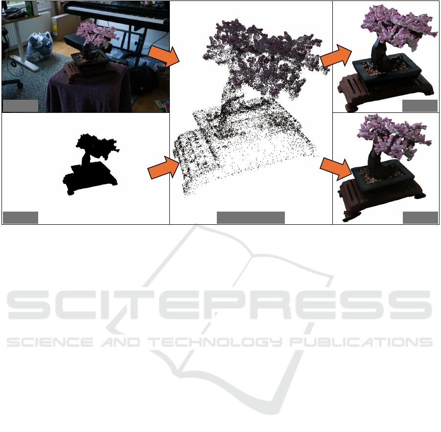
Figure 1: Our method, optimizes 2D Gaussians to accurately model specific object surfaces. They can be rendered directly or
exported as a mesh. For ease of viewing, the mask is inverted and the rendered image’s background is edited to be white.
ages from known poses. By optimizing the result-
ing rendered views to match the ground truth im-
ages, the MLP learns a 3D consistent geometry due to
the used volume rendering. Since then, many meth-
ods have further improved the quality of NeRF by
changing the sampling technique (Barron et al., 2021)
and enabling the use of unbounded scenes (Barron
et al., 2022). However, while these NeRFs are able
to produce high-quality novel views, they are pro-
hibitively expensive making real-time rendering im-
possible. Other works focus therefore on making
it possible to render NeRFs in real time by baking
the trained models into new representations (Hedman
et al., 2021; Reiser et al., 2023).
The introduction of 3DGS (Kerbl et al., 2023) of-
fers a new approach to tackle novel view synthesis
after NeRF. 3DGS does not rely on an MLP and in-
stead optimizes a discrete set of three-dimensional
Gaussians. Optimization is possible through a dif-
ferentiable rendering approach that utilizes tile-based
rasterization. It manages to achieve a quality that is
close to the best NeRF methods while being signifi-
cantly faster due to the efficient rendering approach.
This includes training the models faster and also real-
time rendering of the trained models. However, 3DGS
introduces a novel scene representation that cannot
be visualized or manipulated using traditional soft-
ware. Therefore, recent works try to expand the Gaus-
sian representation with additional features to support
e.g. relighting (Gao et al., 2023) and physics simula-
tions (Xie et al., 2023). Our method also uses a Gaus-
sian representation but offers support for traditional
software by enabling the extraction of a mesh.
2.2 Mesh Reconstruction
Traditional scene representations like meshes have
been around for a long time and benefit from strong
support in computer graphics applications. There-
fore, work has been published on converting the
previously mentioned representations into meshes.
One method modifies an underlying NeRF model to
better learn surfaces which are then baked into a
mesh (Yariv et al., 2023). The authors showcase var-
ious uses of their extracted meshes for downstream
tasks like physics simulation and appearance editing.
Other works, such as Neus (Wang et al., 2021) and
VolSDF (Yariv et al., 2021), directly optimize an im-
plicit signed distance function (SDF), which makes it
possible to obtain high-quality meshes. Finally, there
are also works that convert the explicit Gaussian rep-
resentations into meshes. SuGaR (Gu
´
edon and Lep-
etit, 2024) encourages 3D Gaussians to align them-
selves with surfaces in the scene, which can then be
used to extract a mesh.
Another approach is 2D Gaussian Splatting
(2DGS) (Huang et al., 2024), where the three-
dimensional Gaussians are replaced by two-
dimensional Gaussian discs. These Gaussian discs
are suited to model surfaces and are additionally
encouraged through regularization to gather closely
together to model surfaces of the scene. This ensures
ICPRAM 2025 - 14th International Conference on Pattern Recognition Applications and Methods
520

high-quality depth renders of the scene, which are
then used to extract a mesh. However, it is difficult
to create a mesh of a specific object in the scene
from the Gaussian representation that encompasses
the whole scene. This can only reliably be achieved
with the use of segmentation masks during the mesh
extraction. Using an available mask only during the
mesh creation is, however, wasteful because a lot of
computing power is used to reconstruct the entire
scene. Our method solves this by involving available
masks directly during the scene optimization. This
reduces compute resources and additionally makes
mesh generation easier by removing the need to
make assumptions about the scene bounds during the
extraction.
2.3 Object Reconstruction
The concurrent work GaussianObject (Yang et al.,
2024) also considers object-centric reconstruction.
However, their approach fundamentally differs from
ours. First, they consider very-sparse-view recon-
struction while we consider a standard multi-view re-
construction scenario. Although their approach han-
dles a more difficult scenario, they solve it through
special preprocessing and a multi-step training ap-
proach. The authors do not publish individual training
times but indicate an approximate time that is more
than three times slower than ours while using im-
ages at half the resolution. Second, they utilize 3D
Gaussians while we use 2D Gaussians. The 2D Gaus-
sian representation is better suited to extract meshes,
which improves the usability of our method for down-
stream applications (Huang et al., 2024).
3 PRELIMINARIES
3.1 Motivation
NeRF models tend to achieve very high accuracy
but are slow to train and render (Kerbl et al., 2023).
Follow-up works, such as SNeRG (Hedman et al.,
2021), convert NeRF models into representations that
are faster to render but the initial training step remains
slow. Gaussian models are fast to train and render im-
ages in real time while still producing excellent qual-
ity (Kerbl et al., 2023). However, the Gaussian rep-
resentation requires custom rendering software that
is not yet widely available. Additionally, modify-
ing the Gaussian representation or rendering pipeline,
such as is the case with 3DGS (Kerbl et al., 2023)
and 2DGS (Huang et al., 2024), requires correspond-
ing modifications in any downstream application that
supports Gaussians. The option to extract meshes en-
sures support for downstream tasks such as appear-
ance editing and physics simulations using existing
applications (Yariv et al., 2023). We will consider
2DGS as a foundation because they show fast train
and render times with high-quality rendering, as well
as the option to extract meshes from the underlying
representation.
3.2 2D Gaussian Splatting
We motivate our choice of 2DGS as the base for our
proposed method in Section 3.1, although our con-
tributions can be included in most Gaussian-based
methods. We validate this on the original 3DGS in
Appendix B. In the following, we will detail the gen-
eral steps of 2DGS, which will make the impact of
our contributions clearer. Figure 2 also provides an
overview including our proposed changes, which will
be discussed in Section 4. We refer to the 2DGS paper
as well as the previous 3DGS paper for more specifics
about the underlying principles.
3.2.1 Optimizing the Gaussian Representation
Given a set of n unstructured images I
i
∈ R
h×w×3
,
where i ∈ {1, ..., n} and h, w are the height and width
of the image, the goal is to create a geometrically ac-
curate 3D reconstruction that enables fast rendering of
novel views. In a preprocessing step, Structure from
Motion (SfM) is performed to obtain the SE(3) cam-
era poses P
i
∈ R
4×4
corresponding to each input im-
age I
i
. Additionally, SfM outputs a sparse point cloud
of the scene as a by-product of the pose estimation.
The sparse point cloud is used as a meaningful ini-
tialization by creating a 2D Gaussian for each point.
From here, the optimization loop starts: each itera-
tion, one of the input views I
i
is selected. Given the
input’s pose P
i
, a view R
i
∈ R
h×w×3
of the 2D Gaus-
sian representation is rendered. Then, a photometric
loss is computed between the rendered view R
i
and
the ground truth I
i
. Additionally, two regularization
terms are computed for the depths and normals of the
Gaussians used to render R
i
. Our proposed method
adds one additional loss term on the opacity of the
Gaussians as detailed in Section 4.2. Through back-
propagation, the position, shape, and appearance of
all involved Gaussians are updated to better fit the
color of I
i
. Lastly, there is an adaptive densification
control which duplicates and prunes Gaussians in set
intervals based on their accumulated gradients. We
propose to expand the adaptive densification control
with the pruning of occluded Gaussians which we de-
tail in Section 4.3. After optimizing for a set number
of iterations, all 2D Gaussians are exported as the 3D
Object-Centric 2D Gaussian Splatting: Background Removal and Occlusion-Aware Pruning for Compact Object Models
521

Render
Loss
SfM Points
2D Gaussians
Initialization
Camera
Projection
Adaptive
Density Control
Differentiable
Tile Rasterizer
Color
Depth
Normal
Alpha
Visibility
Tracking
Operation Flow Gradient Flow
2DGS
Ours
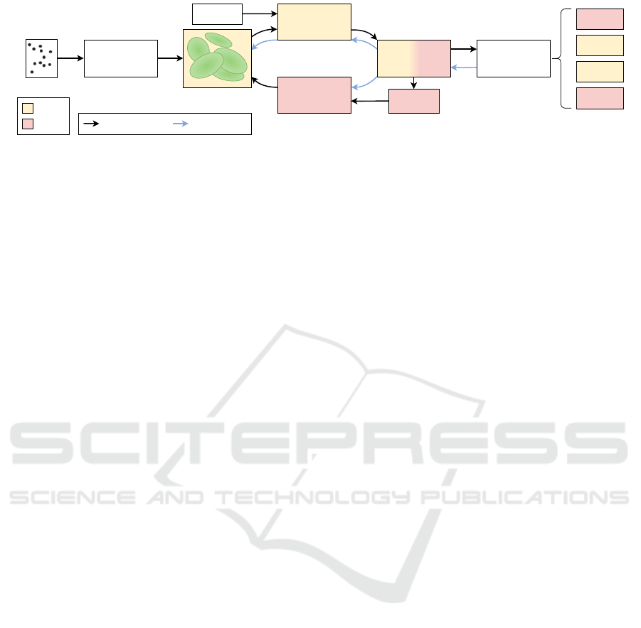
Figure 2: Overview of our method adapted from the 3DGS paper (Kerbl et al., 2023). Changes to the original pipeline are
highlighted for 2DGS and Ours. Overall, 2D Gaussians are initialized using a sparse SfM point cloud. During optimization,
the density of the Gaussians is adaptively controlled. The rasterization-based renderer enables very fast training and inference.
representation of the scene. While 2DGS optimizes
an entire scene, our proposed method learns a target
object and exports its isolated 3D representation (Sec-
tion 4).
3.2.2 Extracting Meshes
Optionally, it is possible to extract a mesh from the 2D
Gaussian representation. First, the scene is rendered
from each of the training poses P
i
, returning the col-
ors R
i
and depths D
i
∈ R
h×w×1
. From here, there are
two options: ’bounded’ and ’unbounded’ mesh ex-
traction. The bounded setting truncates the 3D repre-
sentation based on a depth value d
trunc
, which is ei-
ther empirically set or automatically estimated based
on the scene bounds. Using Open3d (Zhou et al.,
2018), a Truncated Signed Distance Function (TSDF)
volume is created from all R
i
and D
i
, where D
i
is
truncated based on d
trunc
. Finally, Open3D can con-
vert the TSDF volume into a triangle mesh. The un-
bounded setting instead considers the entire 3D rep-
resentation without any depth truncation by contract-
ing everything into a sphere. The authors then utilize
a customized TSDF computation and marching cube
algorithm to obtain a mesh.
2DGS optionally considers segmentation masks
M
i
∈ R
h×w×1
of an object O, with M
i
equals 1 for
pixels in I
i
that show O and M
i
equals 0 otherwise.
These segmentation masks are used during the mesh
extraction only if using the bounded setting. If M
i
is
available, before integration into the TSDF volume,
D
i
will additionally be truncated for pixels that do not
show O, i.e. M
i
equals 0. In Section 5.1, we will make
a distinction for 2DGS based on whether M
i
was used
to extract a mesh or not.
4 COMPACT OBJECT
RECONSTRUCTION
We use 2DGS as a base and expand it with our back-
ground loss (Section 4.2) and our pruning strategy for
occluded Gaussians (Section 4.3). Our background
loss utilizes segmentation masks M
i
to make the re-
construction object-centric, which reduces training
time and the size of the model. Our pruning strat-
egy removes unnecessary Gaussians, which reduces
the model size further without any loss in quality. Our
background loss requires masks M
i
, which are not al-
ways available. Section 4.1 details how we generate
masks if they are not available. An overview of the
method is shown in Figure 2, where contributions are
highlighted.
4.1 Mask Generation
Recent advances in image segmentation have made
the creation of object masks relatively easy. Using
Segment Anything 2 (SAM 2) (Ravi et al., 2024), it is
possible to semi-automatically generate masks of spe-
cific objects across an image sequence. Usually, it is
possible to generate accurate masks by interactively
setting only a few markers on an image. Objects seg-
mented in one image can then be propagated through
an entire image sequence. The accuracy is depen-
dent on the complexity of the image sequence and the
characteristics of the target object. If necessary, the
segmentation results can be refined by adding mark-
ers on additional images and propagating the new re-
sult. We utilize SAM 2 to generate object masks for
the scenes of the Mip-NeRF360 dataset (Barron et al.,
2022), which does not provide any masks. An exam-
ple mask is shown in Figure 3.
ICPRAM 2025 - 14th International Conference on Pattern Recognition Applications and Methods
522

4.2 Background Loss
2DGS is able to produce high-quality meshes of ob-
jects if segmentation masks are available. However,
the learned Gaussian representation consists of the
entire scene and the object is only isolated during
the mesh generation. This wastes computation re-
sources by reconstructing parts of the scene which
are discarded afterwards. Additionally, the underly-
ing Gaussians are not representative of the target ob-
ject. This makes them less suitable for applications
that are able to work directly with Gaussian represen-
tations because the object must first be isolated.
Our goal is to mask objects during the optimiza-
tion loop of 2DGS in order to reconstruct only the
necessary parts of the scene. Formally, given images
I
i
and corresponding segmentation masks M
i
of an ob-
ject O, let M
i
be 1 for pixels in I
i
where O is present
and 0 otherwise. When rendering the view R
i
, the ras-
terization of Gaussians should result in no Gaussians
where M
i
is 0. We formulate our background loss as
follows:
L
b
=
1
h ·w
∑
[A
i
·(1 −M
i
)], (1)
where A
i
∈ R
h×w×1
represents the accumulated al-
phas from Gaussians during rendering of R
i
. This is
highlighted in our pipeline as render loss on ’Alpha’
(Figure 2). Our background loss effectively penal-
izes Gaussian opacity where O is not present, pushing
them to become transparent. Transparent Gaussians
are automatically pruned via a threshold as part of the
3DGS density control.
The proposed background loss is, however, at
odds with the 3DGS photometric loss which pushes
the Gaussians to match the colors of R
i
and I
i
even
where M
i
is 0. To avoid training of unwanted parts
of the image, we multiply both I
i
and R
i
with M
i
to
compute the masked photometric loss L
M
c
.
L
M
c
(I
i
, R
i
, M
i
) = L
c
(I
i
·M
i
, R
i
·M
i
), (2)
Figure 3: Mask from SAM 2 overlaid on the input image.
where L
c
is the photometric loss from Equation 7 in
the 3DGS paper (Kerbl et al., 2023). We highlight this
in our pipeline as render loss on ’Color’ (Figure 2).
The total loss is as follows:
L = L
M
c
+ αL
d
+ βL
n
+ γL
b
, (3)
where L
d
is the 2DGS depth distortion loss and L
n
is
the 2DGS normal consistency loss. It is not necessary
to perform any masking on the two terms from 2DGS
since they do not influence the opacity of Gaussians.
4.3 Pruning Strategy
We introduce a novel pruning approach that tracks
which Gaussians have been used during rendering,
i.e., Gaussians that are involved in the alpha blend-
ing of any rendered pixel. We will refer to this con-
cept from here on as ’visible’ Gaussians or Gaussians
that are not ’occluded’. The concept is similar to the
’visibility filter’ used as part of the 3DGS density con-
trol, which tracks Gaussians that are inside the view-
ing frustum for a given view. However, there is a sig-
nificant difference between a Gaussian that is actually
visible and a Gaussian being in the field of view. For-
mally, given m Gaussians, let G
j
be a Gaussian that
is inside the viewing frustum and G
k
a Gaussian that
is outside the viewing frustum, where j, k ∈{1, ..., m}
and j ̸= k. During preprocessing, G
j
is projected to
the image and rasterized, identifying which pixels it
can contribute to. At the same time, G
k
is disqual-
ified from rendering and not assigned to any pixel.
During the rendering of a pixel p, all assigned Gaus-
sians are rendered in front-to-back order, accumulat-
ing their colors and opacities to p. Rendering is termi-
nated once either p reaches a threshold opacity close
to 1 or all assigned Gaussians have been exhausted.
Let us assume that all pixels that G
j
is assigned to,
reach the threshold opacity before reaching G
j
dur-
ing rendering. The 3DGS visibility filter will assign
G
j
with true and G
k
with false. We propose to assign
both G
j
and G
k
with false.
The motivation to track the visibility is clear:
Gaussians that are occluded cannot receive gradients
and no longer participate in the optimization process.
At the same time, these Gaussians are meaningless
to the overall scene representation since they exist in
a space that is not observed. A few Gaussians do
not occupy a lot of memory and require only a few
computations during preprocessing. However, with
scenes comprising millions of Gaussians, a substan-
tial amount of resources is wasted. We validate the
magnitude of occluded Gaussians in Section 5.3.2.
Object-Centric 2D Gaussian Splatting: Background Removal and Occlusion-Aware Pruning for Compact Object Models
523

5 EXPERIMENTS
We present evaluations of our proposed method and
its 2DGS baseline. For completeness, we also present
some results from previous state-of-the-art methods
that were compared with in the 2DGS paper (Huang
et al., 2024). Lastly, we will evaluate the efficacy of
each component of our method.
5.1 Implementation
We extend the custom CUDA kernels of 2DGS, which
are built upon the original 3DGS framework. Inside
the renderer, we save which Gaussians are used dur-
ing the color accumulation step. Regarding the adap-
tive density control, we use the same default values
as 2DGS, which correspond to the 3DGS defaults
at that time. The pruning of occluded Gaussians is
performed at an interval of 100 and 600 iterations
for the DTU (Jensen et al., 2014) and Mip-NeRF360
dataset (Barron et al., 2022), respectively. The loss
term coefficients as introduced by 3DGS and 2DGS
are unchanged. Although the inputs to the photomet-
ric loss are masked as described in Section 4.2. Our
background loss utilizes alpha maps returned from the
renderer. We set γ to 0.5 for the background loss in
all our experiments, unless stated otherwise. All ex-
periments on our method and 2DGS are run with 30k
iterations on an RTX3090 GPU.
Mesh Extraction. We use the 2DGS approach
detailed in Section 3.2 to extract meshes from the
learned Gaussian representation. Notably, we observe
that 2DGS uses masks during the extraction process
of the mesh. However, we believe this would be un-
fair when comparing with other methods that generate
meshes without using masks. For this reason, we will
consider our 2DGS results in two settings: 1) With
masks, and 2) Without masks. Where the first case
is equivalent to the standard 2DGS pipeline and in
the second case we skip the use of masks during the
mesh extraction. The use of masks to cull the final
mesh for the computation of the error metric is valid
in both scenarios. This is to isolate the error related
to the target object only. We will compare the results
of our proposed method and previous state-of-the-art
methods based on the use of masks accordingly. For
evaluations on the DTU dataset, we used the same val-
ues for voxel size and truncation thresholds as 2DGS
to enable a fair comparison. The only deviation is
given for our approaches with masks: we do not cull
the masks before computation of the error metric be-
cause our mesh already consists of only the target
object. Meshes generated from the Mip-NeRF360
dataset are only for qualitative comparison. There-
fore, we change the mesh extraction for our method
(with masks) to the unbounded mode with the voxel
size fixed to 0.004. Since our reconstructed scene
consists only of the object, we can safely turn the en-
tire scene into a mesh to obtain the object’s mesh. No-
tably, unlike the bounded setting, there is no need to
estimate any boundaries, making the unbounded set-
ting the most generalizable. Theoretically, it should
work for any object reconstruction using our proposed
method without the need to tweak any parameters.
5.2 Datasets
We evaluate our method on the DTU (Jensen et al.,
2014) and Mip-NeRF360 (Barron et al., 2022)
datasets. DTU consists of a subset of 15 scenes
from a larger dataset which are widely used for
evaluation by 3D reconstruction methods. Each of
the 15 scenes consists of either 49 or 64 images.
Point clouds obtained from a structured light scan-
ner serve as ground truth for 3D reconstructions. We
use the dataset provided by 2DGS, which already
combines the RGB images with object masks and
has the necessary sparse point cloud obtained from
Colmap (Sch
¨
onberger and Frahm, 2016; Sch
¨
onberger
et al., 2016) available. Additionally, we download the
ground truth point clouds from the DTU authors for
computation of the error metric. All experiments were
performed at the same 800 ×600 resolution as chosen
by the 2DGS authors.
Mip-NeRF360 consists of 9 scenes; 5 outdoor and
4 indoor. The outdoor and indoor scenes were cap-
tured with two cameras at resolutions of 4946 × 3286
and 3118 ×2078, respectively. Each scene consists of
between 125 and 311 images and a sparse point cloud
obtained from Colmap. All experiments on outdoor
scenes were performed at a resolution of 1237 × 822,
which roughly represents a downsampling by factor 4.
Experiments on the indoor scenes were performed at a
resolution of 1559 × 1039, which represents a down-
sampling by factor 2. These image resolutions are
the same as specified in the metric evaluation scripts
available from 3DGS and 2DGS.
5.3 Evaluations
5.3.1 DTU
We evaluate the quality of mesh reconstruction on the
DTU dataset using the chamfer distance. Here we
make a distinction between methods with masks and
methods without masks. In regards to 2DGS, we de-
tail this distinction in Section 5.1. Results from meth-
ods other than 2DGS and ours have been indicated
ICPRAM 2025 - 14th International Conference on Pattern Recognition Applications and Methods
524

Table 1: Quantitative comparison on the DTU dataset (Jensen et al., 2014) for methods with using masks. Results for methods
marked with † and ‡ are taken from the 2DGS (Huang et al., 2024) and Neus (Wang et al., 2021) papers, respectively. All
others are the results from our experiments. Time is indicated as hours or minutes. All others are chamfer distance. Green
indicates the best, yellow indicates the second-best, and orange indicates the third-best result.
w/ mask 24 37 40 55 63 65 69 83 97 105 106 110 114 118 122 Mean Time
impl.
NeRF
‡
1.83 2.39 1.79 0.66 1.79 1.44 1.50 1.20 1.96 1.27 1.44 2.61 1.04 1.13 0.99 1.54 N/A
Neus
‡
0.83 0.98 0.56 0.37 1.13 0.59 0.60 1.45 0.95 0.78 0.52 1.43 0.36 0.45 0.45 0.77 ∼14h
explicit
3DGS
†
2.14 1.53 2.08 1.68 3.49 2.21 1.43 2.07 2.22 1.75 1.79 2.55 1.53 1.52 1.50 1.96 11.2m
SuGaR
†
1.47 1.33 1.13 0.61 2.25 1.71 1.15 1.63 1.62 1.07 0.79 2.45 0.98 0.88 0.79 1.33 ∼1h
2DGS
†
0.48 0.91 0.39 0.39 1.01 0.83 0.81 1.36 1.27 0.76 0.70 1.40 0.40 0.76 0.52 0.80 10.9m
2DGS 0.45 0.82 0.31 0.38 0.95 0.83 0.80 1.30 1.16 0.68 0.66 1.36 0.39 0.66 0.48 0.75 10.94m
Ours 0.47 0.82 0.30 0.43 0.93 0.96 0.86 1.26 1.03 0.72 0.74 1.25 0.47 0.75 0.55 0.77 6.46m
Table 2: Quantitative comparison on the DTU dataset (Jensen et al., 2014) for methods without using masks. Results for
methods marked with † and ‡ are taken from the VolSDF (Yariv et al., 2021) and Neus (Wang et al., 2021) papers, respectively.
All others are the results from our experiments. Time is indicated as hours or minutes. All others are chamfer distance. Green
indicates the best, yellow indicates the second-best, and orange indicates the third-best result.
w/o mask 24 37 40 55 63 65 69 83 97 105 106 110 114 118 122 Mean Time
implicit
NeRF
‡
1.90 1.60 1.85 0.58 2.28 1.27 1.47 1.67 2.05 1.07 0.88 2.53 1.06 1.15 0.96 1.49 N/A
Neus
‡
1.00 1.37 0.93 0.43 1.10 0.65 0.57 1.48 1.09 0.83 0.52 1.20 0.35 0.49 0.54 0.84 ∼16h
VolSDF
†
1.14 1.26 0.81 0.49 1.25 0.70 0.72 1.29 1.18 0.70 0.66 1.08 0.42 0.61 0.55 0.86 ∼12h
expl.
2DGS 0.47 0.89 0.37 0.39 0.95 0.85 0.82 1.40 1.18 0.78 0.67 1.37 0.39 0.67 0.52 0.78 10.94m
Ours 0.49 0.88 0.37 0.39 1.01 0.83 0.82 1.41 1.27 0.76 0.71 1.28 0.41 0.66 0.54 0.79 10.76m
from which paper they have been taken. Our proposed
method, in the case of without masks, is equivalent to
only using the proposed pruning strategy Section 4.3.
The evaluation of quality and training time for the
case of with masks can be found in Table 1. We ob-
serve that our proposed method produces an equiva-
lent quality to the best implicit method Neus (Wang
et al., 2021) while being 100× faster. Compared to
the explicit methods, our method has a minor drop in
quality compared to 2DGS but is almost twice as fast.
We would also like to highlight that our method does
not require the mesh to be culled before the computa-
tion of the loss and indicates the quality of the entire
mesh. The discrepancy between the results reported
in the 2DGS paper and our own experiments is due
to improvements to the code that the authors have re-
leased since the publication of their paper.
The evaluation of quality and training time for the
case without using masks can be found in Table 2.
We observe that there is almost no difference in qual-
ity between our proposed method and 2DGS. This is
because our pruning strategy removes only unneces-
sary Gaussians. At the same time, the reduced num-
ber of Gaussians positively impacts the speed of our
method, making it a little faster. We would like to note
that the gain in speed is not that significant due to the
occluded Gaussians not taking part in the rendering
itself. For this reason, we will also evaluate the num-
ber of Gaussians separately. Compared to the implicit
methods, both our proposed method and 2DGS pro-
duce higher-quality meshes while being significantly
faster.
Table 3 gives an overview of the performance of
Table 3: Performance comparison on the DTU dataset.
Methods marked with ⋆ are without using masks.
CD↓ Time↓ Gaussians↓ Storage↓
2DGS
⋆
0.782 10.94 min 198,820 46.21 MB
Ours
⋆
0.787 10.76 min 178,332 41.45 MB
2DGS 0.748 10.94 min 198,820 46.21 MB
Ours 0.769 6.46 min 108,568 25.23 MB
our proposed method and 2DGS in two settings: with
and without using masks. In the without mask case,
our method produces an almost identical quality while
reducing the final number of Gaussians by about 10%
on average. This positively impacts the training time
but most significantly reduces memory requirements
and the storage size of the exported model. The
underlying representation of 2DGS does not change
between the with and without mask scenario, only
the output mesh. For this reason, the training time
and number of Gaussians are the same. Our method
with masks halves the number of Gaussians over the
2DGS. This improves the training time more signifi-
cantly and the exported model is roughly half as large.
Although there is a minor drop in quality compared to
2DGS, it is still exceptional compared to the state of
the art shown previously.
5.3.2 Mip-NeRF360
The Mip-NeRF360 dataset does not have a ground
truth geometry, which makes quantitative evaluation
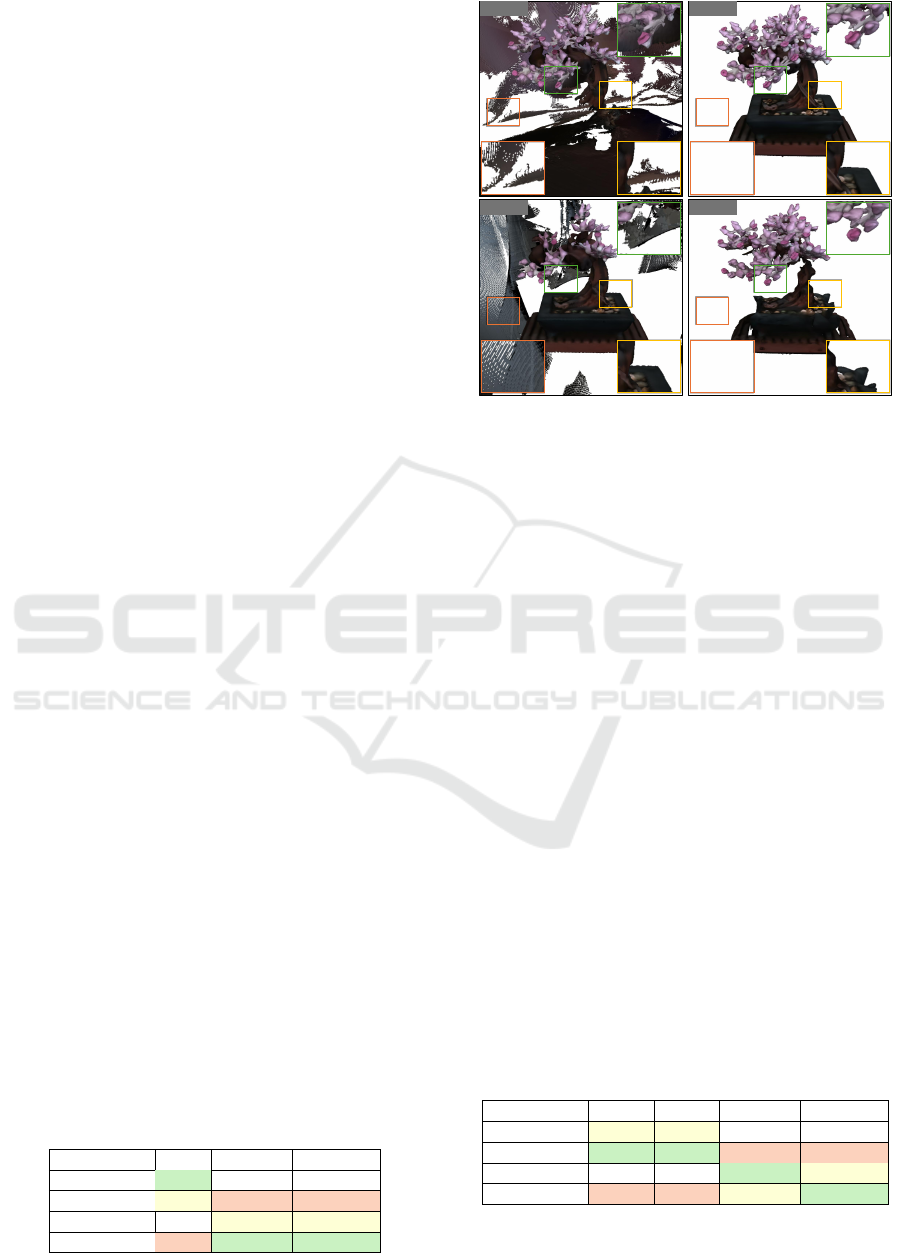
only possible for novel view rendering. A qualitative
comparison of the meshes is shown in Figure 4. We
evaluate the quality of novel view rendering using the
peak signal-to-noise ratio (PSNR) and the structural
Object-Centric 2D Gaussian Splatting: Background Removal and Occlusion-Aware Pruning for Compact Object Models
525

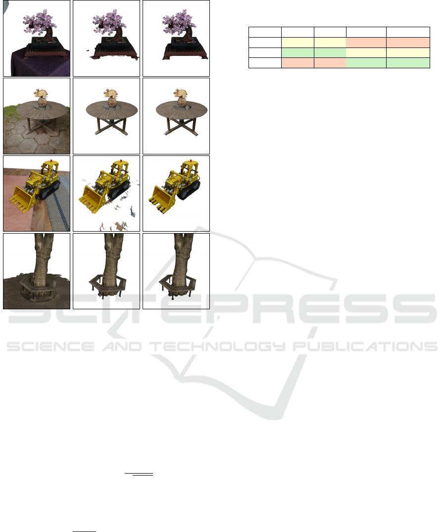
(a) 2DGS (b) 2DGS +
Our Masks
(c) Ours
Figure 4: Qualitative comparison of rendered meshes on
the Mip-NeRF360 dataset. 2DGS meshes are extracted
as bounded mesh with automatically estimated parameters.
Ours is the full model extracted as unbounded mesh.
similarity index measure (SSIM) between the ground
truth and rendered images. Because our method re-
constructs only the necessary parts of the scene, we
consider only a masked PSNR and SSIM in all our
evaluations. The masked PSNR is given by the fol-
lowing equation:
PSNR = 20 log
10
(
MAX
I
√
MSE
), (4)
where MAX
I
represents the maximum possible inten-
sity and MSE represents the masked MSE as follows.
MSE =
1
∑
(M)
∑
[(GT −R
c
) ·M]
2
(5)
Masking the SSIM is not straightforward because it
uses windows. We choose to apply the mask to the
ground truth and rendered image before computing
the SSIM. In the last step, we compute the mean only
over the valid pixels. We want to note that this will
cause invalid pixels to be within the windows of some
Table 4: Performance comparison on the Mip-NeRF360
dataset. Methods marked with ⋆ are without using masks.
PSNR↑ SSIM↑ Time↓ Gaussians↓
2DGS
⋆
28.31 0.875 31.44 min 2,053,425
Ours
⋆
28.35 0.876 31.28 min 1,875,546
Ours 25.69 0.822 9.15 min 73,179
valid pixels, which will influence the score. The in-
fluence would be slightly positive due to the pixels
outside of the mask being identical due to masking
the inputs.
The quantitative evaluation on the Mip-NeRF360
dataset can be found in Table 4. Please note that the
difference between 2DGS with and without masks oc-
curs only during the mesh extraction. Because we
evaluate the views rendered from the Gaussian rep-
resentation directly, they are equivalent. We notice
that there is no significant impact on quality from our
method without masks. However, we are able to re-
move almost 10% of Gaussians ’for free’, which pos-
itively impacts training time and the storage size of
the exported model. In the case of with masks, our
method reduces the number of Gaussians by over 95%
and reduces training times by 70%. Compared to the
DTU dataset, the Mip-NeRF scenes are much larger
and more complex. The size and complexity of a
scene directly influence the number of Gaussians that
are necessary to accurately model it. By using masks
to focus on a specific object, we are able to discard a
lot of unnecessary scene modeling. Although there is
a small decrease in quality, we note that some errors in
individual masks can cause the comparison to be bi-
ased against our method. Figure 5 shows an example
of an erroneous mask that includes non-object pix-
els. This negatively influences the evaluation of our
method that only reconstructs the target object, while
not affecting the baseline that reconstructs the entire
scene. However, this also shows that our method is
robust to minor errors in individual masks. Figure 6
shows an example rendering from our method of the
same view. The erroneously masked part of the im-
age is not part of the reconstruction, while the parts of
the object that are missing in the mask are correctly
reconstructed.
We additionally evaluate the magnitude of oc-
cluded Gaussians by loading trained Gaussian rep-
resentations and rendering all training views while
tracking the Gaussian visibility. A visualization of
occluded Gaussians for 2DGS is shown in Figure 7.
The results for the Mip-NeRF360 dataset are shown
in Table 5. We observe that on average as many as
10% of Gaussians in outdoor scenes are occluded. For
indoor scenes, there are on average still close to 3%
of Gaussians occluded. Using our pruning approach,
we are able to significantly reduce the number of oc-
ICPRAM 2025 - 14th International Conference on Pattern Recognition Applications and Methods
526

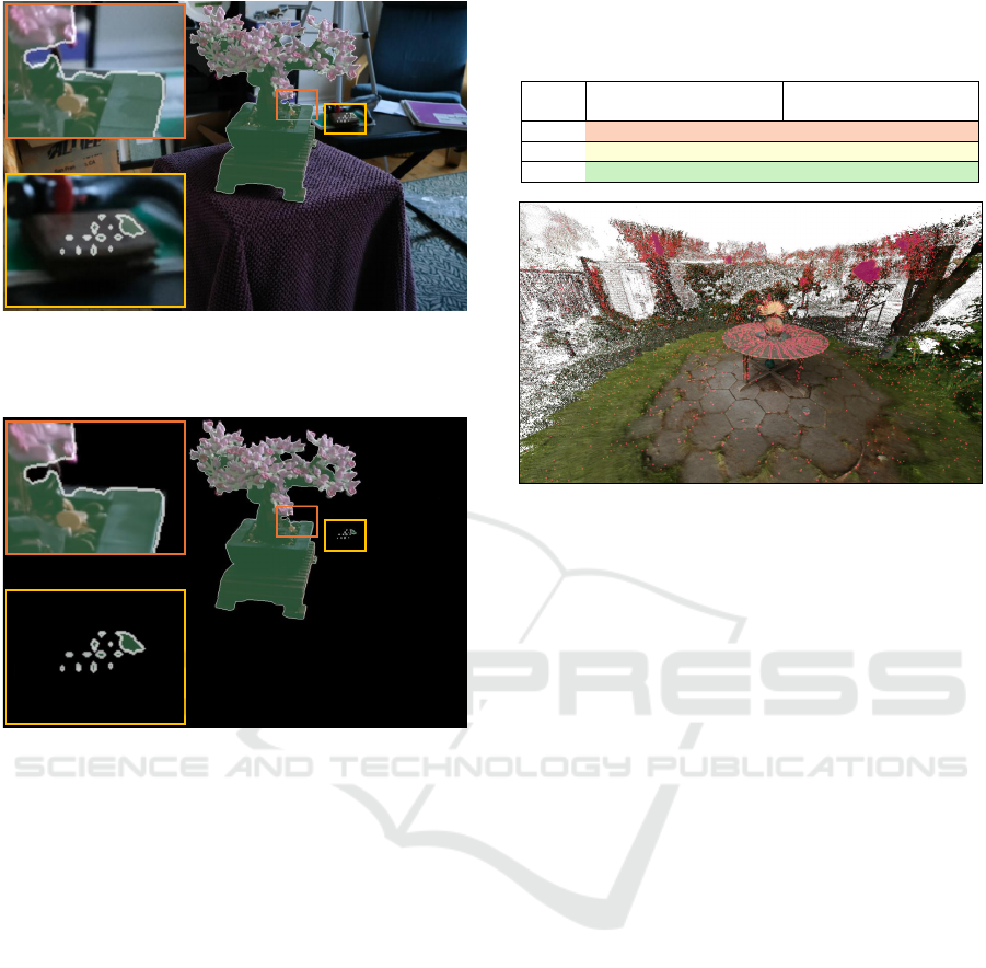
Figure 5: Example of erroneous mask overlaid on the input
image. Yellow box: non-object pixels are in mask. Orange
box: some object pixels are outside mask.
Figure 6: Example rendering overlaid with the correspond-
ing mask. Yellow box: non-object pixels in mask are not
reconstructed. Orange box: object pixels missing in mask
are still reconstructed.
cluded Gaussians to below 1%. In the case of our full
method including object masking, the contribution of
occluded Gaussians is further reduced to below 0.3%.
We would like to note that the reason for any occluded
Gaussians remaining in our proposed method are due
to the adaptive density control being suspended in the
second half of the training. At that point, it is still
possible for Gaussians to be occluded from all views.
However, if we continued pruning, any pruning of e.g.
temporarily occluded Gaussians could no longer be
fixed by densification. If it is desired to remove all
occluded Gaussians from the final representation, it is
also possible to prune them in an additional step after
optimization is finished. This can be done in the same
way as we computed the number of occluded Gaus-
sians for this evaluation, followed by the removal of
those Gaussians before exporting the final representa-
tion.
Table 5: Evaluation of occluded Gaussians on the Mip-
NeRF360 dataset. Methods marked with ⋆ are without us-
ing masks.
Outdoor Scenes Indoor Scenes
Occluded↓ Occluded/Total↓ Occluded↓ Occluded/Total↓
2DGS
⋆
328088 9.81% 19333 2.65%
Ours
⋆
25888 1.00% 3456 0.49%
Ours 358 0.26% 31 0.09%
Figure 7: Visualization of occluded Gaussians for 2DGS
overlaid on the Garden scene from the Mip-NeRF360
dataset. Red areas highlight locations of occluded Gaus-
sians.
5.4 Ablation
We evaluate the design choices of our proposed
method. To begin, we will show the effectiveness of
each component as chosen by us. Afterward, we will
consider the components individually and reason the
choices.
5.4.1 Full Model
Table 6 and Table 7 show that our pruning strategy
alone (B) reduces the number of Gaussians and train-
ing time without impacting the quality in a meaning-
ful way. It arguably is a ’free’ reduction of model
size and gives a small speed up. At the same time,
our masking approach alone (C) reduces the train-
ing time and the number of Gaussians more signif-
icantly. However, this comes at a small loss in ac-
curacy. Overall, our proposed method (D) is able to
significantly reduce the training time and number of
Gaussians with only a small reduction in quality. The
loss in quality is at least partially due to masking er-
rors as discussed in Section 5.3.2 and showcased in
Figure 6.
5.4.2 Pruning
We show the motivation for our pruning strategy
in Section 5.3.2: On average between 2.65% and
9.81% of all Gaussians are not visible for the baseline
method. Our pruning strategy is able to reduce the
Object-Centric 2D Gaussian Splatting: Background Removal and Occlusion-Aware Pruning for Compact Object Models
527

number of total Gaussians as has been shown through-
out all experiments. Removed Gaussians representing
occluded ones are signified by Table 5, which shows
that using our pruning strategy, the number of oc-
cluded Gaussians in the final representation is on av-
erage reduced by 80% to 90%.
5.4.3 Background Loss
We justify our masking approach of the background
to enable object-centric reconstruction. Figure 8
shows a comparison of different masking approaches.
When masking only the photometric loss, the geom-
etry breaks and Gaussians remain in the background
causing noise. Using only the background loss with
a small lambda results in better geometry but Gaus-
sians remain in the background, causing noise as in
the previous case. Increasing the lambda of the back-
ground loss will eventually result in the removal of
all background Gaussians, however, the geometry suf-
fers. The reason for this can be twofold. First, is the
case of occlusions, where the object is occluded by
another object. Second, is the case of an erroneous
mask, where pixels belonging to the object are incor-
rectly marked as not being part of the object (Fig-
ure 5). In both cases, the mask will penalize Gaus-
sians that are correctly representing our object be-
cause the mask will indicate that the object is not vis-
ible. Due to the larger lambda, which is necessary
to remove all background Gaussians, the penalized
Gaussians would be influenced too strongly. Our pro-
posed masking approach is able to properly remove
background Gaussians while keeping the object’s ge-
ometry intact.
5.5 Limitations
Our proposed method works well for the reconstruc-
tion of a range of objects but has limitations. First, our
method inherits limitations specific to 2DGS, such as
a difficulty to handle semi-transparent surfaces. Sec-
ond, our proposed background loss depends on the
quality of the input masks. While it is robust to some
errors in individual masks, systematic errors will re-
sult in bad reconstructions. Additionally, the genera-
tion of masks itself is highly dependent on the char-
acteristics of the object and the scene it is located in.
Table 6: Ablation studies comparing the influence of each
of our proposed components on the DTU dataset.
CD↓ Time↓ Gaussians↓
A. baseline 0.748 10.94 min 198,820
B. w/ pruning 0.750 10.76 min 178,332
C. w/ masking 0.772 7.17 min 136,561
D. Full Model 0.769 6.46 min 108,568
Photometric
Loss
Both
(Ours)
Background
Loss
Background
Loss (large λ)
Figure 8: Ablation studies for background removal. Shown
is masking of the photometric loss only, using our back-
ground loss only, using our background loss only with a
large coefficient, and our proposed masking approach.
We show an example of failure cases in Appendix C.
In the future, better methods for the generation of seg-
mentation masks will alleviate this problem.
6 CONCLUSIONS
We propose an object reconstruction approach utiliz-
ing 2D Gaussians. Our method utilizes a novel back-
ground loss with guidance from segmentation masks.
We are able to accurately reconstruct object surfaces
even in cases of erroneous masks. Additionally, we
propose a pruning approach that removes occluded
Gaussians during training, reducing the size of the
model without impacting quality. The object-centric
reconstruction enables direct use of the learned model
in downstream applications (Appendix A). Lastly, the
2D Gaussian representation is well suited for con-
version to meshes. This enables support for applica-
tions that do not support the Gaussian representation,
such as appearance editing and physics simulation for
meshes.
Table 7: Ablation studies comparing the influence of each
of our proposed components on the Mip-NeRF360 dataset.
PSNR↑ SSIM↑ Time↓ Gaussians↓
A. baseline 28.31 0.875 31.44 min 2,053,425
B. w/ pruning 28.35 0.876 31.28 min 1,875,546
C. w/ masking 25.66 0.821 9.12 min 74,477
D. Full Model 25.69 0.822 9.15 min 73,179
ICPRAM 2025 - 14th International Conference on Pattern Recognition Applications and Methods
528

ACKNOWLEDGEMENTS
This work was co-funded by the European Union
under Horizon Europe, grant number 101092889,
project SHARESPACE. We thank Ren
´
e Schuster
for constructive discussions and feedback on earlier
drafts of this paper.
REFERENCES
Barron, J. T., Mildenhall, B., Tancik, M., Hedman, P.,
Martin-Brualla, R., and Srinivasan, P. P. (2021). Mip-
nerf: A multiscale representation for anti-aliasing
neural radiance fields. ICCV.
Barron, J. T., Mildenhall, B., Verbin, D., Srinivasan, P. P.,
and Hedman, P. (2022). Mip-nerf 360: Unbounded
anti-aliased neural radiance fields. CVPR.
Gao, J., Gu, C., Lin, Y., Zhu, H., Cao, X., Zhang, L., and
Yao, Y. (2023). Relightable 3d gaussian: Real-time
point cloud relighting with brdf decomposition and
ray tracing. arXiv:2311.16043.
Gu
´
edon, A. and Lepetit, V. (2024). Sugar: Surface-aligned
gaussian splatting for efficient 3d mesh reconstruction
and high-quality mesh rendering. CVPR.
Hedman, P., Srinivasan, P. P., Mildenhall, B., Barron, J. T.,
and Debevec, P. (2021). Baking neural radiance fields
for real-time view synthesis. ICCV.
Huang, B., Yu, Z., Chen, A., Geiger, A., and Gao, S. (2024).
2d gaussian splatting for geometrically accurate radi-
ance fields. In SIGGRAPH 2024 Conference Papers.
Association for Computing Machinery.
Jensen, R., Dahl, A., Vogiatzis, G., Tola, E., and Aanæs,
H. (2014). Large scale multi-view stereopsis evalua-
tion. In 2014 IEEE Conference on Computer Vision
and Pattern Recognition, pages 406–413. IEEE.
Kerbl, B., Kopanas, G., Leimk
¨
uhler, T., and Drettakis,
G. (2023). 3d gaussian splatting for real-time radi-
ance field rendering. ACM Transactions on Graphics,
42(4).
Mildenhall, B., Srinivasan, P. P., Tancik, M., Barron, J. T.,
Ramamoorthi, R., and Ng, R. (2020). Nerf: Repre-
senting scenes as neural radiance fields for view syn-
thesis. In ECCV.
Ravi, N., Gabeur, V., Hu, Y.-T., Hu, R., Ryali, C., Ma,
T., Khedr, H., R
¨
adle, R., Rolland, C., Gustafson, L.,
Mintun, E., Pan, J., Alwala, K. V., Carion, N., Wu,
C.-Y., Girshick, R., Doll
´
ar, P., and Feichtenhofer, C.
(2024). Sam 2: Segment anything in images and
videos. arXiv preprint arXiv:2408.00714.
Reiser, C., Szeliski, R., Verbin, D., Srinivasan, P. P.,
Mildenhall, B., Geiger, A., Barron, J. T., and Hedman,
P. (2023). Merf: Memory-efficient radiance fields for
real-time view synthesis in unbounded scenes. SIG-
GRAPH.
Sch
¨
onberger, J. L. and Frahm, J.-M. (2016). Structure-
from-motion revisited. In Conference on Computer
Vision and Pattern Recognition (CVPR).
Sch
¨
onberger, J. L., Zheng, E., Pollefeys, M., and Frahm, J.-
M. (2016). Pixelwise view selection for unstructured
multi-view stereo. In European Conference on Com-
puter Vision (ECCV).
Wang, P., Liu, L., Liu, Y., Theobalt, C., Komura, T., and
Wang, W. (2021). Neus: Learning neural implicit sur-
faces by volume rendering for multi-view reconstruc-
tion. NeurIPS.
Xie, T., Zong, Z., Qiu, Y., Li, X., Feng, Y., Yang, Y., and
Jiang, C. (2023). Physgaussian: Physics-integrated
3d gaussians for generative dynamics. arXiv preprint
arXiv:2311.12198.
Yang, C., Li, S., Fang, J., Liang, R., Xie, L., Zhang, X.,
Shen, W., and Tian, Q. (2024). Gaussianobject: High-
quality 3d object reconstruction from four views with
gaussian splatting. ACM Transactions on Graphics,
43(6).
Yariv, L., Gu, J., Kasten, Y., and Lipman, Y. (2021). Vol-
ume rendering of neural implicit surfaces. In Thirty-
Fifth Conference on Neural Information Processing
Systems.
Yariv, L., Hedman, P., Reiser, C., Verbin, D., Srinivasan,
P. P., Szeliski, R., Barron, J. T., and Mildenhall, B.
(2023). Bakedsdf: Meshing neural sdfs for real-time
view synthesis. arXiv.
Zhou, Q.-Y., Park, J., and Koltun, V. (2018). Open3D:
A modern library for 3D data processing.
arXiv:1801.09847.
APPENDIX
Downstream Applications
Our method produces an isolated representation of a
target object from the scene. Whether using Gaus-
sians or mesh, the representation can be directly used
without any need for additional processing. This en-
ables quick and easy use for downstream applications,
such as appearance editing and physics simulations.
An example of appearance editing is shown in Fig-
ure 9.
Pruning in 3D Gaussian Splatting
We demonstrate the versatility of our pruning strat-
egy by implementing it in 3DGS. We perform a sin-
gle experiment on the Bicycle scene from the Mip-
NeRF360 dataset as proof of principle. The results
are shown in Table 8. Similar to the results for 2DGS,
our pruning strategy effectively reduces the number
of occluded Gaussians while preserving quality. This
reduces memory requirements and positively impacts
the training time. However, we notice that the num-
ber of occluded Gaussians is lower compared to the
2DGS scenes. This is likely due to 2DGS encourag-
ing surfaces that are fully opaque. The result is a clear
Object-Centric 2D Gaussian Splatting: Background Removal and Occlusion-Aware Pruning for Compact Object Models
529

(a) Mesh (b) Gaussians
Figure 9: Appearance editing on the Mip-NeRF360 dataset
by combining the Treehill and Bonsai scenes.
Table 8: Evaluation of our pruning strategy in 3DGS. Re-
sults on the Bicycle scene from the Mip-NeRF360 dataset.
PSNR↑ Time↓ Gaussians↓ Occluded↓ Occluded%↓
3DGS 25.23 33.1 min 4,945,971 114,286 2.31%
Pruning 25.29 32.8 min 4,830,703 9,793 0.20%
boundary of Gaussians that are visible and Gaussians
that are occluded. In the case of 3DGS, Gaussians can
be spread out along viewing rays, which can result in
semi-transparent surfaces. This allows for Gaussians
to stay visible across different viewing angles. De-
spite the reduced magnitude of occluded Gaussians in
3DGS, we show that our pruning strategy provides a
’free’ boost to the performance.
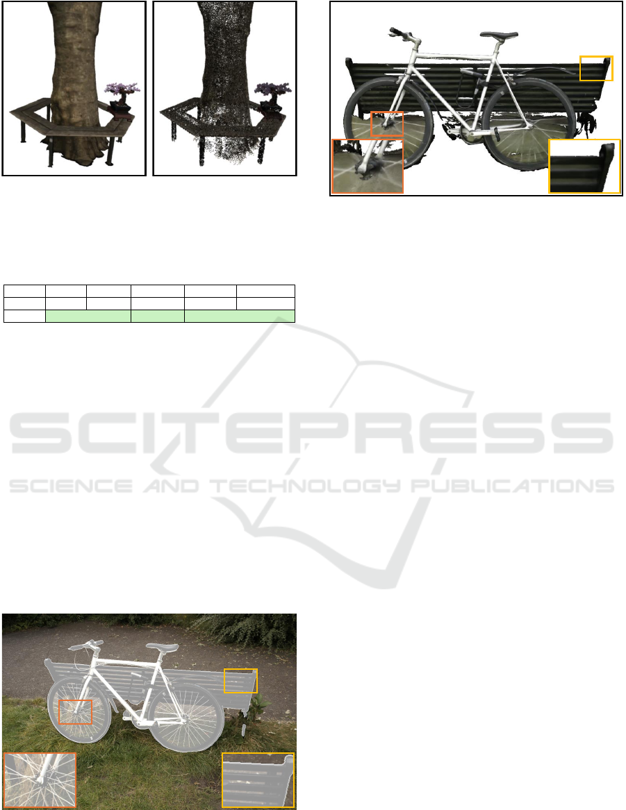
Failure Cases
The mask generation using SAM 2 is easy and fast but
the quality depends on the characteristics of the target
object. We highlight a failure case with thin structures
in the Bicycle scene of the Mip-NeRF360 dataset in
Figure 10. This is a consistent error that propagates
Figure 10: Example failure case for mask generation using
SAM 2. Gaps in the bench and between the bicycle spokes
are included.
Figure 11: Example failure case for our method with con-
sistent errors in masks. Gaps in the bench and between the
bicycle spokes are used to model the background.
through all views of the dataset. The errors cause our
method to learn an incorrect representation as shown
in Figure 11. Due to the masks, our method consid-
ers the gaps as part of the object, which results in a
surface. The color represents an average of the back-
ground that is visible through the gaps. However, we
note that our method is robust against some masking
errors in individual views as shown in Figure 6.
ICPRAM 2025 - 14th International Conference on Pattern Recognition Applications and Methods
530