Improving Adaptive Density Control for 3D Gaussian Splatting
Glenn Grubert
1,2,∗ a
, Florian Barthel
1,2,∗ b
, Anna Hilsmann
2 c
and Peter Eisert
1,2 d
1
Humboldt Universit
¨
at zu Berlin, Berlin, Germany
2
Fraunhofer HHI, Berlin, Germany
Keywords:
Gaussian Splatting, Adaptive Density Control, Densification, Novel View Synthesis, 3D Scene
Reconstruction.
Abstract:
3D Gaussian Splatting (3DGS) has become one of the most influential works in the past year. Due to its
efficient and high-quality novel view synthesis capabilities, it has been widely adopted in many research
fields and applications. Nevertheless, 3DGS still faces challenges to properly manage the number of Gaussian
primitives that are used during scene reconstruction. Following the adaptive density control (ADC) mechanism
of 3D Gaussian Splatting, new Gaussians in under-reconstructed regions are created, while Gaussians that do
not contribute to the rendering quality are pruned. We observe that those criteria for densifying and pruning
Gaussians can sometimes lead to worse rendering by introducing artifacts. We especially observe under-
reconstructed background or overfitted foreground regions. To encounter both problems, we propose three
new improvements to the adaptive density control mechanism. Those include a correction for the scene extent
calculation that does not only rely on camera positions, an exponentially ascending gradient threshold to
improve training convergence, and significance-aware pruning strategy to avoid background artifacts. With
these adaptions, we show that the rendering quality improves while using the same number of Gaussians
primitives. Furthermore, with our improvements, the training converges considerably faster, allowing for
more than twice as fast training times while yielding better quality than 3DGS. Finally, our contributions are
easily compatible with most existing derivative works of 3DGS making them relevant for future works.
1 INTRODUCTION
In the past year, 3D Gaussian Splatting (3DGS)
(Kerbl et al., 2023) has emerged as a powerful tool for
real-time 3D scene reconstruction. By representing a
scene with a large collection of 3D Gaussian primi-
tives (or splats), each being described by a position, a
color, a density, a scale and a rotation, 3DGS is able
to model complex structures with high fidelity while
allowing very fast rendering.
Although rendering using splats has been around
for many years (Zwicker et al., 2001; Botsch et al.,
2005; Pfister et al., 2000; Ren et al., 2002), 3DGS,
for the first time, allows differential rendering. This
makes the method applicable for a large range of re-
search fields, such as gradient-based novel-view syn-
thesis, generative models, style transfer, scene edit-
a
https://orcid.org/0009-0007-9423-7533
b
https://orcid.org/0009-0004-7264-1672
c
https://orcid.org/0000-0002-2086-0951
d
https://orcid.org/0000-0001-8378-4805
∗
Equal contributions.
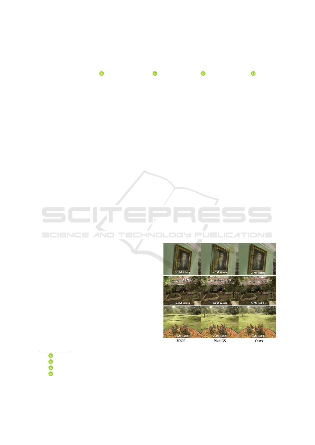
Figure 1: Rendered novel views from the drjohnson, garden
and flowers scene using 3DGS, PixelGS and our method.
Our method produces better backgrounds, creates less arti-
facts and uses the same number of Gaussians as 3DGS.
ing, animation, and many other (Luiten et al., 2024;
610
Grubert, G., Barthel, F., Hilsmann, A. and Eisert, P.
Improving Adaptive Density Control for 3D Gaussian Splatting.
DOI: 10.5220/0013308500003912
Paper published under CC license (CC BY-NC-ND 4.0)
In Proceedings of the 20th International Joint Conference on Computer Vision, Imaging and Computer Graphics Theory and Applications (VISIGRAPP 2025) - Volume 2: VISAPP, pages
610-621
ISBN: 978-989-758-728-3; ISSN: 2184-4321
Proceedings Copyright © 2025 by SCITEPRESS – Science and Technology Publications, Lda.

Liu et al., 2024; Barthel et al., 2024; Bagdasarian
et al., 2024). In its main application, the novel view
synthesis, a 3D scene is generated from multiple 2D
views of a target environment along with their respec-
tive camera positions. Specifically, with the differen-
tiable rendering property of 3DGS, a loss between a
rendered view and a target view can be computed, and
the Gaussian attributes in the scene are updated via
gradient descent. This is done until the optimization
converges and a resulting 3D scene is constructed,
which can be viewed from arbitrary novel views. Be-
fore, this was achieved mainly using neural radiance
field methods, e.g. NeRF, Mip-NeRF, Instant NGP
or Plenoxels (Mildenhall et al., 2020; Barron et al.,
2021; Fridovich-Keil and Yu et al., 2022; M
¨
uller
et al., 2022). Although NeRF-based approaches pro-
duce very high rendering quality for novel views, they
are slow to train and slow to render. This is because
they have to query a small neural network multiple
times to render a single pixel. Additionally, NeRFs
store a 3D scene implicitly in the weights of a neural
network, making it difficult to incorporate them into
explicit 3D environments, such as game engines or
virtual reality settings. 3DGS, in contrast, represents
the scene with explicit 3D Gaussian splats, enabling a
smooth integration into explicit 3D environments.
Despite its success, 3DGS encounters certain lim-
itations. One major challenge lies in managing in
the number of Gaussian primitives and their distri-
bution within . scene For example, in coarse and
smooth regions, a small number of large Gaussians
can be sufficient, whereas regions with fine and com-
plex structures require a large number of small Gaus-
sians. 3DGS addresses this through an adaptive den-
sity control (ADC) mechanism, where the Gaussians
are cloned or split .if their associated position changes
frequently during optimization and deleted if their
opacity drops below a certain threshold. Although the
ADC algorithm of 3DGS already yields high-quality
results in many cases, it tends to generate too many
Gaussians in simple regions, leading to overfitting
and, conversely, under-reconstructs highly complex
regions, such as grass. In this paper, we propose an
improved ADC algorithm designed to enhance recon-
struction quality while reducing the number of Gaus-
sian primitives required, surpassing the efficiency of
state-of-the-art methods through the following contri-
butions:
1. Exponential Gradient Thresholding: We intro-
duce an exponentially ascending gradient thresh-
old that accelerates convergence and improves
stability during optimization, particularly in com-
plex regions.
2. Corrected Scene Extent for Adaptive Cloning
and Splitting: By adjusting the scene extent cal-
culation to account for view depth, our approach
ensures a more accurate distribution of Gaussians,
optimizing both dense and sparse regions.
3. Significance-Aware Pruning: Our novel pruning
criterion evaluates the impact of each Gaussian on
overall scene fidelity, reducing unnecessary primi-
tives while preserving high reconstruction quality.
In the following sections, we will first provide a
detailed overview of 3DGS and its ADC algorithm
(section 2). We then discuss related work on the ADC
algorithm of Gaussian Splatting (section 3). Section
4 describes our proposed method, followed by exper-
iments and an ablation study (section 5) and a conclu-
sion (section 6).
2 PRELIMINARIES
2.1 Gaussian Primitives
3D Gaussian splatting uses 3D Gaussian distributions
F : R
3
→ R
+
to represent a scene (Kerbl et al., 2023).
A 3D Gaussian function is parameterized by a (3×3)
covariance matrix Σ and a 3D mean vector µ. Σ de-
scribes the extent of a Gaussian function in 3D space,
while µ characterizes its position or center (Zwicker
et al., 2001). The covariance Σ can be parameterized
by a 4D quaternion vector q, describing the rotation,
and a 3D scaling vector s. The kernel K of a multivari-
ate Gaussian distribution is defined as follows (Bul
`
o
et al., 2024):
K[µ, Σ](x) = exp

−
1
2
(x − µ)
⊤
Σ
−1
(x − µ)

(1)
To obtain a Gaussian primitive, a 3D Gaussian
function is extended by two additional attributes: an
opacity value o and a feature vector c. The opacity de-
scribes how transparent a primitive is displayed, and c
modulates the color in which a primitive is displayed
(Kerbl et al., 2023).
For simplicity, from now on these primitives will
be referred to as Gaussians. Thus, a Gaussian g
k
can
be described as a 4-tuple (µ
k
, Σ
k
, o
k
, c
k
). A 3D Gaus-
sian model scene representation G can be described
as a set of n Gaussians {g
1
, . . . , g
n
}.
2.2 Alpha Blending
The first step towards rendering is to select only those
Gaussians Ω ⊆ G that appear within the camera view.
For rendering, these 3D Gaussians are projected
onto the 2D image plane of a selected view. The ob-
tained 2D Gaussians g
′
k
= (µ
′
k
, Σ
′
k
, o
k
, c
k
), from now on
Improving Adaptive Density Control for 3D Gaussian Splatting
611

referred to as splats, then contribute to the color of the
pixels they cover on that plane (Kerbl et al., 2023). µ
′
k
and Σ
′
k
are the view-dependent parameterizations of
the 2D projection, and o
k
is the opacity, while c
k
is
the feature vector inherited from g
k
.
Let L = (g
′
1
, . . . , g
′
m
) be a list of ascending depth-
sorted splats that cover a pixel p. K[µ, Σ] denotes a
Gaussian kernel defined in Equation 1. Alpha blend-
ing can then be described as follows (Bul
`
o et al.,
2024):
color
p
=
m
∑
k=1
c
k
·
w
k
z}|{
α
k
·t
k
(2)
α
k
= o
k
· K[µ
′
k
, Σ
′
k
](p) (3)
t
k
=
k−1
∏
j=1
(1 − α
j
) (4)
Equation 2 iterates over all m splats in the list and
computes the final RGB color
p
for a pixel p. There-
fore, the color c
k
and the alpha-blending coefficient
w
k
are multiplied per splat. w
k
weights the color con-
tribution of a splat to a pixel. Equation 3 computes
the alpha value for a splat, given a pixel p. The com-
putation of w
k
considers the opacity and density of
a given splat (transparency α
k
) and of all its prede-
cessors (transmittance t
k
, Eq. 4). Thus, the frontmost
splat’s color impact is weighted more strongly than
that of the following splats. In the implementation by
(Kerbl et al., 2023), the algorithm halts once a specific
alpha saturation is reached, rendering the contribution
of subsequent splats to the pixel color negligible.
2.3 Adaptive Density Control
Densification aims to increase the number of Gaus-
sians in the scene to better match its structure. Of-
ten, the Gaussians obtained from initialization are
too sparse to allow for detailed scene reconstruction.
Densification compensates for this by cloning and
splitting specific Gaussians, thereby increasing the
density and total number of Gaussians in the scene.
This process is performed during each densification
interval, which is set by default to every 1000 steps
until until the training reaches 15k iterations.
While densifying the scene plays an essential
role for improving the rendering quality, pruning is
equally important to maintain a a manageable num-
ber of Gaussian primitives. Ideally, only Gaussians
that significantly enhance the scene’s rendering qual-
ity are retained. In 3DGS, this is achieved by remov-
ing Gaussians with low opacity or by removing Gaus-
sians or those excessively large relative to the scene’s
dimensions. Pruning is performed directly after the
densification step.
Additionally, every 3000 steps an opacity reset
is performed, reducing the opacity of all Gaussians.
This, combined with the regular pruning step, allows
the training algorithm to identify and remove Gaus-
sians that are no longer necessary, ensuring an effi-
cient representation of the scene.
Algorithm 1 describes the densification and prun-
ing procedures as proposed by (Kerbl et al., 2023).
Here, τ
k
denotes the average 2D positional gradient
magnitude, o
k
the opacity, and max(s
k
) the maxi-
mum scaling factor of a Gaussian g
k
. P
dense
denotes
the percent dense hyperparameter and T
grad
the gra-
dient threshold hyperparameter. e
scene
is the precom-
puted scene extent and o
min
the predetermined mini-
mum opacity.
Algorithm 1: Densify and Prune Algorithm from 3DGS.
Data: Scene of Gaussians G
for g
k
∈ G do
//Densification
if τ
k
≥ T
grad
then
if max(s
k
) > P
dense
· e
scene
then
splitGaussian(g
k
);
else
cloneGaussian(g
k
);
end
end
//Opacity Pruning
if o
k
< o
min
then
pruneGaussian(g
k
);
end
//Size Pruning
if max(s
k
) > 0.1 · e
scene
then
pruneGaussian(g
k
);
end
end
2.3.1 Cloning and Splitting
The cloning method creates an exact copy of the se-
lected Gaussian and adds it to the scene. In con-
trast, the splitting algorithm replaces a Gaussian with
a fixed number (N
children
= 2 by default) of child
Gaussians. These split child Gaussians are positioned
within the deleted parent Gaussian’s extent. For sam-
pling, the algorithm uses the probability distribution
modulated by each Gaussian. The children’s scaling
is the parent Gaussian’s scaling, downscaled by the
factor
5
4
·
1
N
children
. All other properties are inherited
unchanged from their parent Gaussian.
Recently added Gaussians evolve differently from
their parent Gaussians, as they have no prior Adam
(Kingma and Ba, 2017) optimization momentum.
VISAPP 2025 - 20th International Conference on Computer Vision Theory and Applications
612

2.3.2 2D Positional Gradient
The 2D positional gradient magnitude of a Gaussian
g
k
is averaged over all N
views
views between two den-
sification steps. Since the average concerns different
2D projections (splats) of the same Gaussian for dif-
ferent views, g
v
k
= (µ
v
k
, Σ
v
k
, o
k
, c
k
) denotes the splat of
g
k
for view v. Based on this, τ
k
can be defined as
follows (Zhang et al., 2024):
τ
k
=
1
N
views
N
views
∑
v=1




∂L(I
v
, I
′
v
)
∂µ
v
k




2
(5)
Here, L denotes the image loss between the
ground truth image I
v
and the rendered image I
′
v
cor-
responding to view v.
3 RELATED WORK
Although Gaussian Splatting surpasses state-of-the-
art reconstruction methods in terms of quality, sig-
nificant potential remains for further improvement.
A wide range of research has proposed various en-
hancements and adaptations for 3DGS. In the follow-
ing, we will give a brief overview of recent methods
that have made improvements to the 3DGS adaptive
density control mechanism. These methods are either
motivated by reducing the number of Gaussian primi-
tives without losing rendering quality or by improving
rendering quality while using a comparable or slightly
increased number of Gaussians. To the first type of
methods we will refer to as compaction methods and
to the second we will refer to as quality improvement
methods. Our proposed method can be classified as
the latter.
Compaction Methods focus primarily on pruning
Gaussians with minimal impact on the rendering qual-
ity. For instance, LightGaussian (Fan et al., 2023)
uses a knowledge distillation post-processing step that
inputs a trained 3DGS scene and outputs a reduced
3DGS scene by eliminating Gaussians that do not
meet a global significance threshold. Afterwards, the
scene is optimized again (without densification) to
address minor inaccuracies introduced by the prun-
ing process. Color-Cued Efficient Densification (Kim
et al., 2024), on the other hand adapts the criteria
that decides wether a Gaussian will be densified. In-
stead of only using the positional 2D gradient, as in
3DGS, (Kim et al., 2024) additionally uses the gra-
dient of the color attributes. This enhancement leads
to the generation of a significantly reduced number of
Gaussians. Furthermore, (Kim et al., 2024) learns a
binary mask as an additional 3DGS attribute that de-
termines whether a Gaussian will be rendered. Sim-
ilarly, mini splatting (Fang and Wang, 2024) assigns
an importance attribute to each Gaussian representing
the probability of it being sampled. Moreover, (Fang
and Wang, 2024) prunes Gaussians that have insuf-
ficient intersection with rays during the rendering of
the training views.
Quality Improvement Methods on the other hand,
aim to improve the rendering quality without focus-
ing on a reduction in Gaussian primitives. For ex-
ample, Revising Densification in Gaussian Splatting
(Bul
`
o et al., 2024) introduces an error based densifica-
tion criteria that focuses on densifying regions where
the structure is different to the target image. This
is done by calculating a structural similarity (SSIM)
loss for each pixel, and assigning it to the Gaussians
that have contributed to the color of the respective
pixel proportionally. Consequently, Gaussians with
a high loss value are split or cloned during densifica-
tion. Moreover, (Bul
`
o et al., 2024) adapts the opac-
ity initialization for newly cloned Gaussians. In 3D
Gaussian Splatting, the newly cloned child inherits
its parent Gaussian’s opacity. This decision decreases
the impact of any Gaussian g
k
subsequent in the al-
pha blending process, as the cloned child and par-
ent Gaussian together have a greater impact on the
transmittance t
k
than the parent Gaussian alone had
before cloning. To counteract this bias, they equally
split the opacity between the parent Gaussian and its
clone child in a manner that keeps t
k
before and after
cloning approximately the same.
o
new
= 1 −
p
1 − o
old
(6)
Here, o
old
is the parent Gaussian’s opacity before
cloning, and o
new
is the parent’s and clone child’s
opacity after cloning.
Similar to (Bul
`
o et al., 2024), PixelGS (Zhang
et al., 2024) proposes an adapted densification crite-
ria. Specifically, they modify the gradient-based den-
sification from 3DGS so that it is in relation to the
number of pixels that each Gaussian influences. By
simply dividing the gradient with the number of pixels
that render the respective Gaussian, large Gaussians
in background regions are densified less frequently,
even though they might have a high positional gradi-
ent. To further encourage densification in background
regions while reducing it in foreground regions, they
scaled the 2D gradient τ
k
of a Gaussian g
k
based on its
distance from the camera. These improvements yield
a refined pixel-aware and depth-scaled τ
k
defined as
Improving Adaptive Density Control for 3D Gaussian Splatting
613

follows:
τ
′
k
=
∑
N
views
v=1
f
v
k
· count(g
v
k
) ·



∂L(I
v
,I
′
v
)
∂µ
v
k



2
∑
N
views
v=1
count(g
v
k
)
(7)
f
v
k
= clip

depth(g
v
k
)
γ · e
scene
, [0, 1]

(8)
Here, count and depth denote functions that com-
pute the pixel count and the image depth of a ren-
dered splat, respectively. γ is a selectable hyperpa-
rameter (0.37 by default), and f
v
k
is the depth-scaling
factor. With this procedure, PixelGS achieves state-
of-the-art rendering quality, however, at the cost of
considerably more Gaussian primitives. With our
proposed method, we exceed the rendering quality
of PixelGS and Revising Densification in Gaussian
Splatting while using a similar number of Gaussians
as in 3DGS.
4 METHOD
In the following three sections we will introduce our
contributions to improve the adaptive density control
of 3DGS. As our proposed components are highly
compatible with existing methods, we will use a com-
bination of current state-of-the-art methods as our ba-
sis and build our additions on top. Specifically, we
will use the pixel weighted gradient based densifica-
tion from PixelGS (Zhang et al., 2024), as formulated
in Equation 7 and combine it with the adapted opac-
ity for cloned Gaussians from (Bul
`
o et al., 2024) as
described in Equation 6.
4.1 Corrected Scene-Extent
In 3D Gaussian Splatting, the scene extent (e
scene
) is
used to determine whether a Gaussian that satisfies
the gradient threshold condition should be cloned or
split. A larger e
scene
favors cloning, while a smaller
e
scene
favors splitting. Furthermore, e
scene
impacts
size pruning, as the size of Gaussians is evaluated rel-
ative to the scene extent. In the default implementa-
tion of 3DGS, the value of e
scene
is computed based
on the camera positions as follows:
e
scene
= 1.1 ·
N
cam
max
i=1


C −C
i


2
(9)
C =
1
N
cam
N
cam
∑
i=1
C
i
(10)
Here, N
cam
denotes the number of camera views,
with C
i
representing the position of the i-th camera.
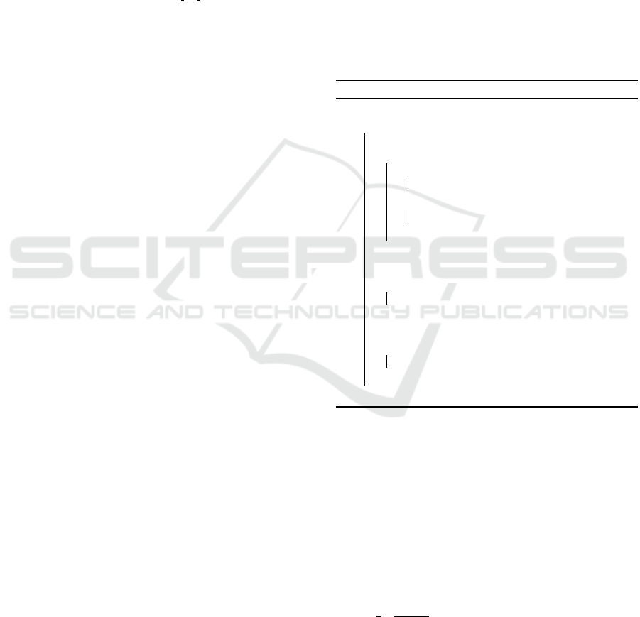
Figure 2: Camera locations of the Garden scene, the drjohn-
son scene and the truck scene. Here, the camera positions
are closely distributed around the table in the center of the
garden.
With this formulation, the scene extent is proportional
to the distance of the furthest camera location in rela-
tion to the average camera position. This makes the
optimization algorithm heavily dependent on the cap-
turing process of the scene. If, for example, the cam-
era is orbiting around a small object within a large
environment, the scene extent can be very small, al-
though the scene is very large. An example for this
is shown in Figure 2 with the Garden scene of Mip-
NeRF360. Here all of the cameras are close to the
center, leading to a very small scene extent.
Subsequently a proportionally large outdoor scene
like Garden obtains a smaller scene extent than a pro-
portionally small indoor scene like Drjohnson, where
cameras are distributed throughout the entire volume.
The scene extent so far only reflects the distance of
camera positions but not the actual scene volume.
During training, this bias will lead to some Gaussians
being split or pruned, even though they might be sized
appropriately for such a big scene.
To encounter this, we propose a corrected scene,
that is not dependent on the camera locations, but in-
stead dependent on the SfM point cloud that is used as
an initialization for 3DGS. Specifically, we formulate
the new scene extent as follows:
e
′
scene
=
1
N
SfM
N
SfM
∑
i=1


C − p
i


2
(11)
Here N
SfM
is the number of SfM points p, and C
is the averaged camera position from Equation 10.
Overall, this correction provides a scene extent of
VISAPP 2025 - 20th International Conference on Computer Vision Theory and Applications
614

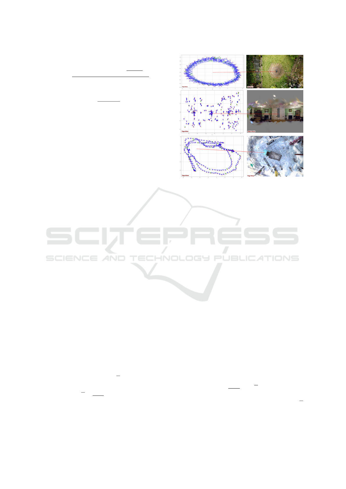
Figure 3: Our proposed gradient threshold schedule over
the densification interval compared against the number of
Gaussians created by our model. The number of densified
Gaussians clearly corresponds to our exponential schedule.
the same order of magnitude, better corresponding to
the naturally perceived extent for each scene.
4.2 Exponentially Ascending Gradient
Threshold
To control the number of Gaussians split or cloned
during densification, 3DGS compares the accumu-
lated positional gradient of each splat against a pre-
defined threshold. Gaussians with high gradients, in-
dicating frequent movement during optimization, are
selected for densification. Intuitively, this approach
assumes that if a Gaussian moves frequently, it is ef-
fectively filling multiple places at once. Splitting or
cloning these Gaussians distributes the work on two
separate Gaussians.
In 3DGS, this threshold is set to the fixed value of
0.0002. We argue that this setting is not ideal for fast
convergence. Specifically, during early optimization
steps, only few Gaussians exist in the scene, hindering
convergence without spawning new Gaussians. Vice
versa, at the end of the training, the scene is already
constructed of many Gaussians, where additional den-
sification can lead to overfitting. To encounter both
problems, we propose an ascending gradient thresh-
old that starts at a low value of 0.0001, allowing many
Gaussians to densify during the beginning, and ends
at a high value of 0.0004, where only those Gaussians
with a very high positional gradient are cloned and
split. Figure 3 visualizes that schedule and its impli-
cations for the densification process. The exponential
scheduling for the threshold T
i
in iteration i can be
described as follows:
T
i
= exp

ln(T
s
) · (1 −
i
i
max
) + ln(T
f
) ·
i
i
max

(12)
Here i
max
denotes the number of iterations, T
s
is
the initial, and T
f
the final value for the gradient
threshold. As shown in Figure 4, with this configu-
ration, the number of Gaussians rises much quicker,
Figure 4: Number of Gaussians during the training. With
our proposed exponentially ascending gradient threshold,
we produce many Gaussians at the beginning of the training
and few at the end. Here, we trained with the Drjohnson
scene.
compared to 3DGS and PixelGS, during early train-
ing steps, while it declines towards the end. After
15000, the densification stops and our method pro-
duces a similar number of Gaussians as 3DGS.
4.3 Significance-Aware Pruning
In 3D Gaussian Splatting, the primary objective of
pruning lies in reducing the overhead caused by stor-
ing and processing unnecessary Gaussians that do not
effectively contribute to scene reconstruction. How-
ever, finding those specific Gaussians remains a chal-
lenge. Unless the opacity or the scale of a Gaussian
is set to zero, it is not trivial whether the Gaussian
can be removed without harming the rendering qual-
ity. Figure 5 indicates that the baseline pruning al-
gorithm performs pruning decisions conflicting with
scene reconstruction.
An effective pruning algorithm therefore should
minimize the chance of pruning Gaussians that are
essential for scene reconstruction. We propose an
improved pruning strategy that effectively balances
the trade-off between reconstruction quality and scene
compactness by more accurately considering a Gaus-
sians contribution to the scene.
The pruning algorithm in 3DGS consists of size
and opacity pruning. We, however, observe that size
pruning has an adverse effect on both, scene recon-
struction and scene compactness. By removing a
large Gaussian from the scene, multiple small Gaus-
sians end up replacing it, thus increasing the overall
number of Gaussians in the scene. Moreover, a large
Gaussian with high opacity essentially contributes to
scene reconstruction. Therefore, simply removing
them most likely damages existing scene structures.
On the other, Opacity pruning only takes a Gaus-
sian’s opacity o
k
into account. However, this ap-
Improving Adaptive Density Control for 3D Gaussian Splatting
615

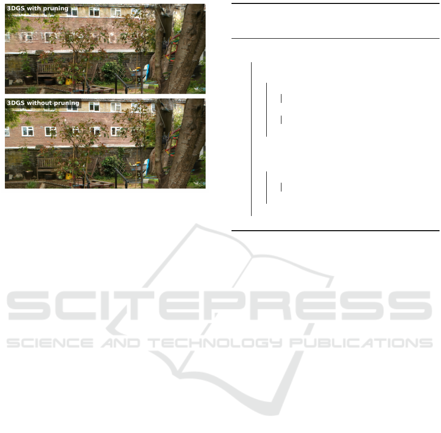
Figure 5: Selected novel view from the Garden scene
trained with the baseline (3DGS) in two configurations, one
with and the other without pruning.
proach does not fully reflect a Gaussian’s contribu-
tion to the scene. If a Gaussian g
k
has a large extent,
it has a more significant impact on alpha blending and
color
p
, especially if it contributes with high transmit-
tance t
k
. Therefore, the indicator that best reflects a
Gaussian’s contribution is the alpha blending coeffi-
cient w
k
.
To account for this discrepancy our proposed
pruning algorithm integrates both, a Gaussians opac-
ity o
k
and a Gaussians alpha blending coefficient w
k
into the pruning decision. Our pruning method first
selects all N
prune
Gaussians with opacities below o
min
.
From this selection, it then prunes only those Gaus-
sians with accumulated w
k
values within the bottom
N
prune
.
σ
k
=
N
pixel
∑
p=1
w
p
k
(13)
Σ = {σ
1
, ·· · , σ
n
} (14)
This accumulation σ
k
is computed over all N
pixel
pixels of all views between two densification steps.
This approach spares Gaussians with low opacity but
high significance to the scene reconstruction.
Over all, by considering both opacity o
k
and al-
pha blending coefficients w
k
in the pruning decision,
our approach evaluates a Gaussians contribution to
the scene more precisely. This precise evaluation en-
ables performing reliable pruning decisions through-
out scene training. Hence our method more effec-
tively optimizes the tradeoff between reconstruction
quality and scene compactness.
Algorithm 2: Our revised Densify and Prune Algorithm
with the corrected scene extent e
′
scene
, the exponential as-
cending gradient threshold T
i
and the significance pruning.
Data: Scene of Gaussians G
for g
k
∈ G do
//Densification
if τ
′
k
≥ T
i
then
if max(s
k
) > P
dense
· e
′
scene
then
splitGaussian(g
k
);
else
cloneGaussian(g
k
);
end
end
//Significance Pruning
if o
k
< o
min
then
if σ
k
∈ bottom(N
prune
, Σ) then
pruneGaussian(g
k
);
end
end
end
5 EXPERIMENTS
Combining these efforts yields Algorithm 2, which
we implemented into our model. For comput-
ing pixel-aware and depth-scaled 2D gradients we
rely on implementations provided by (Zhang et al.,
2024), without modifying any predetermined param-
eters. The Git repository containing all adapta-
tions is available at https://github.com/fraunhoferhhi/
Improving-ADC-3DGS.
For qualitative and quantitative evaluation, we
used the 3DGS evaluation pipeline provided by
(Kerbl et al., 2023). Our method was tested on all
real-world scenes shared by the authors, along with
the precomputed Structure-from-Motion (SfM) point
clouds used for initialization. These scenes include
Drjohnson and Playroom from Deep Blending (Hed-
man et al., 2018), nine scenes from MipNeRF 360
(Barron et al., 2021), and the Train and Truck scenes
from Tanks and Temples (Knapitsch et al., 2017).
We retained every eighth image from the pro-
vided input images as test images and computed Peak
Signal-to-Noise Ratio (PSNR), Structural Similarity
Index (SSIM), and Learned Perceptual Image Patch
Similarity (LPIPS) (Zhang et al., 2018) for these test
images.
Except for the adaptations discussed in Section 4,
we left all hyperparameters at the default values used
in 3DGS. All scenes were trained with identical con-
figurations to ensure consistency across evaluations.
VISAPP 2025 - 20th International Conference on Computer Vision Theory and Applications
616

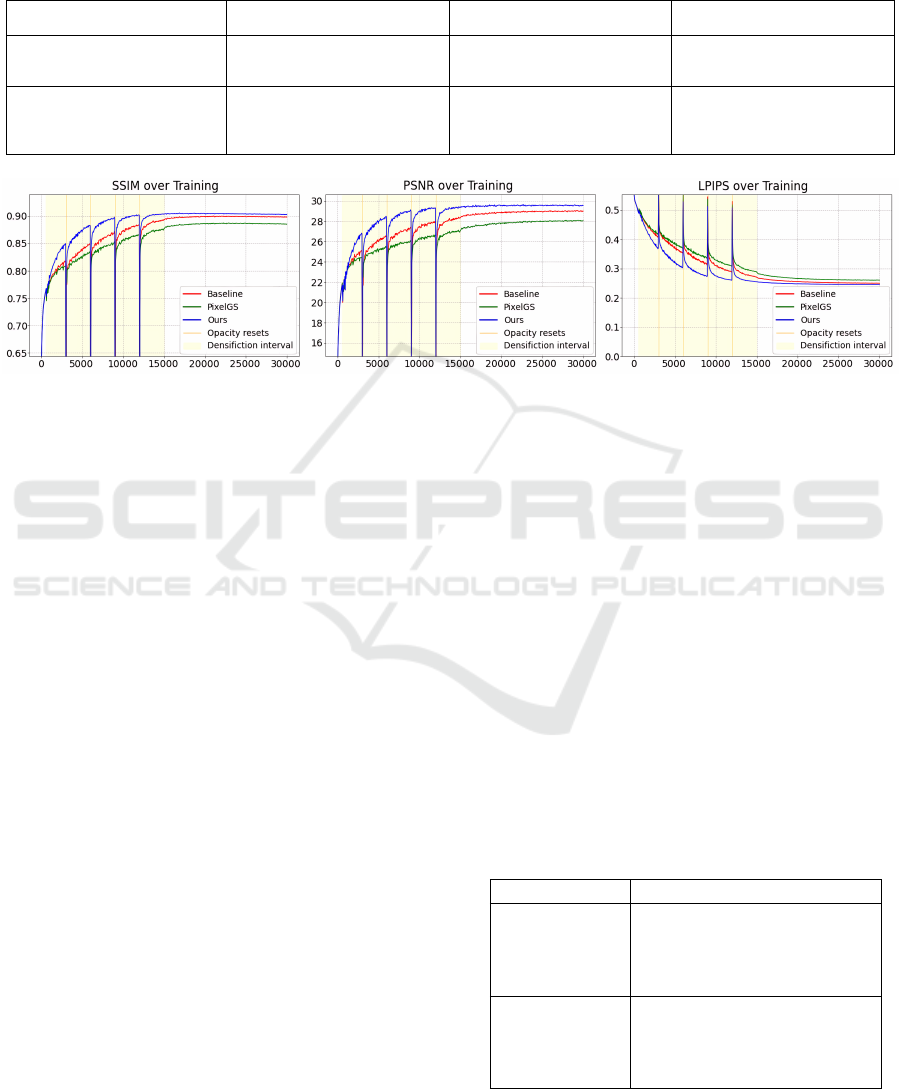
Table 1: Metrics and number of Gaussians averaged over all scenes from, MipNeRF 360 (Barron et al., 2021), Tanks and
Temples (Knapitsch et al., 2017) and Deep Blending (Hedman et al., 2018) datasets respectively. We retrieved metrics for
Plenoxels (Fridovich-Keil and Yu et al., 2022), INGP (M
¨
uller et al., 2022), and MipNeRF (Barron et al., 2021) from (Kerbl
et al., 2023). The LPIPS score for Revising Densification (Bul
`
o et al., 2024) is missing, since they use a different LPIPS
calculation that is not publicly available.
Dataset Mip-NeRF 360 Tanks and Temples Deep Blending
Method / Metric PSNR↑ SSIM↑ LPIPS↓ #Gaussians↓ PSNR↑ SSIM↑ LPIPS↓ #Gaussians↓ PSNR↑ SSIM↑ LPIPS↓ #Gaussians↓
Plenoxels 23.08 0.626 0.463 21.08 0.719 0.379 23.06 0.895 0.51
INGP-Big 25.59 0.699 0.331 21.92 0.745 0.305 24.96 0.817 0.390
MipNeRF 27.69 0.792 0.237 22.22 0.759 0.257 29.40 0.901 0.245
3DGS 27.39 0.813 0.218 3.3M 23.74 0.846 0.178 1.8M 29.50 0.899 0.247 2.8M
PixelGS (Zhang et al., 2024) 27.53 0.822 0.191 5.5M 23.83 0.854 0.151 4.5M 28.95 0.892 0.250 4.6M
Revising Dens. (Bul
`
o et al., 2024) 27.61 0.822 3.3M 23.93 0.853 1.8M 29.50 0.904 2.8M
Ours 27.71 0.824 0.193 3.3M 24.18 0.860 0.149 2.4M 29.63 0.902 0.240 2.3M
Figure 6: Comparison of the metrics over all test images achieved by the baseline (3DGS) (Kerbl et al., 2023), PixelGS (Zhang
et al., 2024), and Ours for the Drjohnson scene. PixelGS struggles with misplaced Gaussians, harming reconstruction quality.
5.1 Quantitative Evaluation
As we directly benefit from the work of (Zhang et al.,
2024) and (Bul
`
o et al., 2024), incorporating imple-
mentations from their proposed methods, we evalu-
ate our method against theirs. Table 1 presents the
evaluation metrics and the number of Gaussians used
for scene reconstruction across 3DGS, PixelGS, Re-
vising Densification in Gaussian Splatting and our
method. To provide further context for our results,
we have also included metrics for previous radiance
field methods such as Plenoxels (Fridovich-Keil and
Yu et al., 2022), INGP (M
¨
uller et al., 2022), and Mip-
NeRF (Barron et al., 2021).
Our method consistently outperforms the baseline
across all three datasets and evaluation metrics, us-
ing a comparable number of Gaussian primitives for
scene representation. Moreover, we surpass PixelGS
and Revising Densification in Gaussian Splatting in
almost all metrics across all datasets. Notably, our
method achieves these results using only about half
the number of Gaussians required by PixelGS.
In addition to the metrics reported in Table 1, we
also highlight the rendering quality during training in
Figure 6. Here, our method (blue) clearly outperforms
3DGS and PixelGS especially at the beginning of the
training. After only 10k training iterations, the PSNR
is already higher than the PSNR of the other methods
after 30k iterations. After half of the training steps at
15k iterations, our method reaches a state where the
quality does not improve much further. This suggests
that with our method much shorter training times are
possible without losing a lot of quality. To support
this, we also report the rendering quality metrics af-
ter 15k iterations in Table 2. Here, we observe con-
siderably higher rendering quality when using our
method. Furthermore, we also compare the qual-
ity between the models trained with 15k iterations
to models trained with 30k iterations. Notably, our
method already exceeds the final quality of 3DGS and
PixelGS with only 15k training steps.
Training the scene with half of the iterations leads
to a training time reduction in more than half of the
time. This is because earlier training iterations take up
less time since fewer Gaussians have to be rendered.
Table 2: Rendering quality metrics when using 15k training
iterations vs 30k iterations averaged over three scenes (one
from each dataset).
PSNR↑ SSIM↑ LPIPS↓
15K Iterations
3DGS 26.63 0.870 0.191
PixelGS 26.33 0.869 0.183
Ours 27.27 0.882 0.167
30K Iterations
3DGS 27.23 0.878 0.174
PixelGS 27.00 0.877 0.164
Ours 27.65 0.886 0.156
Improving Adaptive Density Control for 3D Gaussian Splatting
617

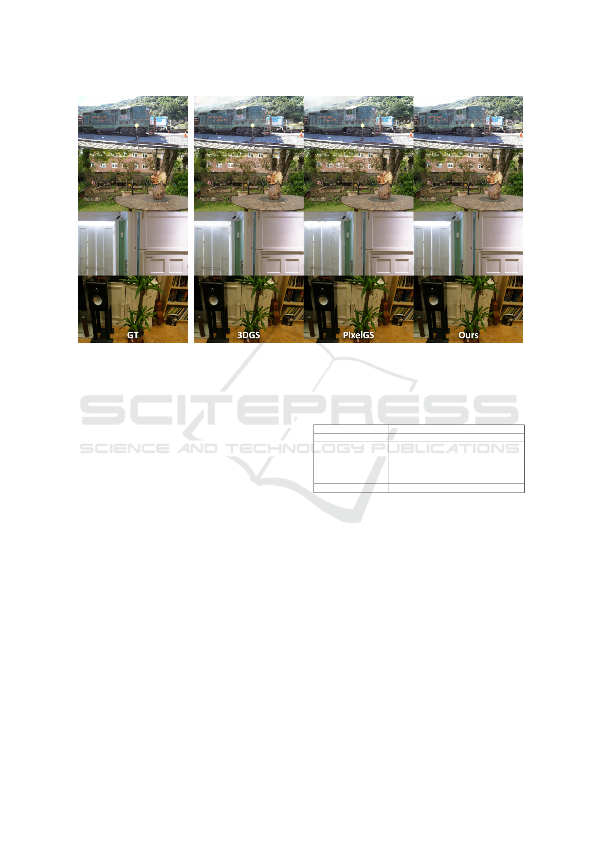
Figure 7: Visual comparison between 3DGS, PixelGS and our method along with the corresponding ground truth. Our method
shows less artifacts especially in background regions (first two rows) and less over-fitting noise (last two rows).
5.2 Qualitative Evaluation
To underline the quantitative results from Table 1,
Figure 7 presents a selection of test views rendered
using 3DGS, PixelGS and our method. As shown, our
method consistently outperforms the other methods in
terms of reconstruction quality. Our model excels at
capturing high-complexity regions in both the fore-
ground and background, where both 3DGS and Pix-
elGS tend to populate these areas with large, blurry
Gaussians. An example of improved background re-
gions can be seen in the second row of Figure 7. Here,
especially the windows of the building in the back-
ground look much less distorted using our method.
This is a similar result as shown in Figure 5, where
the model was trained without pruning. A better re-
construction in the foreground regions can be seen in
the last row. Focusing on the white door of the cup-
board we observe blurry regions when using 3DGS
and overfitted regions when using PixelGS. A simi-
lar observation can be made in the third row, looking
at the door on the left. Furthermore, we often observe
floating artifacts above the train in the first row, which
our method resolves. Further examples can be viewed
in the appendix.
5.3 Ablation Study
In total, our final method consists of five changed
components compared to the default implementation
Table 3: Results for the ablation study, where we deactivate
each of our three proposed components, as well as the pixel
gradient from PixelGS (Zhang et al., 2024) and the opacity
correnction from revising densification (Bul
`
o et al., 2024).
Method / Metric PSNR↑ SSIM↑ LPIPS↓ #Gaussians↓
Ours 27.46 0.841 0.194 3,021k
w/o extent correction 27.34 0.841 0.194 3,204k
w/o pruning strategy 27.37 0.841 0.194 3,097k
w/o exp grad thresh 27.45 0.842 0.195 3,143k
w/o opacity correction 27.30 0.839 0.191 4,755k
w/o pixel gradient 27.38 0.834 0.213 1,989k
3DGS 27.16 0.832 0.216 2,994k
of 3DGS (Kerbl et al., 2023). Those include our three
proposed methods, the pixel gradient from (Zhang
et al., 2024) and the adapted opacity from (Bul
`
o et al.,
2024). To evaluate the effectiveness of our final con-
figuration, we perform an ablation study in which we
deactivate each of the components in an isolated ex-
periment. The quantitative results for those experi-
ments can be viewed in Table 3. Here, we average all
results from 13 scenes across all datasets. Generally,
we observe that turning off any component directly
leads to worse PSNR performance. The highest de-
crease across our methods is found with the correc-
tion of the scene extent and the significance aware
pruning strategy. The exponential gradient thresh-
old, on the other hand, does not show a big difference
in PSNR. Nevertheless, deactivating the exponential
gradient threshold leads to more Gaussian splats be-
ing generated.
VISAPP 2025 - 20th International Conference on Computer Vision Theory and Applications
618

6 CONCLUSION
Gaussian Splatting has demonstrated its ability
to surpass state-of-the-art reconstruction methods
in quality; however, challenges such as under-
reconstruction, artifacts, and the omission of impor-
tant details, particularly in background regions high-
light areas for improvement. These limitations often
arise from imprecise densification. To address these
limitations, we build on recent advances in Adaptive
Density Control for 3DGS and propose several novel
improvements: a correction mechanism for scene ex-
tent, an exponentially ascending gradient threshold,
and significance-aware pruning.
Our comprehensive evaluation demonstrates that
combining these techniques effectively addresses
these challenges, resulting in improved reconstruc-
tion quality while maintaining a manageable number
of Gaussian primitives. Although some of the mod-
ifications only bring minor improvements, all of the
components are straightforward to implement into ex-
isting 3DGS frameworks, providing a practical and
efficient enhancement to previous methods.
ACKNOWLEDGEMENTS
This work has partly been funded by the Ger-
man Research Foundation (project 3DIL, grant
no. 502864329), the German Federal Ministry of
Education and Research (project VoluProf, grant
no. 16SV8705), and the European Commission (Hori-
zon Europe project Luminous, grant no. 101135724).
REFERENCES
Bagdasarian, M. T., Knoll, P., Li, Y.-H., Barthel, F., Hils-
mann, A., Eisert, P., and Morgenstern, W. (2024).
3dgs.zip: A survey on 3d gaussian splatting compres-
sion methods.
Barron, J. T., Mildenhall, B., Tancik, M., Hedman, P.,
Martin-Brualla, R., and Srinivasan, P. P. (2021). Mip-
nerf: A multiscale representation for anti-aliasing
neural radiance fields. ICCV.
Barthel, F., Beckmann, A., Morgenstern, W., Hilsmann, A.,
and Eisert, P. (2024). Gaussian splatting decoder for
3d-aware generative adversarial networks. In Pro-
ceedings of the IEEE/CVF Conference on Computer
Vision and Pattern Recognition (CVPR) Workshops,
pages 7963–7972.
Botsch, M., Sorkine-Hornung, A., Zwicker, M., and
Kobbelt, L. (2005). High-quality surface splatting on
today’s gpus. pages 17– 141.
Bul
`
o, S. R., Porzi, L., and Kontschieder, P. (2024). Revising
densification in gaussian splatting.
Fan, Z., Wang, K., Wen, K., Zhu, Z., Xu, D., and Wang, Z.
(2023). Lightgaussian: Unbounded 3d gaussian com-
pression with 15x reduction and 200+ fps.
Fang, G. and Wang, B. (2024). Mini-splatting: Represent-
ing scenes with a constrained number of gaussians. In
Leonardis, A., Ricci, E., Roth, S., Russakovsky, O.,
Sattler, T., and Varol, G., editors, Computer Vision –
ECCV 2024, pages 165–181, Cham. Springer Nature
Switzerland.
Fridovich-Keil and Yu, Tancik, M., Chen, Q., Recht, B.,
and Kanazawa, A. (2022). Plenoxels: Radiance fields
without neural networks. In CVPR.
Hedman, P., Philip, J., Price, T., Frahm, J.-M., Drettakis,
G., and Brostow, G. (2018). Deep blending for
free-viewpoint image-based rendering. ACM Trans.
Graph., 37(6).
Kerbl, B., Kopanas, G., Leimk
¨
uhler, T., and Drettakis,
G. (2023). 3d gaussian splatting for real-time radi-
ance field rendering. ACM Transactions on Graphics,
42(4).
Kim, S., Lee, K., and Lee, Y. (2024). Color-cued efficient
densification method for 3d gaussian splatting. In Pro-
ceedings of the IEEE/CVF CVPR Workshops, pages
775–783.
Kingma, D. P. and Ba, J. (2017). Adam: A method for
stochastic optimization.
Knapitsch, A., Park, J., Zhou, Q.-Y., and Koltun, V. (2017).
Tanks and temples: benchmarking large-scale scene
reconstruction. ACM Trans. Graph., 36(4).
Liu, K., Zhan, F., Xu, M., Theobalt, C., Shao, L., and Lu, S.
(2024). Stylegaussian: Instant 3d style transfer with
gaussian splatting. arXiv preprint arXiv:2403.07807.
Luiten, J., Kopanas, G., Leibe, B., and Ramanan, D. (2024).
Dynamic 3d gaussians: Tracking by persistent dy-
namic view synthesis. In 3DV.
Mildenhall, B., Srinivasan, P. P., Tancik, M., Barron, J. T.,
Ramamoorthi, R., and Ng, R. (2020). Nerf: Repre-
senting scenes as neural radiance fields for view syn-
thesis. In ECCV.
M
¨
uller, T., Evans, A., Schied, C., and Keller, A. (2022).
Instant neural graphics primitives with a multiresolu-
tion hash encoding. ACM Trans. Graph., 41(4):102:1–
102:15.
Pfister, H., Zwicker, M., van Baar, J., and Gross, M.
(2000). Surfels: surface elements as rendering prim-
itives. In Proceedings of the 27th Annual Conference
on Computer Graphics and Interactive Techniques,
SIGGRAPH ’00, page 335–342, USA.
Ren, L., Pfister, H., and Zwicker, M. (2002). Object space
ewa surface splatting: A hardware accelerated ap-
proach to high quality point rendering. Computer
Graphics Forum, 21.
Zhang, R., Isola, P., Efros, A. A., Shechtman, E., and Wang,
O. (2018). The unreasonable effectiveness of deep
features as a perceptual metric.
Zhang, Z., Hu, W., Lao, Y., He, T., and Zhao, H. (2024).
Pixel-gs: Density control with pixel-aware gradient
for 3d gaussian splatting.
Zwicker, M., Pfister, H., Baar, J., and Gross, M. (2001).
Ewa volume splatting. IEEE Visualization.
Improving Adaptive Density Control for 3D Gaussian Splatting
619

APPENDIX
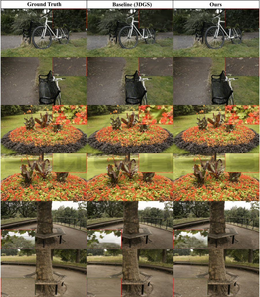
Figure 8: Rendered novel views for the Bicycle, Flowers, and Treehill scenes from the MipNeRF-360 dataset (Barron et al.,
2021) demonstrate that our model enables detailed reconstruction of intricate structures in both foreground and background
regions. In comparison, our approach significantly surpasses the baseline in terms of reconstruction quality.
VISAPP 2025 - 20th International Conference on Computer Vision Theory and Applications
620

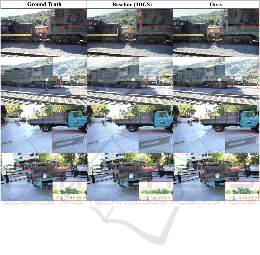
Figure 9: Rendered novel views for the Train and Truck scenes from the Tanks and Temples dataset (Knapitsch et al., 2017)
clearly demonstrate that our model improves reconstruction, particularly in background regions and near scene edges, while
reducing the number of artifacts. As a result, our approach significantly outperforms the baseline in terms of reconstruction
quality.
Improving Adaptive Density Control for 3D Gaussian Splatting
621