Online Importance Sampling for Stochastic Gradient Optimization
Corentin Sala
¨
un
1 a
, Xingchang Huang
1 b
, Iliyan Georgiev
2 c
, Niloy Mitra
2,3 d
and
Gurprit Singh
1 e
1
Max Planck Institute for Informatics, Saarland University, Saarbr
¨
ucken, Germany
2
Adobe Research, London, U.K.
3
Department of Computer Science, University College London, London, U.K.
Keywords:
Optimization, Machine Learning, Gradient Estimation.
Abstract:
Machine learning optimization often depends on stochastic gradient descent, where the precision of gradient
estimation is vital for model performance. Gradients are calculated from mini-batches formed by uniformly
selecting data samples from the training dataset. However, not all data samples contribute equally to gradient
estimation. To address this, various importance sampling strategies have been developed to prioritize more
significant samples. Despite these advancements, all current importance sampling methods encounter chal-
lenges related to computational efficiency and seamless integration into practical machine learning pipelines.
In this work, we propose a practical algorithm that efficiently computes data importance on-the-fly during
training, eliminating the need for dataset preprocessing. We also introduce a novel metric based on the deriva-
tive of the loss w.r.t. the network output, designed for mini-batch importance sampling. Our metric prioritizes
influential data points, thereby enhancing gradient estimation accuracy. We demonstrate the effectiveness of
our approach across various applications. We first perform classification and regression tasks to demonstrate
improvements in accuracy. Then, we show how our approach can also be used for online data pruning by
identifying and discarding data samples that contribute minimally towards the training loss. This significantly
reduce training time with negligible loss in the accuracy of the model.
1 INTRODUCTION
Stochastic gradient descent (SGD) combined with
back-propagation has driven significant advances in
optimization tasks. Its strength lies in its ability to
optimize complex models by iteratively updating their
parameters based on the gradient of the loss function.
However, despite its widespread use, SGD has no-
table limitations. Convergence rates are influenced by
several factors, with gradient noise being a key chal-
lenge that affects both robustness and convergence
speed. Reducing this noise has been a focus of recent
research (Alain et al., 2015; Faghri et al., 2020; John-
son and Zhang, 2013; Gower et al., 2020; Needell
et al., 2014).
Various strategies have been proposed to mitigate
a
https://orcid.org/0000-0002-5112-7488
b
https://orcid.org/0000-0002-2769-8408
c
https://orcid.org/0000-0002-9655-2138
d
https://orcid.org/0000-0002-2597-0914
e
https://orcid.org/0000-0003-0970-5835
gradient noise, including data diversification (Zhang
et al., 2017; Zhang et al., 2019), adaptive batch sizes,
weighted sampling (Santiago et al., 2021), and impor-
tance sampling (Katharopoulos and Fleuret, 2018).
These approaches aim to enhance gradient estima-
tion and accelerate convergence in noisy optimization
landscapes.
This work focuses on both importance sam-
pling and data pruning as complementary tech-
niques to improve training efficiency. Importance
sampling involves constructing mini-batches through
non-uniform data-point selection, i.e., picking certain
data points with higher probability based on their ex-
pected contribution to the model’s learning process.
In parallel, data pruning seeks to identify and elimi-
nate data points that contribute minimally to training,
reducing computational load. This is especially ben-
eficial in large-scale learning tasks, where reducing
data complexity can significantly improve both time
and resource efficiency. By jointly leveraging these
two techniques, we aim to both improve the accuracy
of gradient estimates and streamline the training pro-
130
Salaün, C., Huang, X., Georgiev, I., Mitra, N. and Singh, G.
Online Importance Sampling for Stochastic Gradient Optimization.
DOI: 10.5220/0013311100003905
Paper published under CC license (CC BY-NC-ND 4.0)
In Proceedings of the 14th International Conference on Pattern Recognition Applications and Methods (ICPRAM 2025), pages 130-140
ISBN: 978-989-758-730-6; ISSN: 2184-4313
Proceedings Copyright © 2025 by SCITEPRESS – Science and Technology Publications, Lda.

cess by focusing computation resources on valuable
data.
In this paper, we introduce a novel metric that
quantifies the contribution of each data sample to the
model’s learning process, to guide both importance
sampling and data pruning decisions. Our approach
leverages information from the network’s output to
strategically allocate computational resources to the
most impactful data points. This results in substan-
tial improvements in convergence across a variety of
tasks, while sustaining minimal computational over-
head compared to state-of-the-art methods that share
similar goals (Katharopoulos and Fleuret, 2018; San-
tiago et al., 2021).
In summary, our contributions can be distilled into
the following key points:
• We propose an adaptive metric for importance
sampling improving gradient accuracy.
• We introduce an efficient online sampling algo-
rithm that incorporates our metric.
• We demonstrate the effectiveness of our approach
through evaluations on classification and regres-
sion problems.
• We further demonstrate the ability of our al-
gorithm to perform online data pruning. Our
approach allows using any importance function
for data pruning and does not require any pre-
processing of the data.
2 RELATED WORK
Gradient estimation is a cornerstone in machine learn-
ing, underpinning the optimization of models. In
practical scenarios, computing the exact gradient is
infeasible due to the sheer volume of data, leading to
the reliance on mini-batch approximations. Improv-
ing these approximations to obtain faster and more
accurate estimates remains a challenge. The ultimate
goal is to accelerate gradient descent by using more
accurate gradient estimates.
Importance Sampling. Importance sampling
serves as a mechanism for error reduction in mini-
batch gradient estimation. Each data point is assigned
a probability to be selected in each mini-batch, mak-
ing some data more likely to be chosen than others.
(Bordes et al., 2005) developed an online algorithm
(LASVM) which uses importance sampling to train
kernelized support vector machines. Several studies
have shown that importance sampling proportional
to the gradient norm is the optimal sampling strategy
(Zhao and Zhang, 2015; Needell et al., 2014; Wang
et al., 2017; Alain et al., 2015). (Hanchi et al., 2022)
recently proposed deriving an importance sampling
metric from the gradient norm of each data point,
demonstrating favorable convergence properties
and provable improvements under certain convexity
conditions.
Estimating the gradient for each data point can
be computationally intensive. Thus, the search for
more efficient sampling strategies has led to the ex-
ploration of efficient approximations of the gradient
norm. Methods proposed by (Loshchilov and Hut-
ter, 2015) rank data based on their loss and derive
an importance sampling strategy assigning higher im-
portance to data with higher loss. (Katharopoulos and
Fleuret, 2017) proposed importance sampling the loss
function. Additionally, (Dong et al., 2021) proposed
a resampling-based algorithm to reduce the number
of backpropagation computations, selecting a subset
of data based on the loss. Similarly, (Zhang et al.,
2023) proposed resampling based on multiple heuris-
tics to reduce the number of backward propagations
and focus on more influential data. (Katharopoulos
and Fleuret, 2018) introduced an upper bound to the
gradient norm that can be used as an importance func-
tion, suggesting re-sampling data based on impor-
tance computed at the last layer. These resampling
methods reduce unnecessary backward propagations
but still require forward computation for each data
point.
Data Weighting. An alternative to importance sam-
pling is to adjust the contribution of uniformly se-
lected data points by a weighting factor. To compute
weights within a mini-batch, (Santiago et al., 2021)
proposed a method maximizing the mini-batch’s ef-
fective gradient. This allocation of weights aims to
align data contributions with the optimization objec-
tive, expediting convergence at the cost of potential
bias.
Data Pruning. Data pruning reduces the computa-
tional load of training by removing minimally useful
data. Early work by (Har-Peled and Kushal, 2005)
proposed using a smaller, representative dataset for k-
means clustering. This concept has expanded to other
machine learning tasks, where not all data points con-
tribute equally to learning. (Toneva et al., 2019) found
that some data points, once correctly classified, re-
main so, suggesting they can be pruned without af-
fecting performance.
(Coleman et al., 2020) introduced a proxy network
to guide pruning by selecting relevant data points
based on predictions. (Paul et al., 2021) further re-
fined this strategy by using early training informa-
Online Importance Sampling for Stochastic Gradient Optimization
131

tion to identify important data points, allowing train-
ing on smaller data subsets with small performance
loss. These methods show that focusing on the most
informative samples can enhance training efficiency.
(Yang et al., 2023) proposed to select a subset of the
dataset and propose a discrete optimization method
using influence functions to determine which data
points to retain and which to prune from the train-
ing dataset. Unfortunately, their overall preprocess-
ing can take hours and does not scale well to large
datasets. In contrast, our importance sampling algo-
rithm can be used for online data pruning without any
preprocessing. (Qin et al., 2023) proposed an online
data pruning method based on loss of data samples
with an additional re-scaling of the sample gradient.
3 BACKGROUND
In machine learning, the goal is to find the optimal set
of parameters θ for a model function m(x,θ), with x
a data sample (and y its supervision label), that min-
imize a loss function L over a dataset Ω. The opti-
mization is typically expressed as
θ
∗
= argmin
θ
L
θ
, where (1)
L
θ
=
1
|Ω|
Z
Ω
L (m(x,θ), y)d(x,y) = E

L (m(x,θ), y)
p(x,y)

.
The total loss L
θ
can be interpreted in two ways. The
analytical interpretation views it as the integral of the
loss L over a data space Ω, normalized by the space’s
volume. In machine learning, the data space typically
represents the (discrete) training dataset and the nor-
malization is its size. The second, statistical inter-
pretation defines L
θ
as the expected value of the loss
L for a randomly selected data point, divided by the
probability of selecting it. The two approaches are
equivalent.
In practice, the minimization of the total loss L
θ
is tackled via iterative gradient descent. At each iter-
ation t, its gradient ∇L
θ
t
with respect to the current
model parameters θ
t
is computed, and those parame-
ters are updated as
θ
t+1
= θ
t
− λ∇L
θ
t
, (2)
where λ > 0 is the learning rate. The learning rate
does not need to remain constant throughout the itera-
tions and can be adjusted accordingly. The procedure
is repeated until a convergence criterion is met or for
a predefined number of iterations.
3.1 Monte Carlo Gradient Estimator
Gradient Estimator. The parameter update
in Eq. (2) involves evaluating the total-loss gradient
∇L
θ
t
. This requires processing the entire dataset Ω
at each of potentially many (thousands of) steps,
making the optimization computationally infeasible.
In practice one has to resort to mini-batch gradient
descent at each iteration which estimates the gradient
from a small set {x
i
}
B
i=1
⊂ Ω of randomly chosen
data points from the entire dataset in a Monte Carlo
fashion:
∇L
θ
≈
1
B
∑
B
i=1
∇L (m(x
i
,θ),y
i
)
p(x
i
,y
i
)
= ⟨∇L
θ
⟩, with x
i
∝ p(x
i
).
(3)
Here, ∇L (m(x
i
,θ),y
i
) is the gradient (w.r.t. θ) of the
loss function for sample x
i
selected following a prob-
ability density function (pdf) p (or probability mass
function in case of a discrete dataset). Any distribu-
tion p ensuring that p(x) = 0 ⇒ ∇L (m(x
i
,θ),y
i
) = 0
yields an unbiased gradient estimator, i.e., E[⟨∇L
θ
⟩] =
∇L
θ
. The sampling of the multiple data of a mini-
batch is done with replacement to ensure all data are
selected flowing the same probability density p(x).
Mini-batch gradient descent uses ⟨∇L
θ
⟩ in place of
the true gradient ∇L
θ
in Eq. (2) to update the model
parameters at every optimization iteration. The batch
size B is typically much smaller than the dataset, en-
abling practical optimization.
Theoretical Convergence Analysis. Mini-batch
gradient descent is affected by Monte Carlo noise due
to the stochastic gradient estimation in Eq. (3). This
noise arises from the varying contributions of differ-
ent samples x
i
to the estimate and can cause the pa-
rameter optimization trajectory to be erratic, slowing
down convergence. In certain conditions, it is pos-
sible to express the convergence rate of such meth-
ods. (Gower et al., 2019) demonstrated that for an L-
smooth and µ-convex function, the convergence rate
of mini-batch gradient descent with constant learning
rate is
E
h
∥
θ
t
− θ
∗
∥
2
i
≤ (1 − λµ)
t
∥
θ
0
− θ
∗
∥
2
+
2λσ
2
µ
, (4)
with σ
2
= E
h
∥
⟨∇L
θ
∗
⟩
∥
2
i
−
=0
z }| {
E[
∥
⟨∇L
θ
∗
⟩
∥
]
2
and it’s
value depends on the choice of norm. The expected
value of the gradient norm is zero for the optimal set
of parameters θ
∗
, as the solution of the gradient de-
scent is reached when the gradient converges to zero.
This equation underscores the significance of mini-
mizing variance in gradient estimation to enhance the
convergence rate of gradient descent methods. While
not universally applicable, it provides valuable in-
sights into expected behavior when reducing estima-
tion errors. Hence, refining gradient estimates is cru-
cial for optimizing various learning algorithms, facili-
ICPRAM 2025 - 14th International Conference on Pattern Recognition Applications and Methods
132

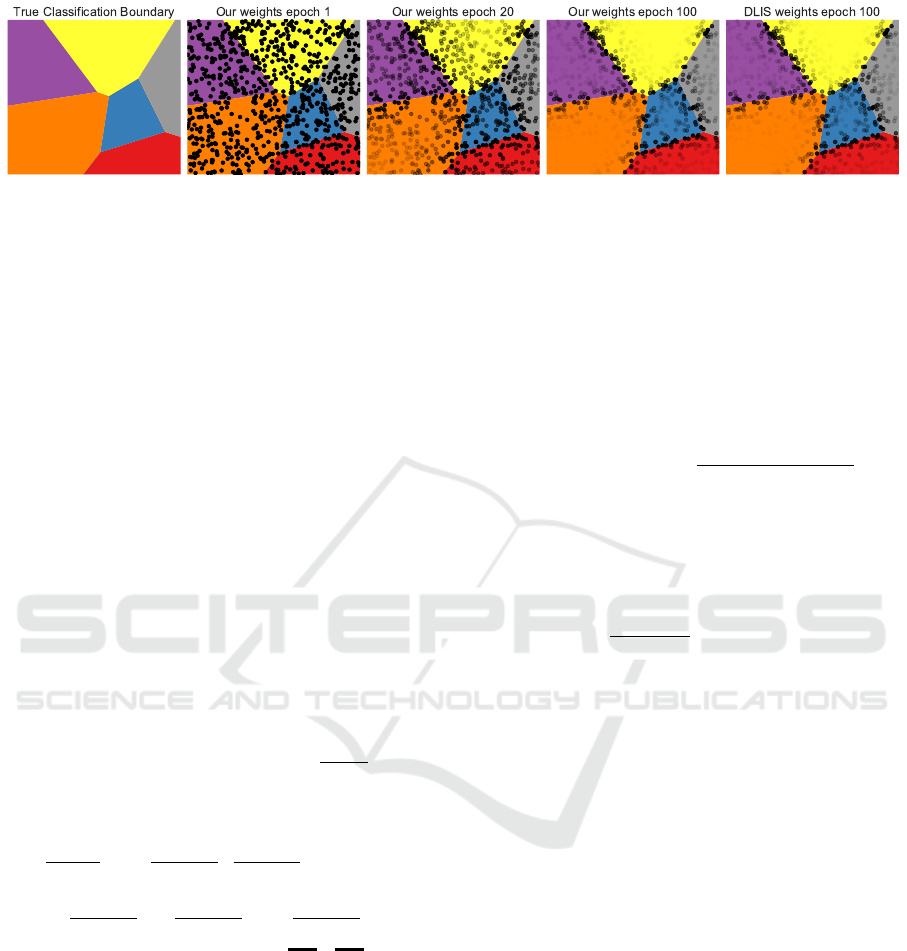
Figure 1: Visualization of the importance sampling at 3 different epoch and the underlying classification task. For each
presented epoch, 800 data-point are presented with a transparency proportional to their weight according to our method. At
epoch 800 our weights show high similarity to DLIS method while in practice some discrepancy differentiate the two method
but are not visible in this simple example.
tating more efficient convergence towards optimal so-
lutions. Our experimental evaluation comparing dif-
ferent methods in Section 4.2 further supports this no-
tion.
4 IMPORTANCE FUNCTION
4.1 Gradient Norm Bound
The gradient L
2
norm has been shown to be an opti-
mal choice of importance sampling (Zhao and Zhang,
2015; Needell et al., 2014; Wang et al., 2017; Alain
et al., 2015) as it minimizes the first term of the gra-
dient variance, thereby bounding the convergence of
Eq. (4). However, calculating it requires costly full
backpropagation for every data point, which is what
we want to avoid in the first place. Instead, we com-
pute an upper bound of the gradient L
2
-norm using the
output nodes of the network: q(x) =



∂L (x)
∂m(x,θ)



. This
upper bound of the gradient norm is derived from the
chain rule and the Cauchy–Schwarz inequality:




∂L (x
i
)
∂θ




=




∂L (x)
∂m(x,θ)
·
∂m(x,θ)
∂θ




(5)
≤




∂L (x)
∂m(x,θ)




·




∂m(x,θ)
∂θ




≤




∂L (x)
∂m(x,θ)




| {z }
q(x)
·C ,
where C is the Lipschitz constant of the parameters
gradient. That is, our importance function is a bound
of the gradient magnitude based on the output-layer
gradient norm. For specific shapes of the output layer,
it is possible to derive a closed form expression. Be-
low we show such derivation for classification net-
works based on the cross-entropy loss.
Cross-Entropy Loss Gradient. Cross entropy is
the standard loss function in classification tasks. It
quantifies the dissimilarity between predicted prob-
ability distributions and actual class labels. Specif-
ically, for a multi-class classification task, cross en-
tropy is defined as:
L (m(x
i
,θ)) = −
J
∑
j=1
y
j
log(s
j
)
where s
j
=
exp(m(x
i
,θ)
j
)
∑
J
k=1
exp(m(x
i
,θ)
k
)
(6)
where m(x
i
,θ) is an output layer, x
i
is the input data
and J means the number of classes. It is possible to
express the derivative of the loss L with respect to the
network output m(x
i
,θ)
j
in a close form.
∂L
∂m(x
i
,θ)
j
= s
j
− y
j
(7)
This equation can be directly computed from the
network output without any graph back-propagation.
This make the computation of our importance func-
tion extremely cheap for classification tasks. Proof of
the derivation can be found in the Supplemental doc-
ument.
Importance sampling in classification emphasizes
gradients along classification boundaries, where pa-
rameter modifications have the greatest impact. Fig-
ure 1 illustrates this concept, showing iterative refine-
ment of the sampling distribution to focus on bound-
ary decisions in comparison to data within classes.
The rightmost column illustrates the sampling dis-
tribution of the DLIS method of (Katharopoulos and
Fleuret, 2018) at epoch 100. Both methods iteratively
increase the importance of the sampling around the
boundary decision compare to data inside the classes.
Our approach differs from that of (Katharopou-
los and Fleuret, 2018) in that we compute the gra-
dient norm with respect to the network’s output log-
its. This approach often allows gradient computation
without requiring back-propagation or graph compu-
tations, streamlining optimization.
Online Importance Sampling for Stochastic Gradient Optimization
133

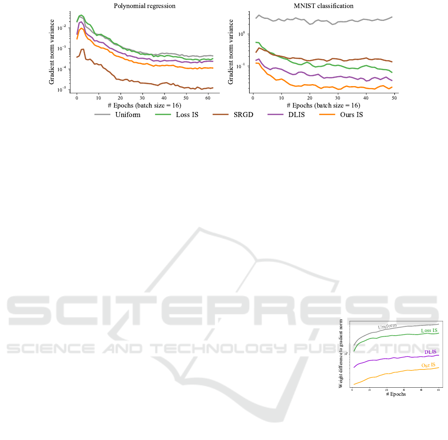
Figure 2: Evolution of gradient variance for variance importance sampling strategies on polynomial regression and MNIST
classification task. In both case the optimization is done on a 3 fully-connected layer network. Variance estimation is made
of each method on the same network at each epoch. The variance is computed using a mini-batch of size 16.
4.2 Convergence Analysis
Building on the theoretical bound defined in Eq. (4),
we proceed to examine the effects of various im-
portance sampling methods on the gradient variance.
Such variance influences the convergence of an opti-
mization procedure. This equation relies on the ideal
model parameters θ
∗
, but they cannot be practically
calculated. Rather, we measure the gradient variance
during training using a suboptimal parameter set.
Figure 2 displays the evolution of gradient vari-
ance using different strategies for polynomial regres-
sion and MNIST classification, both using a three-
layer fully connected network. Each method is eval-
uated on the same network, trained using uniform
sampling. This allows for a variances comparison
of the gradient norm. We analyze five techniques:
Uniform sampling, Loss-based importance sampling,
SRGD (Hanchi et al., 2022), DLIS (Katharopoulos
and Fleuret, 2018), and our method. SRGD is an
importance sampling technique using a conditioned
minimization of gradient variance using memory of
the gradient magnitude. This method has shown ro-
bust theoretical convergence properties in strongly
convex scenarios. This variance reduction is visi-
ble on the polynomial regression task where it result
in lower variance than other methods. However, for
more complex tasks such as MNIST classification,
SRGD underperforms all methods, suggesting scal-
ability limitations to non-convex and complex prob-
lems. In contrast, our method consistently yields
lower variance than Loss-based importance sampling
and DLIS (Katharopoulos and Fleuret, 2018). These
findings elucidate the results in Section 7.
In addition, we provide evaluation times for
each metric for both the polynomial regression
and MNIST classification tasks in Supplemental
document. Clearly, SRGD (Hanchi et al., 2022)
demands more computational resources, even for
small-scale networks comprising only three layers.
This increased demand stems from its dependence
on calculating the gradient norm for each individ-
ual data point. Both our metric, which employs
automatic differentiation, and DLIS (Katharopoulos
and Fleuret, 2018), incur comparable computational
costs due to their reliance on derivatives from the
final layers. Nonetheless, our approach proves to be
the most efficient when analytical evaluations are
feasible. Such differences in computational efficiency
are likely to significantly influence the outcomes of
comparisons made under equal-time conditions in
later sections.
(Zhao and Zhang,
2015) have shown
that importance
weights w.r.t. the
gradient norm
gives the optimal
sampling distri-
bution. On the right inline figure, we show the
difference between various weighting strategies
and the gradient norm w.r.t. all parameters. In this
experiment, all sampling weights are computed using
the same network on an MNIST optimization task.
Our proposed sampling strategies, based on the loss
gradient are the closest approximation to the gradient
norm.
5 ONLINE IMPORTANCE
SAMPLING ALGORITHM
We propose an algorithm to efficiently perform im-
portance sampling for mini-batch gradient descent,
outlined in Algorithm 1. Similarly to (Loshchilov and
Hutter, 2015) and (Schaul et al., 2015), it is designed
to use an importance function that relies on readily
available quantities for each data point, introducing
ICPRAM 2025 - 14th International Conference on Pattern Recognition Applications and Methods
134

only negligible memory and computational overhead
over classical uniform mini-batching.
Algorithm 1: Mini-batch importance sampling for SGD.
1: θ ← random parameter initialization
2: B ← mini-batch size, N = |Ω| ← Dataset size
3: q, θ ← Initialize(Ω,θ,B) ← see Supplemental
4: until convergence do ← Loop over epochs
5: for t ← 1 to N/B ← Loop over mini-batches
6: p ← q/sum(q) ← Normalize importance to pdf
7: x,y ← B data samples {x
i
,y
i
}
B
i=1
∝ p
8: L (x) ← L (m(x,θ),y)
9: ∇L (x) ← Backpropagate(L(x))
10: ⟨∇L
θ
⟩ ← (∇L (x) · (
1
/p(x))
T
)/B ← Eq. (3)
11: θ ← θ − η⟨∇L
θ
⟩ ← SGD step
12: q(x) ← α · q(x) + (1 − α) ·



∂L (x)
∂m(x,θ)



13:
↱
Accumulate importance
14:
15: q ← q + ε
16:
↱
to ensures no data samples are forgotten indefinitely
17: return θ
We maintain a set of persistent un-normalized im-
portance scalars q = q
i
|Ω|
i=1
, continually updated dur-
ing optimization. Initially, we process all data points
once in the first epoch to determine their initial im-
portance (line 3). Subsequently, at each mini-batch
optimization step t, we normalize the importance val-
ues to obtain the probability density function (PDF)
p (line 6), and use it to sample B data points with
replacement (line 7). We then evaluate the loss for
each selected data sample (line 8) and backpropa-
gate to compute the corresponding loss gradient (line
9). Finally, we update the network parameters us-
ing the estimated gradient (line 11). Additionally, we
compute the sample importance for each data sam-
ple from the mini-batch and update the persistent
importance q (line 12). Various importance heuris-
tics such as the gradient norm (Zhao and Zhang,
2015; Needell et al., 2014; Wang et al., 2017; Alain
et al., 2015), the loss (Loshchilov and Hutter, 2015;
Katharopoulos and Fleuret, 2017; Dong et al., 2021)
or more advanced importance (Katharopoulos and
Fleuret, 2018) can be implemented to replace our
sampling metric in this line. To enhance efficiency,
our algorithm reuses the forward pass computations
made during line 8 to compute importance, updating q
only for the current mini-batch samples. The weight-
ing parameter α ensures weight stability as discussed
in Eq. (8).
At the end of each epoch (line 15), we add a small
value to the un-normalized weights of all data to en-
sure that every data point will be eventually evaluated,
even if its importance is deemed low by the impor-
tance metric.
It is importance to note that the initialization
epoch is done without importance sampling to ini-
tialize each sample importance. This does not create
overhead as it is equivalent to a classical epoch run-
ning over all data samples. While similar schemes
have been proposed in the past, they often rely on
a multitude of hyperparameters, making their practi-
cal implementation challenging. This has led to the
development of alternative methods like re-sampling
(Katharopoulos and Fleuret, 2018; Dong et al., 2021;
Zhang et al., 2023). Our proposed sampling strategy
has only a few hyperparameters. Tracking importance
across batches and epochs minimizes the computa-
tional overhead, further enhancing the efficiency and
practicality of the approach.
6 ONLINE DATA PRUNING
Data pruning is a technique aimed at reducing the size
of the dataset to accelerate training. The accelera-
tion can be attributed to two main factors. The first,
and most practical, relates to the execution speed of
training neural networks. When working with large
datasets, especially those with a relatively large mem-
ory footprint, it is often infeasible to store all data
directly in GPU memory. This necessitates frequent
data loading from slower storage mediums, which
can become a bottleneck and significantly slow down
training. By reducing the dataset size, less data needs
to be loaded during each training iteration, leading to
faster execution, even if the theoretical properties of
the training process remain unchanged. The second
factor contributing to faster training is theoretical. If
the pruned data points have a low gradient norm, re-
moving them increases the expected gradient norm of
the remaining data points. This, in turn, leads to larger
effective steps in the optimization process, thus accel-
erating convergence.
Given these two benefits, we propose a data prun-
ing strategy guided by our novel importance metric,
which serves as an estimate of the gradient norm for
each data point. Unlike most previous works that rely
on precomputed metrics or early-stage proxies, our
metric is adaptive throughout training and does not
require any precomputation. This allows us to dynam-
ically prune the dataset based on current information
about the importance of each data point.
Our approach involves an online pruning process
that operates as follows: After a certain number of
epochs, we ensure that the importance metric has been
calculated for all data points in the training set. At
Online Importance Sampling for Stochastic Gradient Optimization
135

Table 1: We compare the impact of our importance sampling algorithm with or without data pruning on classification tasks. We
compare on three different datasets: Point cloud, CIFAR-100 and Tiny-ImageNet. Our approach consistently outperform on
majority of datasets (see Supplemental document for more comparisons). Bold numbers represents the best scores, underlined
ones represent the second best.
Point cloud CIFAR-100 Tiny-ImageNet
Equal step Equal time Equal step Equal time Equal step Equal time
Method Loss (↓) Accuracy (↑) Loss Accuracy Loss Accuracy Loss Accuracy Loss Accuracy Loss Accuracy
Uniform 0.00505 82.3 0.00505 82.2 0.012 72.6 0.012 73.8 0.02176 47.4 0.02176 47.4
Loss IS 0.00495 82.6 0.00496 82.5 0.023 40.2 0.026 32.8 0.02237 45.2 0.02238 45.2
DLIS 0.00595 81.9 0.00603 81.8 0.015 62.0 0.015 60.8 0.03433 26.3 0.03433 26.3
DLIS weights
0.00481 82.6 0.00485 82.5 0.021 43.6 0.029 26.3 0.03454 26.1 0.02778 35.0
w/ Our algorithm
LOW 0.00572 82.6 0.01173 74.9 0.011 74.6 0.011 74.2 0.02344 43.5 0.02344 43.5
Our IS 0.00480 82.9 0.00480 82.9 0.011 74.3 0.012 74.3 0.02127 48.1 0.02123 48.5
Our IS
0.00478 83.2 0.00478 83.1 0.011 74.3 0.011 74.3 0.02193 47.1 0.02193 47.1
+ Data pruning
Algorithm 2: Subroutine for data pruning.
1: function ONLINEDATAPRUNING(Ω,q,K,ε)
2: ε ←
1
K|Ω|
∑
x∈Ω
q(x) ← Compute pruning threshold
3: Ω
′
← Ω
{q(x)>ε|∀x∈Ω}
4: return Ω
′
↱
Filter dataset to keep high importance data
this point, we identify and remove a portion of the
data with importance metrics significantly lower than
the average. Specifically, each data point’s impor-
tance is compared to the average importance across
the dataset. If a data point’s importance falls below a
threshold relative to the average, it is pruned from the
training set. This ensures that only data points with
low expected gradient norms are removed, while im-
portant data remains. Algorithm 2 depicts the pruning
subroutine, which processes the dataset Ω, the impor-
tance score for each data point q, and a reduction fac-
tor K. A higher reduction factor results in retaining
more data points, thus fewer data are pruned.
This process is flexible and can adapt to the dis-
tribution of importance values in the dataset. If the
dataset has a wide distribution of importance, with
only a few data points contributing significantly to
the optimization, a large portion of the dataset can
be pruned. Conversely, if all data points exhibit rela-
tively high importance, few or no data points will be
removed. Furthermore, since our importance metric is
adaptive, this pruning process can be applied multiple
times throughout training. By continually updating
the importance metric and pruning low-importance
data points, we maintain an efficient training set that
accelerates the learning process without compromis-
ing model performance.
7 EXPERIMENTS
In this section, we delve into the experimental out-
comes of our proposed algorithm and sampling strat-
egy. Our evaluations encompass diverse classification
and regression tasks. We benchmarked our approach
against those of (Katharopoulos and Fleuret, 2018)
and (Santiago et al., 2021), considering various varia-
tions in comparison. Distinctions in our comparisons
lie in assessing performance at equal steps/epochs
and equal time intervals. The results presented here
demonstrate the loss and classification error, com-
puted on test data that remained unseen during the
training process.
7.1 Implementation Details
We implement our method and all baselines in a
single PyTorch framework. Experiments run on
a workstation with an NVIDIA Tesla A40 graph-
ics card. The baselines include uniform sam-
pling, DLIS (Katharopoulos and Fleuret, 2018) and
LOW (Santiago et al., 2021). Uniform means that
we sample every data point from a uniform distribu-
tion. DLIS importance samples the data mainly de-
pending on the norm of the gradient on the last out-
put layer. We use functorch (Horace He, 2021) to ac-
celerate this gradient computation. LOW is based on
adaptive weighting that maximizes the effective gra-
dient of the mini-batch using the solver from (Van-
denberghe, 2010).
We evaluated our method on a range of tasks,
including image classification with MNIST, CIFAR-
10/100 (Krizhevsky et al., 2009), Tiny-ImageNet (Le
and Yang, 2015), and Oxford Flower-102 (Nilsback
and Zisserman, 2008), as well as Point cloud classifi-
cation (Qi et al., 2017) and regression tasks (Sitzmann
et al., 2020). Full details on the datasets used, along
with optimization parameters such as learning rate,
optimizer scheduler and the data pruning ratio and
frequency are provided in Supplemental document.
In all results involving pruning, the number of steps
per epoch remains consistent with the non-pruned ex-
periments. This ensures a fair comparison at equal
steps, meaning that with pruning, certain data points
ICPRAM 2025 - 14th International Conference on Pattern Recognition Applications and Methods
136

Remaining data Training time(s)
Method Accuracy (At end of opt.) (Pruning time)
Uniform - - 96.4% 100% 554 (0)
Random pruning - - 96.3% 60% 131 (3)
Random pruning - - 96.2% 43% 121 (2)
Random pruning - - 96.1% 35% 114 (1)
(Yang et al., 2023) - - 96.4% 60% 132 (2388)
(Yang et al., 2023) - - 96.3% 43% 128 (4825)
(Yang et al., 2023) - - 96.2% 35% 121 (9351)
Ours (K=8) —- 97.9% 62% (33%) 215 (3)
Ours (K=4) —- 98.1% 45% (15%) 214 (2)
Ours (K=2) —- 98.1% 34% (6%) 208 (2)
Ours (K=1) —- 92.6% 27%(0.6%) 203 (2)
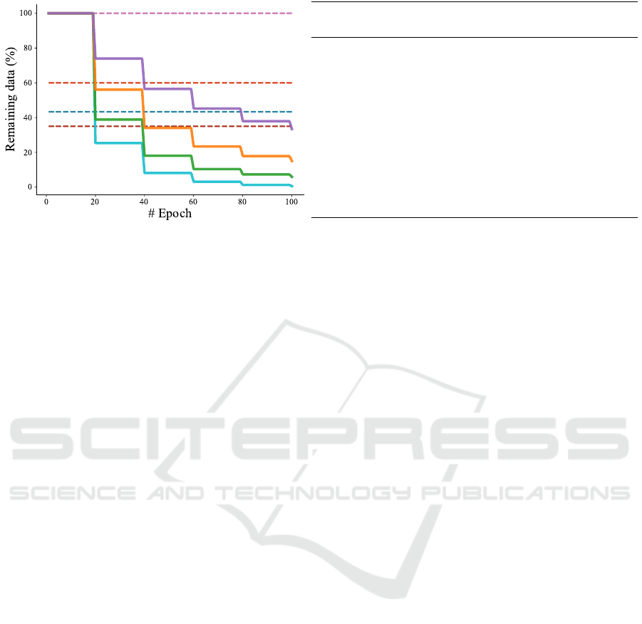
Figure 3: Evaluation of the impact of the amount of data pruned during training on a MNIST classification task. The left
panel shows the evolution of the pruned data over time, while the right panel presents the final accuracy, the average training
set size during training and remaining data at the end of training, the total training time, and the computation time of pruning.
The figure compares a uniform sampling without data pruning, random pruning with 60%, 43%, and 35% of data pruned,
the method of (Yang et al., 2023) at the same pruning rates, and our approach using a dynamic reduction factor K. Results
indicate that pruning more data accelerates execution. Our online pruning method offers greater adaptability during training
while maintaining high accuracy and minimal difference between training time and total execution time.
are seen multiple times within each epoch to match
the total step count.
Weight Stability. Updating the persistent per-
sample importance q directly sometime leads to a sud-
den decrease of accuracy during training. To make the
training process more stable, we update q by linearly
interpolating the importance at the previous and cur-
rent steps:
q(x) = α · q
prev
(x) + (1 − α) · q(x) (8)
where α is a constant for all data samples. In prac-
tice, we use α ∈ {0.0, 0.1, 0.2,0.3} as it gives the
best trade-off between importance update and stabil-
ity. This can be seen as a momentum evolution of the
per-sample importance to avoid high variation. Utiliz-
ing an exponential moving average to update the im-
portance metric prevents the incorporation of outlier
values. This is particularly beneficial in noisy setups,
like situations with a high number of class or a low
total number of data. Details on the chosen α values
can be found in Supplemental document.
7.2 Results
In Table 1, we compare Uniform sampling, Loss-
based importance sampling, the method from
(Katharopoulos and Fleuret, 2018) and their weights
in our algorithm, the approach from (Santiago et al.,
2021), and our method with both importance sam-
pling and data pruning. The table reports the cross-
entropy loss and classification accuracy for three
tasks: point cloud classification, CIFAR-100, and
Tiny-ImageNet. Results are shown for both an equal
number of steps and equal runtime. The best results
are highlighted in bold, with the second-best under-
lined. Across all three tasks, our method consis-
tently achieves the best performance in both scenar-
ios. Even in cases where importance sampling offers
minimal improvement, our approach proves more ro-
bust than DLIS and LOW, avoiding significant under-
performance in challenging situations. In the Tiny-
ImageNet experiment, although data pruning results
in a slight drop in accuracy, the outcome aligns with
the observations from (Yang et al., 2023), where prun-
ing can leads to a small reduction in generalization.
Additional results on other datasets can be found in
Supplemental document.
Figure 4 illustrates the results of a regression task
on an image using a SIREN network to learns the
mapping between 2D pixel coordinates and the cor-
responding RGB color. The left panel shows the
loss evolution for all methods, while the right panel
presents the error maps at final steps, along with a
zoomed-in region for Uniform sampling, DLIS, our
method with importance sampling, and our method
combining importance sampling and data pruning.
Our method, which incorporates importance sampling
and data pruning, provides the best loss reduction per-
formance. The error map reveals fewer errors, with
less yellow tones and finer details in the zoomed re-
gion. This method effectively reduces error in high-
frequency regions by compensating in smoother re-
gions such as the background, leading to a more bal-
anced error distribution across the image. In com-
Online Importance Sampling for Stochastic Gradient Optimization
137

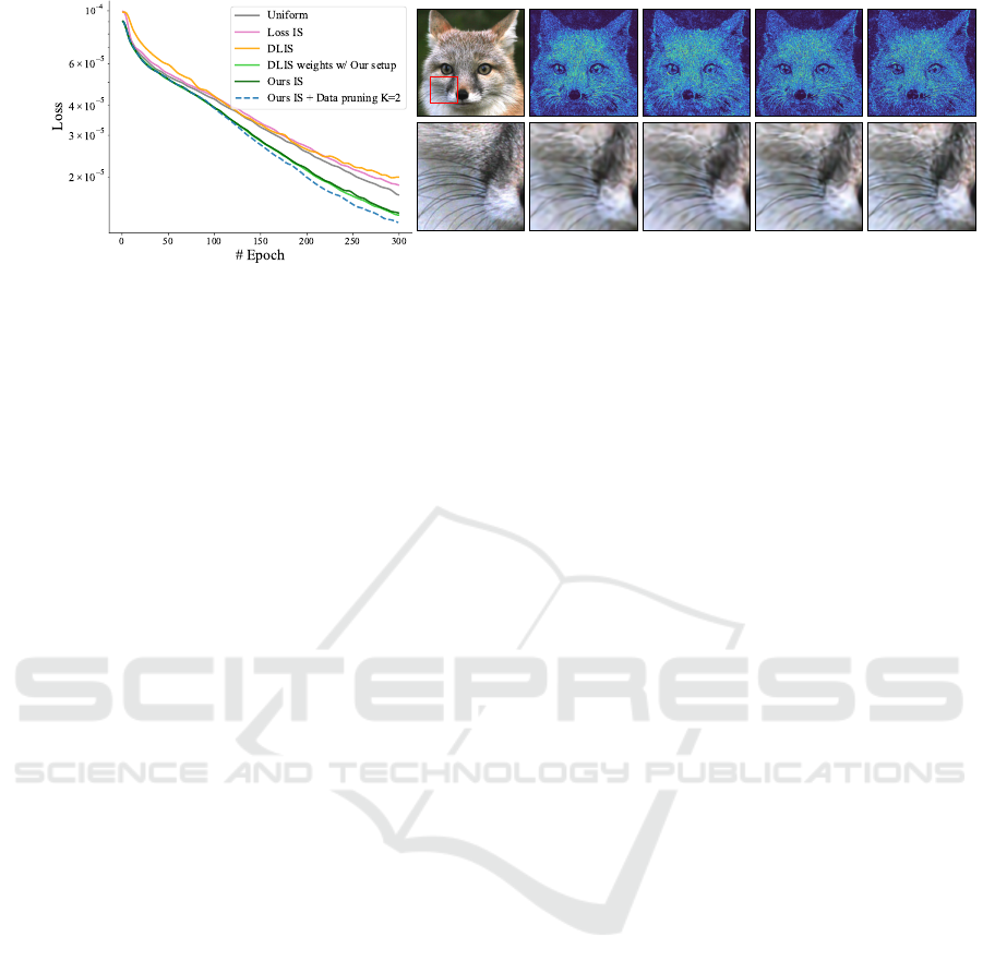
Reference Uniform DLIS Our IS
Our IS +
Data pruning (K=2)
Figure 4: Comparison at equal step for image 2D regression. The left side shows the convergence plot while the right display
the absolute error of the regression and a close-up view. Our method using data pruning achieves the lower error on this
problem while pruning 45% of the data during training. Our method using only importance sampling and DLIS with our
algorithm perform similarly, but DLIS with their full method perform worse than default optimization. In the images it is
visible that our method with pruning recovers the finest details of the fur and whiskers.
parison, DLIS produces similar results to our impor-
tance sampling when its weights are used with our
algorithm, but its full method is significantly out-
performed by Uniform sampling. This is evident in
the error map and the zoomed-in area, which display
more blurriness in DLIS results.
Figure 3 presents an ablation study of our online
pruning strategy on the MNIST classification task,
comparing random pruning, the method of (Yang
et al., 2023), and our adaptive approach. The left side
shows the evolution of the data used during training
across epochs, while the right side highlights final ac-
curacy, the average data used per epoch and the fi-
nal remaining data, the training time and time used
to compute the pruning. Our adaptive method starts
with the full dataset and prunes data every 20 epochs,
following Algorithm 2. As training progresses, the
amount of pruned data decreases, since many data
points begin to contribute redundant information. By
the end, only a reduced subset remains. In con-
trast, (Yang et al., 2023) prunes in one step at the
start using a pre-trained model, leading to faster train-
ing but lower quality results, not outperforming uni-
form sampling but providing generalization proper-
ties. Our approach adaptively removes data that no
longer adds value to the learning process. While ag-
gressive pruning (e.g., K = 1) risks overfitting and
reduced accuracy, more moderate pruning speeds up
training without sacrificing quality. The results show
that when minimal or no pruning is applied, the ad-
vantages diminish, reverting to a reliance on impor-
tance sampling alone. Overall, our adaptive pruning
efficiently reduces dataset size while preserving cru-
cial data throughout training.
Additional Experiments. Further comparisons,
similar to those in Table 1, across various datasets are
provided in Supplemental document. We also present
convergence curves at equal steps and equal time
intervals for Pointnet, CIFAR-10 (ViT (Dosovitskiy
et al., 2021)) and Tiny-ImageNet, demonstrating the
consistent improvements of our method throughout
the optimization process. These additional experi-
ments reinforce the effectiveness of our approach and
in particular benefit from a low computation method
at equal time.
Discussion. Both our and DLIS importance metrics
are highly correlated, but ours is simpler and more
efficient to evaluate. Even with a slightly better im-
portance sampling metric, most of the improvement
come from the memory-based algorithm instead of a
resampling one. The resulting algorithm gives bet-
ter performance at the same time and has more sta-
ble convergence. Our online data pruning method is
controlled by a pruning factor K, which dictates how
much data is removed at each step. While we kept K
constant in our experiments, it could be adjusted to
prevent overfitting. Pruned data could also be reintro-
duced later to check for overfitting by observing if its
importance increases after removal. This could help
detect reduced generalization without shrinking the
initial dataset, though we leave this for future work.
In theory, importance sampling can achieve error-
free estimation, when the sampling distribution is ex-
actly proportional to the integrand. However, that the-
oretical property holds only in the case where the esti-
mated quantity is scalar. In our case error-free estima-
tion is impossible even theoretically, because the es-
timated gradient is multi-dimensional, and there does
not exist a single (scalar) distribution that is propor-
tional to each dimension (i.e., parameter derivative).
To address this issue, (Sala
¨
un et al., 2024) explore the
use of multiple sampling distributions to further en-
hance gradient estimation. Their method builds upon
similar sampling metrics and algorithms to those pro-
ICPRAM 2025 - 14th International Conference on Pattern Recognition Applications and Methods
138

posed in this paper, demonstrating the potential for
improved accuracy through the use of diverse sam-
pling strategies.
Limitations. As the algorithm rely on past informa-
tion to drive a non-uniform sampling of data, it re-
quires seeing the same data multiple times. This cre-
ates a bottleneck for architectures that rely on pro-
gressive data streaming. More research is needed
to design importance sampling algorithms for data
streaming architectures, which is a promising future
direction. Non-uniform data sampling can also cre-
ate slower runtime execution. The samples selected
in a mini-batch are not laid out contiguously in mem-
ory leading to a slower loading. We believe a careful
implementation can mitigate this issue.
8 CONCLUSION
In conclusion, our work introduces an efficient sam-
pling strategy for machine learning optimization, that
can be use for importance sampling and data prun-
ing. This strategy, which relies on the gradient of the
loss and has minimal computational overhead, was
tested across various classification as well as regres-
sion tasks with promising results. Our work demon-
strates that by paying more attention to samples with
critical training information, we can speed up conver-
gence without adding complexity. We hope our find-
ings will encourage further research into simpler and
more effective sampling strategies for machine learn-
ing.
REFERENCES
Alain, G., Lamb, A., Sankar, C., Courville, A., and Bengio,
Y. (2015). Variance reduction in sgd by distributed im-
portance sampling. arXiv preprint arXiv:1511.06481.
Bordes, A., Ertekin, S., Weston, J., and Bottou, L. (2005).
Fast kernel classifiers with online and active learning.
Journal of Machine Learning Research, 6(54):1579–
1619.
Coleman, C., Yeh, C., Mussmann, S., Mirzasoleiman, B.,
Bailis, P., Liang, P., Leskovec, J., and Zaharia, M.
(2020). Selection via proxy: Efficient data selection
for deep learning. In International Conference on
Learning Representations.
Dong, C., Jin, X., Gao, W., Wang, Y., Zhang, H., Wu, X.,
Yang, J., and Liu, X. (2021). One backward from
ten forward, subsampling for large-scale deep learn-
ing. arXiv preprint arXiv:2104.13114.
Dosovitskiy, A., Beyer, L., Kolesnikov, A., Weissenborn,
D., Zhai, X., Unterthiner, T., Dehghani, M., Minderer,
M., Heigold, G., Gelly, S., Uszkoreit, J., and Houlsby,
N. (2021). An image is worth 16x16 words: Trans-
formers for image recognition at scale. In Interna-
tional Conference on Learning Representations.
Faghri, F., Duvenaud, D., Fleet, D. J., and Ba, J. (2020).
A study of gradient variance in deep learning. arXiv
preprint arXiv:2007.04532.
Gower, R. M., Loizou, N., Qian, X., Sailanbayev, A.,
Shulgin, E., and Richt
´
arik, P. (2019). SGD: Gen-
eral analysis and improved rates. In Chaudhuri, K.
and Salakhutdinov, R., editors, Proceedings of the
36th International Conference on Machine Learning,
volume 97 of Proceedings of Machine Learning Re-
search, pages 5200–5209. PMLR.
Gower, R. M., Schmidt, M., Bach, F., and Richt
´
arik, P.
(2020). Variance-reduced methods for machine learn-
ing. Proceedings of the IEEE, 108(11):1968–1983.
Hanchi, A. E., Stephens, D., and Maddison, C. (2022).
Stochastic reweighted gradient descent. In Chaudhuri,
K., Jegelka, S., Song, L., Szepesvari, C., Niu, G., and
Sabato, S., editors, Proceedings of the 39th Interna-
tional Conference on Machine Learning, volume 162
of Proceedings of Machine Learning Research, pages
8359–8374. PMLR.
Har-Peled, S. and Kushal, A. (2005). Smaller coresets
for k-median and k-means clustering. In Proceedings
of the Twenty-First Annual Symposium on Computa-
tional Geometry, SCG ’05, page 126–134, New York,
NY, USA. Association for Computing Machinery.
Horace He, R. Z. (2021). functorch: Jax-like composable
function transforms for pytorch. https://github.com/
pytorch/functorch.
Johnson, R. and Zhang, T. (2013). Accelerating stochastic
gradient descent using predictive variance reduction.
Advances in neural information processing systems,
26.
Katharopoulos, A. and Fleuret, F. (2017). Biased im-
portance sampling for deep neural network training.
ArXiv, abs/1706.00043.
Katharopoulos, A. and Fleuret, F. (2018). Not all sam-
ples are created equal: Deep learning with importance
sampling. In Dy, J. and Krause, A., editors, Pro-
ceedings of the 35th International Conference on Ma-
chine Learning, volume 80 of Proceedings of Machine
Learning Research, pages 2525–2534. PMLR.
Krizhevsky, A., Hinton, G., et al. (2009). Learning multiple
layers of features from tiny images.
Le, Y. and Yang, X. (2015). Tiny imagenet visual recogni-
tion challenge. CS 231N, 7(7):3.
Loshchilov, I. and Hutter, F. (2015). Online batch selection
for faster training of neural networks. arXiv preprint
arXiv:1511.06343.
Needell, D., Ward, R., and Srebro, N. (2014). Stochastic
gradient descent, weighted sampling, and the random-
ized kaczmarz algorithm. In Ghahramani, Z., Welling,
M., Cortes, C., Lawrence, N., and Weinberger, K., ed-
itors, Advances in Neural Information Processing Sys-
tems, volume 27. Curran Associates, Inc.
Nilsback, M.-E. and Zisserman, A. (2008). Automated
flower classification over a large number of classes.
Online Importance Sampling for Stochastic Gradient Optimization
139

In 2008 Sixth Indian conference on computer vision,
graphics & image processing, pages 722–729. IEEE.
Paul, M., Ganguli, S., and Dziugaite, G. K. (2021). Deep
learning on a data diet: Finding important examples
early in training. Advances in neural information pro-
cessing systems, 34:20596–20607.
Qi, C. R., Su, H., Mo, K., and Guibas, L. J. (2017). Point-
net: Deep learning on point sets for 3d classification
and segmentation. In Proceedings of the IEEE con-
ference on computer vision and pattern recognition,
pages 652–660.
Qin, Z., Wang, K., Zheng, Z., Gu, J., Peng, X., Xu, Z.,
Zhou, D., Shang, L., Sun, B., Xie, X., and You, Y.
(2023). Infobatch: Lossless training speed up by un-
biased dynamic data pruning.
Sala
¨
un, C., Huang, X., Georgiev, I., Mitra, N. J., and
Singh, G. (2024). Multiple importance sampling
for stochastic gradient estimation. arXiv preprint
arXiv:2407.15525.
Santiago, C., Barata, C., Sasdelli, M., Carneiro, G., and
Nascimento, J. C. (2021). Low: Training deep neural
networks by learning optimal sample weights. Pattern
Recognition, 110:107585.
Schaul, T., Quan, J., Antonoglou, I., and Silver, D.
(2015). Prioritized experience replay. arXiv preprint
arXiv:1511.05952.
Sitzmann, V., Martel, J., Bergman, A., Lindell, D., and Wet-
zstein, G. (2020). Implicit neural representations with
periodic activation functions. Advances in neural in-
formation processing systems, 33:7462–7473.
Toneva, M., Sordoni, A., des Combes, R. T., Trischler, A.,
Bengio, Y., and Gordon, G. J. (2019). An empirical
study of example forgetting during deep neural net-
work learning. In International Conference on Learn-
ing Representations.
Vandenberghe, L. (2010). The cvxopt linear and quadratic
cone program solvers. Online: http://cvxopt.
org/documentation/coneprog. pdf.
Wang, L., Yang, Y., Min, R., and Chakradhar, S. (2017).
Accelerating deep neural network training with incon-
sistent stochastic gradient descent. Neural Networks,
93:219–229.
Yang, S., Xie, Z., Peng, H., Xu, M., Sun, M., and Li, P.
(2023). Dataset pruning: Reducing training data by
examining generalization influence. In The Eleventh
International Conference on Learning Representa-
tions.
Zhang, C., Kjellstrom, H., and Mandt, S. (2017). Determi-
nantal point processes for mini-batch diversification.
arXiv preprint arXiv:1705.00607.
Zhang, C.,
¨
Oztireli, C., Mandt, S., and Salvi, G. (2019).
Active mini-batch sampling using repulsive point pro-
cesses. In Proceedings of the AAAI conference on Ar-
tificial Intelligence, volume 33, pages 5741–5748.
Zhang, M., Dong, C., Fu, J., Zhou, T., Liang, J., Liu,
J., Liu, B., Momma, M., Wang, B., Gao, Y., et al.
(2023). Adaselection: Accelerating deep learning
training through data subsampling. arXiv preprint
arXiv:2306.10728.
Zhao, P. and Zhang, T. (2015). Stochastic optimization with
importance sampling for regularized loss minimiza-
tion. In Bach, F. and Blei, D., editors, Proceedings of
the 32nd International Conference on Machine Learn-
ing, volume 37 of Proceedings of Machine Learning
Research, pages 1–9, Lille, France. PMLR.
ICPRAM 2025 - 14th International Conference on Pattern Recognition Applications and Methods
140