Optimization of Link Conﬁguration for Satellite Communication Using

Reinforcement Learning

Tobias Rohe

1 a

, Michael K

olle

1 b

, Jan Matheis

, R

udiger H

opﬂ

, Leo S

unkel

1 c

and Claudia Linnhoff-Popien

1 d

Mobile and Distributed Systems Group, LMU Munich, Germany

Airbus Defence and Space, Germany

ﬁ

Keywords:

Satellite Communication, Optimization, Link Conﬁguration, PPO Algorithm, Reinforcement Learning.

Abstract:

Satellite communication is a key technology in our modern connected world. With increasingly complex

hardware, one challenge is to efﬁciently conﬁgure links (connections) on a satellite transponder. Planning an

optimal link conﬁguration is extremely complex and depends on many parameters and metrics. The optimal

use of the limited resources, bandwidth and power of the transponder is crucial. Such an optimization problem

can be approximated using metaheuristic methods such as simulated annealing, but recent research results also

show that reinforcement learning can achieve comparable or even better performance in optimization methods.

However, there have not yet been any studies on link conﬁguration on satellite transponders. In order to close

this research gap, a transponder environment was developed as part of this work. For this environment, the

performance of the reinforcement learning algorithm PPO was compared with the metaheuristic simulated

annealing in two experiments. The results show that Simulated Annealing delivers better results for this static

problem than the PPO algorithm, however, the research in turn also underlines the potential of reinforcement

learning for optimization problems.

1 INTRODUCTION

In today’s world, satellite communication is a piv-

otal technology, utilized across a broad spectrum of

modern applications. While terrestrial communica-

tion systems depend on conventional infrastructure

that is often vulnerable to disruptions, satellite com-

munication has consistently demonstrated high reli-

ability. This reliability becomes especially crucial

in scenarios such as natural disasters, where large-

scale power outages often occur. In such cases, satel-

lite systems are vital for maintaining communication

channels .To further enhance the reliability and efﬁ-

ciency of satellite communication, reducing disrup-

tion, and optimize bandwidth usage, artiﬁcial intelli-

gence (AI) is increasingly being employed (V

azquez

et al., 2020).

A critical factor in the performance of satellite

communication networks is determining the optimal

https://orcid.org/0009-0003-3283-0586

https://orcid.org/0000-0002-8472-9944

https://orcid.org/0009-0001-3338-7681

https://orcid.org/0000-0001-6284-9286

link conﬁguration of the satellite transponder — an

inherently complex optimization problem. The opti-

mal conﬁguration of these links changes dynamically

as links are terminated or added. This dynamic na-

ture introduces the potential of reinforcement learning

(RL) as a method to optimize the link conﬁguration.

By leveraging learned metrics and the ability to

generalize, a RL approach could offer faster and su-

perior outcomes compared to traditional metaheuris-

tic approaches. In this paper, we model a satellite

transponder environment and illustrate how a mean-

ingful action and observation space can be deﬁned for

this purpose. Since modeling the dynamic aspects of

this problem exceeds the scope of this work, we have

chosen a static approach. In this context, static refers

to ﬁnding the best possible link conﬁguration for a

restricted number of links with predetermined param-

eter conﬁgurations. Building upon previous research,

where RL has achieved equal or better results than

metaheuristics for static optimization problems (Klar,

Glatt, and Aurich, 2023), we extend this investigation

to the speciﬁc optimization problem of link conﬁgu-

ration in satellite transponders.

The remainder of the paper is structured as fol-

704

Rohe, T., Kölle, M., Matheis, J., Höpﬂ, R., Sünkel, L. and Linnhoff-Popien, C.

Optimization of Link Conﬁguration for Satellite Communication Using Reinforcement Learning.

DOI: 10.5220/0013313000003890

Paper published under CC license (CC BY-NC-ND 4.0)

In Proceedings of the 17th International Conference on Agents and Artiﬁcial Intelligence (ICAART 2025) - Volume 2, pages 704-713

ISBN: 978-989-758-737-5; ISSN: 2184-433X

lows: Section 2 provides an overview of the back-

ground relevant to the study, followed by a discussion

of related work in Section 3. In Section 4, we present

our proposed approach for optimizing the link con-

ﬁguration. The experimental setup is detailed in Sec-

tion 5, and the results of the experiments are discussed

in Section 6. Finally, Section 7 concludes the paper

and outlines potential directions for future research.

2 BACKGROUND

2.1 Reinforcement Learning

Machine learning is a subﬁeld of artiﬁcial intelli-

gence, which can be further broken down into three

categories: supervised learning, unsupervised learn-

ing, and reinforcement learning (RL). RL is particu-

larly well-suited for addressing sequential decision-

making problems, such as those encountered in chess

or in the game AlphaGo (Deliu, 2023), where signif-

icant successes were achieved in recent years (Silver

et al., 2018). In RL, an agent learns a policy π by in-

teracting with an environment through trial and error,

with the goal of making optimal decisions. The two

main components in RL are the environment and the

agent. The environment is often modeled as a sim-

ulation of the real world, as an agent interacting di-

rectly with the real environment may be infeasible,

too risky or too expensive (Prudencio, Maximo, and

Colombini, 2023).

The foundation of RL lies in the Markov Deci-

sion Process (MDP). In an MDP, the various states of

the environment are represented by states in the pro-

cess. At any given time t, the agent occupies a state

. From this state, the agent can select from various

actions to transition to other states. Thus, the system

consists of state-action pairs, or tuples (A

, S

). When

the agent selects an action A

and executes it in the

environment, the agent receives feedback. This feed-

back includes an evaluation of the performed action

in the form of a reward, and the new state S

t+1

of the

environment. The reward may be positive or negative,

representing either a beneﬁt or a penalty. The agent’s

objective is to maximize the accumulated reward, as

shown in Equation 1.

∗

= arg max

∑

t=0

· R(s

, a

)

(1)

A major challenge in ﬁnding the optimal policy

∗

is the balance between exploration and exploita-

tion. Exploration refers to the degree to which the

agent explores the environment for unknown states,

while exploitation refers to the degree to which the

agent applies its learned knowledge to achieve the

highest possible reward. At the start of training, the

agent should focus more on exploring the environ-

ment, even if this means not always selecting the ac-

tion that yields the highest immediate reward (i.e.,

avoiding a greedy strategy). This approach allows the

agent to gain a more comprehensive understanding

of the environment and, ultimately, develop a better

policy. As the learning process progresses, the agent

should shift towards exploiting its knowledge more

and exploring less.

In RL, there is a distinction between model-based

and model-free approaches. In model-free RL, the

agent directly interacts with the environment and re-

ceives feedback. The environment may be a real-

world environment or a simulation. In contrast, in

model-based RL, the agent also interacts with the en-

vironment, but it can update its policy using a model

of the environment. In addition to standard RL, there

exists an advanced method called deep reinforcement

learning (deep RL). In deep RL, neural networks

are used to approximate the value function ˆv(s;θ) or

ˆq(s, a;θ) of the policy π(a | s; θ) or the model. The

parameter θ represents the weights of the neural net-

work. The use of neural networks enables the learn-

ing of complex tasks. During training, the connec-

tions between neurons, also called nodes, are dynam-

ically adjusted (weighted) to improve the quality of

the function approximation.

3 RELATED WORK

Metaheuristics are commonly applied to optimization

problems and frequently yield efﬁcient near-optimal

solutions in complex environments. A promising

alternative to these traditional approaches are RL-

algorithms, whose potential in the context of opti-

mization problems has already been scientiﬁcally ex-

plored (T. Zhang, Banitalebi-Dehkordi, and Y. Zhang,

2022; Ardon, 2022; Li et al., 2021). Studies such

as (Klar, Glatt, and Aurich, 2023) and (Mazyavk-

ina et al., 2021) demonstrate that RL-algorithms can

achieve results similar to or even superior to those ob-

tained by standard metaheuristics. This applies to a

variety of optimization problems, including the Trav-

eling Salesman Problem (TSP) (Bello et al., 2016),

the Maximum Cut (Max-Cut) problem, the Minimum

Vertex Cover (MVC) problem, and the Bin Packing

Problem (BPP) (Mazyavkina et al., 2021).

While the work by (Klar, Glatt, and Aurich, 2023)

does not focus on the arrangement of links on a

transponder, it focuses on the planning of factory

Optimization of Link Conﬁguration for Satellite Communication Using Reinforcement Learning

705

layouts, which is also a static optimization problem.

This study compares a RL-based approach with a

metaheuristic approach and examines which method

proves more effective. The research highlights RL’s

capability to learn problem-speciﬁc application sce-

narios, making it an intriguing alternative to conven-

tional methods. Given the uniqueness of each prob-

lem and the limited amount of scientiﬁc research on

this speciﬁc topic, individual consideration and anal-

ysis of each problem type are essential, which is also

goal of this research.

4 APPROACH

4.1 System Description

In satellite communication, ground stations are re-

sponsible for sending and receiving data. The data

is transmitted from the sending ground station to the

satellite via communication links, also referred to as

links or carriers, and then relayed from the satellite to

the receiving ground station via another link. On the

satellite itself, the links pass through chains of devices

known as transponders. Incoming signals are received

by an antenna on the satellite, ampliﬁed, converted in

frequency, and retransmitted through the antenna. A

transponder is a component within a satellite that re-

ceives signals transmitted from a ground station, am-

pliﬁes them with a speciﬁc ampliﬁcation factor using

the available power, changes their frequency to avoid

interference, and then retransmits the signals back to

Earth. This process enables the efﬁcient transmission

of information across vast distances in space. Figure

1 illustrates the path of the links as they move from

one ground station through the satellite’s transponder

to another ground station, facilitating data transmis-

sion.

However, each transponder has limited resources

in terms of bandwidth and power. It is crucial that the

links are conﬁgured to consume as few resources as

possible. A link is characterized by several parame-

ters, such as data rate, MOD-FEC combination (Mod-

ulation and Forward Error Correction), bandwidth,

and EIRP (Effective Isotropic Radiated Power). To

ensure the data is transmitted with sufﬁcient quality,

a minimum performance level must be maintained for

each link. The challenge lies in selecting the opti-

mal parameters for each link so that they use the least

possible resources on the transponder while maintain-

ing the required communication quality. This task is

further complicated because the bandwidth is a func-

tion of various other parameters. In the scenario con-

sidered here, a ﬁxed number of links are established

Figure 1: Illustration of Satellite Communication.

through which data is transmitted. Once the transmis-

sion is complete, all links are simultaneously taken

down.

4.2 Systemparameters

The following section outlines the process of estab-

lishing a satellite connection. To set up a link from a

ground station to a satellite, various parameters must

be carefully combined. The choice of these param-

eters determines how efﬁciently the links can be ar-

ranged on the satellite transponder, minimizing the

consumption of transponder resources, speciﬁcally

EIRP and bandwidth.

One key parameter is the EIRP, which represents

the power used to establish the link. Each link re-

quires a certain EIRP to ensure that the transmitted

data arrives with the desired quality. The necessary

EIRP depends on the data rate to be transmitted. The

data rate, typically measured in bits per second (bps),

indicates how much data can be transmitted per unit

of time and plays a crucial role in determining the re-

quired bandwidth.

The MOD-FEC combination is another essential

parameter. Modulation (MOD) is the process of con-

verting data into an electrical signal (electromagnetic

wave) for transmission, where characteristics of the

wave—such as amplitude, frequency, or phase—are

adjusted to encode the data. Forward Error Correction

(FEC) enables error detection and correction without

the need for retransmission, by adding correction in-

formation. The combination of modulation and FEC

greatly inﬂuences transmission efﬁciency, especially

in environments where interference is likely. Vari-

ous valid MOD-FEC combinations are available for

the transmission of a link, typically determined by the

hardware in use.

ICAART 2025 - 17th International Conference on Agents and Artiﬁcial Intelligence

706

Another important parameter is bandwidth, which

describes the ability of a communication channel or

transmission medium to transmit data over a speciﬁed

time period. Measured in Hertz (Hz), bandwidth di-

rectly inﬂuences transmission speed. In satellite com-

munication, bandwidth refers to the frequency range

over which a signal is transmitted. Both the data rate

and the MOD-FEC combination inﬂuence the deter-

mination of the bandwidth. To compute the band-

width, several parameters are required: FEC, MOD,

OH factor, RS factor, overhead, spacing factor, roll-

out factor, and the data rate. To simplify the model

of the environment, ﬁxed values were assigned to the

OH factor, RS factor, overhead, spacing factor, and

rollout factor. These parameters do not play a role in

the subsequent experiment but were included in the

calculation for the sake of completeness.

Calculating the bandwidth of a link involves three

steps. First, the transmission rate

UR is calculated by

multiplying the parameters data rate, OH factor, RS

factor, and FEC. This is shown in Equation 2.

UR = data rate ∗ OHFactor ∗ RSFactor ∗ FEC (2)

The transmission rate is then multiplied by the

MOD, resulting in the symbol rate (SR).

SR =

UR ∗ MOD (3)

Finally, the SR is multiplied by the Rollout Factor

and the Spacing Factor to obtain the bandwidth of a

link.

Bandwidth = SR ∗ Rollout Factor ∗ Spacing Factor

(4)

The last important parameter is the center fre-

quency, which determines the position of the links on

the transponder.

Link conﬁguration is usually carried out manually

with the support of software applications. However,

this is not an optimal procedure, as the ideal solution

is rarely found and therefore does not save resources.

In addition, the link conﬁguration has to be calculated

manually each time.

4.3 Action and Observation Space

In RL, the action space represents the set of all pos-

sible actions that an agent can perform within an en-

vironment. The agent responds to received observa-

tions by choosing an action. To analyze how different

action spaces affect performance, two distinct action

spaces were deﬁned.

The ﬁrst action space (Action Space 1) was de-

ﬁned using a nested dictionary from the Gymnasium

framework (gymnasium.spaces.Dict). This dictionary

contains three sub-dictionaries, each representing a

link. Each link dictionary includes the parameters

MOD-FEC combination, center frequency, and EIRP.

Both EIRP and center frequency are continuous val-

ues, so a ﬂoat value between 0 and 1 is selected at

each step within the environment. The MOD-FEC

combination, however, is a discrete value. A distinc-

tive feature of Action Space 1 is that all parameters

can be selected for any link at each step, allowing the

parameters to be reset at every action.

The second action space (Action Space 2) adopts

a different approach. Similar to Action Space 1, the

number of links is ﬁxed at exactly three. However,

the action space is represented as a 4-tuple (link, pa-

rameter, continuous, discrete). In this setup, a spe-

ciﬁc parameter is chosen for a link, and the value of

that parameter is modiﬁed. As with Action Space

1, EIRP and center frequency are continuous values,

while the MOD-FEC combination is represented by

discrete values.

The observation space in RL represents the set of

all possible states or information transmitted from the

environment to the agent. It contains all the neces-

sary information to reconstruct the current state of the

environment, including details about the link conﬁgu-

rations on the transponder. For each link, the observa-

tion space includes the parameters: center frequency,

EIRP, MOD-FEC combination, and Link Bandwidth

Percentage. The Link Bandwidth Percentage repre-

sents the portion of the transponder’s bandwidth allo-

cated to a particular link. This is calculated by divid-

ing the bandwidth of the link by the total transponder

bandwidth. The observation space remains consistent

for both Action Space 1 and Action Space 2.

4.4 Simpliﬁcations

In the experiments conducted, the task was simpliﬁed

in several aspects to facilitate the learning process.

Speciﬁcally, the transponder environment was simpli-

ﬁed. For instance, the possible MOD-FEC combina-

tions were restricted, and the modeling of the links in

the frequency domain was simpliﬁed, excluding the

interference of electromagnetic waves (links) which

normally affect communication quality.

Additionally, simpliﬁcations were made regarding

the inherently dynamic nature of the problem. Cur-

rently, a Proximal Policy Optimization (PPO) model

can only be trained for a ﬁxed number of links deﬁned

prior to training, which represents a static rather than

dynamic scenario. In our experiments, a PPO model

was trained exclusively for three links, and dynamic

changes — such as the addition or termination of links

Optimization of Link Conﬁguration for Satellite Communication Using Reinforcement Learning

707

— were not accounted for. The current environment

model is conﬁgured so that each link can be assigned

one of three possible MOD-FEC combinations, and

the data rate for each link is set to a uniform value.

Future iterations of the model will progressively

address these simpliﬁcations to handle the more com-

plex tasks encountered in real-world scenarios.

5 EXPERIMENTAL SETUP

Two experiments were conducted, differing only in

the conﬁguration of the RL model. The PPO al-

gorithm was utilized in both models, with the only

distinction being the action space, as explained in

Chapter 4.3. For both experiments, Python (version

3.8.10), PyTorch (version 1.13.1), Gymnasium (ver-

sion 0.28.1), and Ray RLlib (version 0.0.1) were used.

5.1 PPO Algorithm

The PPO model serves as the baseline against which

the Random Action and Simulated Annealing base-

lines are compared in terms of performance. A neu-

ral network was used to implement the PPO, tasked

with calculating the policy parameters. The neural

network topology consisted of the observation space

as the input layer, followed by two hidden layers with

256 neurons each, and the action space as the output

layer. The learning rate for the PPO model was op-

timized, with further details provided in the section

”Training Process”. The hyperparameters are shown

in Table 1.

Table 1: PPO Algorithm Hyperparameter Conﬁguration.

Parameter Datatype Value

Discount Factor Float 0.99

Batch Size Integer 2000

Clipping Range Float 0.3

GAE Lambda Float 1.0

Entropy coeff Float 0.0

Number of SGD Integer 30

Minibatchsize Integer 128

5.2 Random Action Strategy

The na

ıve random action strategy, which is compared

with the PPO, consists of choosing actions purely at

random. We deﬁne a fundamental learning success

here if the PPO model achieves better results than the

random action model.

5.3 Simulated Annealing

Simulated annealing follows a structured process: Ini-

tially, the algorithm is provided with a randomly gen-

erated action. This action is evaluated by the cost

function, which in this case is represented by the step

function of the environment. The corresponding re-

ward for the action is calculated. Next, the neighbor

function generates a new action. If the reward of the

new action is better than that of the previous action,

it is accepted as the new action. However, if the re-

ward is lower, the new action is not immediately dis-

carded. An additional mechanism, known as temper-

ature, plays a key role in determining the probability

of selecting a worse action as the new action.

At the beginning of the algorithm, the temperature

is high, leading to a higher probability of choosing a

worse action. This facilitates broader exploration in

the search for the global optimum. As the algorithm

progresses, the temperature decreases gradually. As

the temperature lowers, the probability of accepting

a worse action diminishes, leading to a more focused

search for the local optimum and enabling ﬁne-tuning

of the solution.

Table 2: Simulated Annealing Hyperparameter Conﬁgura-

tion.

Parameter Datatype Value

Tries Integer 0.99

Max Step Integer 2000

T min Integer 0

T max Integer 100

Damping Float 0.0

Alpha Float 30

5.4 Metrics

The metric for evaluating link conﬁguration on the

satellite transponder is the total reward, which reﬂects

the learning behavior of the model. This total re-

ward comprises eight metrics, each linked to speciﬁc

conditions in the link conﬁguration. The metrics are

detailed below along with their calculation methods.

They are categorized into Links Reward (LR) and

Transponder Reward (TR), contributing 70% (0.7)

and 30% (0.3) to the total reward, respectively. In-

dividual metrics can be weighted to emphasize more

challenging metrics (through the parameters ω, θ, φ,

µ, β, ε, ψ, ρ), potentially enhancing policy learning

for the PPO agent. However, the impact of different

weightings was not explored in this study.

Links reward metrics include Overlap Reward,

On Transponder Reward, PEB Reward, and Mar-

gin Reward, which pertain to each link individually.

ICAART 2025 - 17th International Conference on Agents and Artiﬁcial Intelligence

708

Since multiple links are typically conﬁgured on the

transponder, the link reward is divided by the num-

ber of links to represent the reward per link-weight

(RpL). This share, multiplied by the Individual Link

Reward for each link, contributes to the total reward

(see Equation 9). Metrics for each link are:

• Overlap Reward (OR): Checks if the selected link

does not overlap with other links in terms of band-

width. A reward of 1 is given if met; otherwise,

OR = RpL × ω × or (5)

• On Transponder Reward (OTR): Veriﬁes whether

the link’s bandwidth is fully on the transponder. If

met, the reward is 1; if not, 0.

OTR = RpL × θ ×tr (6)

• PEB Reward (PEBR): Assesses the appropriate-

ness of the power-to-bandwidth ratio for the link.

A reward of 1 is given if met; otherwise, 0.

PEBR = RpL × φ × pebr (7)

• Margin Reward (MR): Evaluates the EIRP of the

link. If it is below the minimum required for high-

quality transmission, no reward is given. If ex-

actly at the minimum, the reward is 1. If above,

the reward decreases as the EIRP exceeds the min-

imum.

MR = RpL × µ × mr (8)

Individual Link Reward =

∑

(OR + OTR + PEBR + MR)

(9)

TR metrics relate to all links or the system as a

whole, it includes:

• Bandwidth Reward (BR): Measures the ratio of

the sum of link bandwidths to the transponder

bandwidth. The PPO agent should learn that this

sum must not exceed the transponder bandwidth.

A reward of 1 is given if met; otherwise, 0.

BR = TR × β (10)

• EIRP Reward (ER) : Assesses the ratio of total

link EIRP to transponder EIRP. The PPO agent

should learn that the sum of link EIRPs must not

exceed the transponder EIRP to avoid overload-

ing. A reward of 1 is given if met; otherwise, 0.

ER = TR × ε (11)

• Packed Reward (PR):This metric measures the

utilization of overlapping frequency ranges for

links on the transponder. A reward is given based

on how well the overlapping frequencies are man-

aged, encouraging conﬁgurations that maximize

frequency usage without excessive interference.

PR = TR × ψ (12)

• Free Resource Reward (FRR): This metric evalu-

ates the amount of unused or free resources (e.g.,

bandwidth or power) on the transponder. It likely

rewards conﬁgurations that conserve resources,

promoting efﬁcient use of the transponder’s lim-

ited capabilities.

FRR = TR × ρ (13)

Transponder Reward =

∑

(BR + ER + PR + FRR)

(14)

5.5 Training Process

Before initiating the experiments, the learning rate

for the PPO was examined through a grid search.

For the ﬁrst experiment, the grid search included val-

ues of 1e − 3, 5e − 4, 1e − 4, 5e − 5, and 1e − 5.

Each learning rate was evaluated using three differ-

ent seeds. Across all runs, 2, 000, 000 steps were ex-

ecuted in the transponder environment, maintaining a

consistent batch size of 2, 000 for comparability. Each

episode consisted of 10 steps, serving as the termina-

tion criterion, resulting in a total of 200, 000 episodes.

The best performance was obtained with a learning

rate of 1e − 5. This learning rate was subsequently

used for Experiment 1.

A similar grid search was performed for the sec-

ond experiment, with learning rate values set at 1e−3,

1e−4, and 1e −5. Each learning rate was again tested

with three different seeds. For all runs, 1, 000, 000

steps were carried out in the transponder environment,

with a batch size of 2, 000. Episodes consisted of 100

steps. Also for Experiment 2, a learning rate of 1e −5

yielded the best performance.

6 RESULTS

6.1 Experiment 1

The objective of the ﬁrst experiment was to determine

an optimal link conﬁguration for three links within

the transponder environment, ensuring that the band-

width and EIRP resources of the satellite transponder

were conserved. To address this optimization prob-

lem, the three algorithms — PPO, Simulated Anneal-

ing, and Random Action — were implemented in the

transponder environment. The experiment aimed to

evaluate whether a trained PPO model could achieve

higher performance compared to the Simulated An-

nealing algorithm. Action Space 1 was used in the

environment for this experiment.

Optimization of Link Conﬁguration for Satellite Communication Using Reinforcement Learning

709

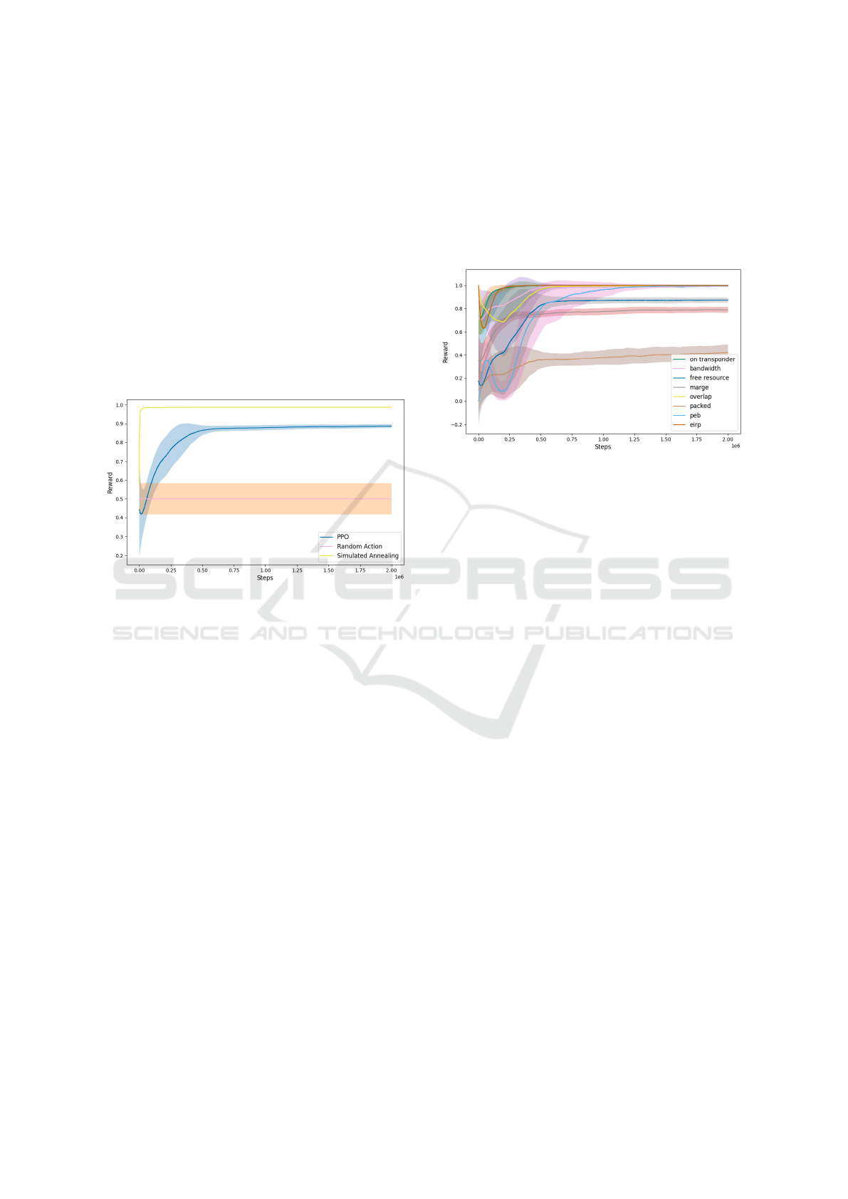
Figure 2 illustrates the training of the PPO model

over 2, 000, 000 steps, compared to the Simulated An-

nealing and Random Action baselines. Each PPO

episode consisted of 10 steps. To enhance visualiza-

tion, all curves were smoothed. Training for the PPO

model and the computation of the comparative base-

lines were conducted with ﬁve different seeds (0 to 4).

The ﬁgure presents the average performance across

these runs, including the standard deviation for each

algorithm. The maximum achievable value is 1. It

is noteworthy that only the PPO model was trained,

as neither the Simulated Annealing algorithm nor the

Random Action model can be trained. These base-

lines were plotted to provide a benchmark for assess-

ing the PPO’s performance.

Figure 2: Comparison PPO, Simulated Annealing and Ran-

dom Action. The x-axis represents the training steps; the

y-axis shows the achieved Reward.

Both the Simulated Annealing and Random Ac-

tion models were run for 2,000,000 steps. As ex-

pected, the Random Action model showed the lowest

performance, maintaining an average value of 0.496

across all steps. The PPO model started at a similar

value, which is typical as no policy has been learned

at the initial stage. The policy improved continu-

ously over the steps, as indicated by an increase in re-

ward, with most adjustments occurring within the ﬁrst

500, 000 steps. After this, the PPO curve gradually

converged to just below 0.9, indicating that an effec-

tive policy had been learned. The Simulated Anneal-

ing algorithm demonstrated the highest performance,

rapidly reaching a value just under 1 within the ﬁrst

20, 000 steps and converging toward 1 thereafter.

Figure 3 depicts the learning behavior of the PPO

model for the individual metrics that collectively con-

tribute to the total reward. These metrics represent

conditions that should be met, as explained in Sec-

tion 5.4. The On Transponder Reward, EIRP Reward,

Overlap Reward, PEB Reward, and Bandwidth Re-

ward metrics were effectively learned by the PPO,

each reaching the maximum value of 1. A second

group of metrics, including Packed Reward, Free Re-

source Reward, and Margin Reward, showed slower

learning progress and had not reached their maxi-

mum values by the end of training. The slight upward

trend of these curves at the end of training suggests

that additional training could further improve the PPO

model’s performance.

Figure 3: Development of Rewards under the PPO algo-

rithm Training. The learning behavior of the PPO with re-

gards to the various reward components is illustrated. The

steps are printed on the x-axis, the reward on the y-axis.

To evaluate the performance of the PPO model

ﬁnally, the trained PPO model, the Simulated An-

nealing model, and the Random Action model were

applied to unseen observations, referred to as infer-

ence. Unlike the training phase, the PPO does not re-

ﬁne its policy during this step but applies the learned

policy. Five seeds (0–4) were used for evaluation.

In each run, ﬁve different random observations were

generated for the conﬁguration of three links. Dur-

ing an episode, the PPO model’s task was to conﬁg-

ure the links optimally. Each episode consisted of 10

steps, with the PPO applying its policy learned over

2, 000, 000 training steps.

The Random Action model achieved an average

value of 0.496. The Simulated Annealing model

reached a value of 0.988, requiring 2, 000, 000 steps

to do so. However, as shown in Figure 2, only

20, 000 steps would have been sufﬁcient, as the Sim-

ulated Annealing model’s performance converged to-

ward 1 from that point onward. Detailed results of

the ﬁrst experiment are provided in Table 3. The

evaluation demonstrates that the Simulated Annealing

model achieved the best performance, with a value of

0.988. The PPO model also performed well, achiev-

ing a value of 0.875. It is noteworthy that the opti-

mization of the PPO model only considered the learn-

ing rate through a grid search, while other potentially

beneﬁcial hyperparameters were not explored.

ICAART 2025 - 17th International Conference on Agents and Artiﬁcial Intelligence

710

Table 3: Experiment 1: Inference.

Algorithmus Reward

PPO (Action Space 1) 0.875 ± 0.007

Simulated Annealing 0.988 ± 0.001

Random Action 0.496 ± 0.004

6.2 Experiment 2

Experiment 2 differs from Experiment 1 in that it uses

Action Space 2, deﬁned such that a parameter value

can be modiﬁed from a link in a single step. The pa-

rameters available for modiﬁcation include center fre-

quency, EIRP, and the MOD-FEC combination. As in

Experiment 1, PPO was compared with the Simulated

Annealing and Random Action baselines. The se-

lected learning rate for PPO was 1e−5, as this yielded

the best performance during the grid search for Action

Space 2.

Figure 4 illustrates the training process for Ex-

periment 2, where the PPO model was trained over

1, 000, 000 steps, with each episode comprising 100

steps. The Simulated Annealing and Random Ac-

tion baselines were also executed for 1, 000, 000 steps.

The graphs for Simulated Annealing and Random Ac-

tion are identical to those in Experiment 1. As shown,

the most signiﬁcant adjustments in PPO occur during

the ﬁrst 200, 000 training steps.

Figure 4: Comparison PPO, Simulated Annealing and Ran-

dom Action. The x-axis represents the training steps; the

y-axis shows the achieved Reward.

Subsequently, the PPO curve converges toward a

value of approximately 0.7, suggesting that the opti-

mization problem may be somewhat too complex for

the deﬁned Action Space 2. Given that the PPO curve

in Figure 4 continues to rise slowly, further training

could potentially enhance the PPO model’s perfor-

mance. However, the individual metrics contributing

to the Total Reward metric are less well-learned with

Action Space 2 compared to Action Space 1, as indi-

cated in Figure 5. The EIRP Reward is the only met-

ric fully learned, while the other metrics learn more

slowly or converge at different levels after brief train-

ing. The Figure suggests that extended training could

improve the total reward, although it remains uncer-

tain how much the PPO model can improve, given

that a signiﬁcant number of metrics are not effectively

learned by the policy.

Figure 5: Development of Rewards under the PPO algo-

rithm Training. The learning behavior of the PPO with re-

gards to the various reward components is illustrated. The

steps are printed on the x-axis, the reward on the y-axis.

Also for the second experiment, the models were

evaluated on unseen data. As in Experiment 1, the

Simulated Annealing algorithm achieved the best per-

formance. The PPO model reached a value of 0.786,

performing worse than the Simulated Annealing al-

gorithm. However, since the PPO model’s value was

notably higher than that of the Random Action model,

it can be inferred that the PPO model had effectively

learned.

The lower performance of the PPO model com-

pared to Experiment 1 could be attributed to the ac-

tion space implementation not sufﬁciently capturing

the complexity of the problem. As discussed, the re-

sults of Experiment 2 should be considered an ini-

tial assessment. Further improvements in perfor-

mance could be achieved by adjusting hyperparam-

eters, modifying the weighting of the action space

metrics, or employing reward shaping or curriculum

learning.

Table 4: Experiment 2: Inference.

Algorithmus Reward

PPO (Action Space 2) 0.786 ± 0.104

Simulated Annealing 0.988 ± 0.001

Random Action 0.496 ± 0.004

6.3 Interpretation

The results achieved with Action Space 1 are supe-

rior to those obtained with Action Space 2. One pos-

sible explanation for this is that, during training, the

Optimization of Link Conﬁguration for Satellite Communication Using Reinforcement Learning

711

randomly generated actions in Action Space 1 evenly

scan the action space. In contrast, with Action Space

2, certain regions are densely sampled while others

receive little to no sampling. Consequently, inference

using an Action Space 2 PPO model yields very good

results in well-sampled areas and signiﬁcantly poorer

results in sparsely sampled areas.

Another possible reason for the better perfor-

mance of Action Space 1 could be the simpler and

more direct relationship between the Action Space

and Observation Space, making it easier to learn. In

Action Space 1, there is a one-to-one correspondence

between the parameters in the Action Space and those

in the Observation Space. In Action Space 2, how-

ever, this mapping is more complex, complicating the

learning process.

7 CONCLUSION

Even today, the conﬁguration of connections in satel-

lite communication networks is often performed man-

ually. Given the increasing complexity of the hard-

ware used both in satellites and on the ground, the

application of AI in this domain is a logical progres-

sion. In this work, a transponder environment was de-

veloped for link conﬁguration on a satellite transpon-

der, and the potential utility of RL for solving a static

problem was investigated. Two experiments were

conducted, differing in their implementation of the

action space. In both, a PPO model was compared

to two baselines: Simulated Annealing and the Ran-

dom Action model. The results showed that in both

experiments, the Simulated Annealing metaheuristic

outperformed the PPO model. Since only the learning

rate was optimized for the PPO, further improvements

could be achieved through additional hyperparameter

tuning. Additionally, the weighting of the metrics was

not explored, which could be another factor for en-

hancing PPO performance.

It is likely that the performance gap between Sim-

ulated Annealing and PPO would widen as the static

problem becomes more complex and realistic. Sim-

ulated Annealing is speciﬁcally designed for efﬁcient

exploration of large search spaces, potentially demon-

strating even greater superiority over PPO in more

complex scenarios. Given the growing complexity of

this ﬁeld, continued research is essential to ﬁnd so-

lutions to this optimization problem. The environ-

ment must be reﬁned to better match real-world re-

quirements. For instance, only a single data rate was

used in this study, whereas in practice, this parameter

is continuous or must be represented in a rasterized

form. The mutual interference between links was ne-

glected and needs to be incorporated for practical ap-

plications. The restriction to exactly three links must

also be removed. An important next step is to transi-

tion from a static to a dynamic model, allowing each

link to have an active time period. The agent must

also evolve alongside the environment, with the neu-

ral network topology becoming more complex. A po-

tential strength of PPO could be its ability to handle

scenarios where links on the transponder are dynam-

ically added or terminated over time, leveraging its

capacity to learn policies that comprehend underlying

metrics. However, this potential requires further ex-

perimentation and comprehensive research.

Overall, these future steps present an opportunity

to enhance the developed model, align it with the

complexity of real-world environments, and validate

its practical applicability.

ACKNOWLEDGEMENTS

This paper was partially funded by the German Fed-

eral Ministry of Education and Research through the

funding program ”quantum technologies - from basic

research to market” (contract number: 13N16196).

Furthermore, this paper was also partially funded

by the German Federal Ministry for Economic Af-

fairs and Climate Action through the funding program

”Quantum Computing – Applications for the indus-

try” (contract number: 01MQ22008A).

REFERENCES

Ardon, L. (2022). “Reinforcement Learning to Solve NP-

hard Problems: an Application to the CVRP”. In: arXiv

preprint arXiv:2201.05393.

Bello, I. et al. (2016). “Neural combinatorial optimiza-

tion with reinforcement learning”. In: arXiv preprint

arXiv:1611.09940.

Deliu, N. (2023). “Reinforcement learning for sequential

decision making in population research”. In: Quality &

Quantity, pp. 1–24.

Klar, M., M. Glatt, and J. C. Aurich (2023). “Performance

comparison of reinforcement learning and metaheuris-

tics for factory layout planning”. In: CIRP Journal of

Manufacturing Science and Technology 45, pp. 10–25.

Li, K. et al. (2021). “Deep reinforcement learning for com-

binatorial optimization: Covering salesman problems”.

In: IEEE transactions on cybernetics 52.12, pp. 13142–

13155.

Mazyavkina, N. et al. (2021). “Reinforcement learning for

combinatorial optimization: A survey”. In: Computers

& Operations Research 134, p. 105400.

ICAART 2025 - 17th International Conference on Agents and Artiﬁcial Intelligence

712

Prudencio, R. F., M. R. Maximo, and E. L. Colom-

bini (2023). “A survey on ofﬂine reinforcement learn-

ing: Taxonomy, review, and open problems”. In: IEEE

Transactions on Neural Networks and Learning Sys-

tems.

Silver, D. et al. (2018). “A general reinforcement learn-

ing algorithm that masters chess, shogi, and Go through

self-play”. In: Science 362.6419, pp. 1140–1144.

azquez, M.

A. et al. (2020). “On the use of AI

for satellite communications”. In: arXiv preprint

arXiv:2007.10110.

Zhang, T., A. Banitalebi-Dehkordi, and Y. Zhang (2022).

“Deep reinforcement learning for exact combinatorial

optimization: Learning to branch”. In: 2022 26th In-

ternational Conference on Pattern Recognition (ICPR).

IEEE, pp. 3105–3111.

Optimization of Link Conﬁguration for Satellite Communication Using Reinforcement Learning

713