Can Bayesian Neural Networks Explicitly Model Input Uncertainty?

Matias Valdenegro-Toro

and Marco Zullich

Department of Artiﬁcial Intelligence, University of Groningen, Nijenborgh 9, 9747AG, Groningen, Netherlands

Keywords:

Uncertainty Estimation, Input Uncertainty, Feature Uncertainty.

Abstract:

Inputs to machine learning models can have associated noise or uncertainties, but they are often ignored and

not modelled. It is unknown if Bayesian Neural Networks and their approximations are able to consider un-

certainty in their inputs. In this paper we build a two input Bayesian Neural Network (mean and standard de-

viation) and evaluate its capabilities for input uncertainty estimation across different methods like Ensembles,

MC-Dropout, and Flipout. Our results indicate that only some uncertainty estimation methods for approximate

Bayesian NNs can model input uncertainty, in particular Ensembles and Flipout.

1 INTRODUCTION

In the last two decades, Neural Networks (NNs) have

become state-of-the-art applications in many differ-

ent domains, such as computer vision and natural

language processing. Despite this, these models are

known as being notoriously bad at modelling un-

certainty, especially when considering the frequen-

tist setting (Valdenegro-Toro, 2021a), in which ﬁxed

parameters are trained to minimize a loss function.

Indeed, while NNs for regression lack a direct way

to estimate uncertainty, Deep NNs for classiﬁcation

are often found to be extremely overconﬁdent in their

predictions (Guo et al., 2017), even when running

inference with random data (Nguyen et al., 2015).

Bayesian Neural Networks (BNNs), which consider

parameters as probability distributions, provide a nat-

ural way to produce uncertainty estimates, both in

the regression and in the classiﬁcation setting (Pa-

padopoulos et al., 2001). They have been proven

to be substantially better at producing more reliable

uncertainty estimates, albeit the quality depends on

the techniques which are used to approximate these

models (Ovadia et al., 2019). A model whose uncer-

tainty estimates are reliable is also called calibrated,

and one of the main metrics for calibration is called

the Expected Calibration Error (ECE) (Naeini et al.,

2015).

Uncertainty, in the context of Machine Learning,

is split in two categories (H

ullermeier and Waege-

man, 2021): (a) epistemic or model uncertainty, and

https://orcid.org/0000-0001-5793-9498

https://orcid.org/0000-0002-9920-9095

Figure 1: Sample of data from the Fashion-MNIST dataset

with Gaussian noise with increasing standard deviation (σ

in the ﬁgure) added. The ﬁrst row (σ = 0.0) represents the

original, unperturbed data. Natural data are often captured

by means of digital sensors, which are prone to be noisy

and can sporadically fail. Training NNs which can effec-

tively model input uncertainty, especially when the noise is

anomalously high, is important in having reliable predic-

tions, which can be discarded whenever the predictive un-

certainty of the model is too high.

(b) aleatoric or data uncertainty—here also called in-

put uncertainty. These two types of uncertainty are

usually implicitly modelled together in a single con-

cept, called predictive uncertainty, and the process of

recovering the epistemic and aleatoric components is

called uncertainty disentanglement (Valdenegro-Toro

and Mori, 2022). An effective modeling of aleatoric

and epistemic uncertainty by a machine learning

model is crucial whenever this model needs to (a) be

deployed in-the-wild, or (b) be used (in assisting) for

decision-making in safety-critical situations. In these

cases, it is paramount that model is well calibrated: if

it is presented with anomalous or unknown data—for

188

Valdenegro-Toro, M. and Zullich, M.

Can Bayesian Neural Networks Explicitly Model Input Uncertainty?.

DOI: 10.5220/0013313300003912

Paper published under CC license (CC BY-NC-ND 4.0)

In Proceedings of the 20th International Joint Conference on Computer Vision, Imaging and Computer Graphics Theory and Applications (VISIGRAPP 2025) - Volume 3: VISAPP, pages

188-199

ISBN: 978-989-758-728-3; ISSN: 2184-4321

Classical NN

σ = 0.0 σ = 0.5 σ = 1.0

σ = 1.5

σ = 2.0

DropoutDropConnect5 EnsemblesFlipoutDUQ

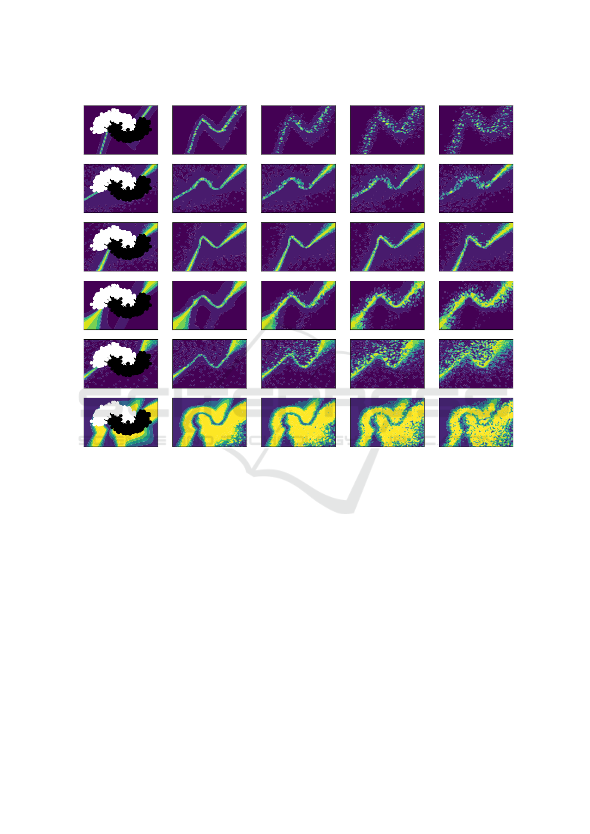
Figure 2: Comparison on the Two Moons dataset with training σ = 0.2, as the testing standard deviation is varied. Each

heatmap indicates predictive entropy (low blue to high yellow) and the ﬁrst column includes the training data points, With

larger test standard deviation, some UQ methods do not signiﬁcantly change their output uncertainty (DropConnect, Dropout,

DUQ), while Flipout and Ensembles do have signiﬁcant changes, indicating that they are able to model input uncertainty and

propagate it to the output.

which it effectively behaves randomly—we want this

reﬂected in the prediction uncertainty. In this sense, a

highly unconﬁdent prediction can be discarded a pri-

ori because it has a high chance of being inaccurate.

The digitization of natural data requires captur-

ing it with either manual measurements or sensors,

both procedures which are subjects to noise: this

represents aleatoric uncertainty; recapturing the data

within the same condition several times will lead to

different measurements. We can thus summarize each

data point as a mean data and the corresponding stan-

dard deviation.

In the present work, instead of letting the NNs im-

plicitly model predictive uncertainty, we provide the

input uncertainty as input, in addition to the mean

value of the data. We call these models two-input

NNs.

We provide our results on two small-scale clas-

siﬁcation tasks: the Two Moons toy example and

the Fashion-MNIST dataset (Xiao et al., 2017). We

train classical NNs and ﬁve approximate classes of

BNNs (MC-Dropout, MC-DropConnect, Ensembles,

Flipout, Direct Uncertainty Quantiﬁcation—DUQ)

on these tasks. We observe the behavior of the un-

certainty and ECE when different values of noise are

injected into the data and conclude that often these

models fail to correctly estimate input uncertainty.

The investigation of the quality of predictive un-

certainty estimates for machine learning models is a

long-studied subject and is usually associated with

Bayesian modeling (Roberts, 1965): given the fact

that these models output a probability distribution,

its deviation can be used as a natural estimate of un-

certainty. Deterministic NNs predict point estimates,

Can Bayesian Neural Networks Explicitly Model Input Uncertainty?

189

(a) σ = 0.0 (b) σ = 0.2 (c) σ = 0.4 (d) σ = 0.6 (e) σ = 0.8

Figure 3: The version of the Two Moons dataset (with 1000 data points) used in the present work, the two colors representing

the two categories. From left to right, we add an increasingly higher level of zero-mean Gaussian noise. The standard

deviation is denoted by σ.

thus they lack a natural expression of uncertainty, ex-

cept for the case of classiﬁcation, where the output—

after the application of the softmax function—is inter-

pretable as a probability distribution. Initial attempts

at computation of probability intervals on the out-

put of NNs include the usage of two-headed models

which output a mean prediction and the standard de-

viation (Nix and Weigend, 1994) and early-day BNNs

(MacKay, 1992). None of these attempts, though,

propose a direct modeling of data uncertainty.

Nonetheless, there are more recent efforts for

achieving this. (Wright, 1998) and (Wright, 1999)

use the Laplace approximation to train a BNN with

input uncertainty, but this is not a modern BNN and

it is only tested on simplistic regression settings.

(Tzelepis et al., 2017) introduce a variation of Support

Vector Machines which include a Gaussian noise for-

mulation for each data point, which is directly taken

into consideration in the hinge loss for determining

the separating hyperplane. (Rodrigues et al., 2023)

introduce the concept of two-input NNs by crafting

a simple toy classiﬁcation problem, showing how, by

providing more information as input to the models,

their NNs perform better than the regular, “single-

input” counterparts. (H

ullermeier, 2014), instead, fo-

cuses on producing fuzzy loss functions to utilize in

a deterministic setting. This allows to incorporate

input uncertainty in the empirical risk minimization

paradigm. All of these three works limit their investi-

gations to toy problems and, moreover, do not provide

insights into the evaluation of uncertainty estimates.

To the best of our knowledge, we are the ﬁrst to in-

vestigate the capability of modern BNNs to explicitly

model input uncertainty, by providing an analysis on

the quality of the uncertainty that these models pro-

duce. Our hypothesis is that models being presented

with aleatoric uncertainty as input will not be able to

effectively reﬂect it in the predictive uncertainty, ex-

hibiting high levels of conﬁdence even when the input

is anomalously noisy.

The contributions of this work are an evaluation

of the capability of BNNs to explicitly model uncer-

tainty in their inputs, we evaluate several uncertainty

estimation methods and approximate BNNs, and con-

clude that only Ensembles are—to a certain extent—

reliable when considering explicit uncertainty in its

input.

2 EVALUATING BAYESIAN

NEURAL NETWORKS

AGAINST INPUT

UNCERTAINTY

2.1 Datasets

We base our experiments on two datasets, the Two

Moons dataset and Fashion-MNIST.

Two Moons. Two Moons is a toy binary classiﬁcation

problem available in the Python library scikit-learn

(Kramer and Kramer, 2016). It is composed by a vari-

able number of 2d data points generated in forming

two interleaving half circles. Due to the ease of visu-

alization, it is often being used in research on uncer-

tainty estimation for visualizing the capability of the

models to produce reliable uncertainty values in and

around the domain of the dataset. Notice that, due to

its toy nature, this dataset only comes with a training

set, i.e., there are no validation or test splits. Some

examples of unperturbed and perturbed Two Moons

dataset with 1000 data points are visible in Figure 3.

Fashion-MNIST. Fashion-MNIST is a popular

benchmark for image classiﬁcation introduced by

(Xiao et al., 2017) as a more challenging version

of MNIST (LeCun et al., 1998). It features 70 000

grayscale, 28 × 28 images of clothing items from 10

different categories. The images come pre-split into a

training set of 60 000 and a test set of 10 000 images.

A sample of unperturbed and perturbed images from

Fashion-MNIST is showcased in Figure 1.

Toy Regression. For a regression setting we use

a commonly used sinusoid with variable amplitude

and both homoscedatic (ε

) and heteroscedatic (ε

)

aleatoric uncertainty, deﬁned by:

f (x) = x sin(x) + ε

x + ε

(1)

VISAPP 2025 - 20th International Conference on Computer Vision Theory and Applications

190

mean x

std x

FC layer

10 units

FC layer

10 units

Concat

FC layer

20 units

FC layer

20 units

FC layer

1 unit

output

Figure 4: Diagram of the MLP for the Two Moons dataset. The mean and std input pass through two parallel fully-connected

(“FC”) layers of 10 units, whose output is concatenated. Then, two 20-units fully-connected layers and the ﬁnal classiﬁcation

layer are applied, which produce the ﬁnal output. The two 20-units layers (depicted with bold borders) are made Bayesian—

depending on the speciﬁc technique used.

Where ε

, ε

∼ N (0, 0.3). We produce 1000 sam-

ples for x ∈ [0, 10] as a training set, and an out-

of-distribution dataset is built with 200 samples for

x ∈ [10, 15].

2.2 Predictive Uncertainty in NNs

As previously stated, there is no direct way to com-

pute predictive uncertainty on standard deterministic

NNs for regression. In the case of c-way classiﬁca-

tion, instead, the output f

(x)

= ˆy is a vector of c

scalars, each scalar representing the conﬁdence that

the model assigns to the input x belonging to the cor-

responding category. If softmax is applied to the out-

put, we can see it as a probability distribution, and we

can deﬁne two notions of uncertainty:

• Entropy of the distribution (the ﬂatter the distri-

bution, the more the model is uncertain)

H( ˆy) = −

∑

k=1

ˆy

log ˆy

• Maximum of the distribution (the less conﬁdent

the model is on assigning the model to the cate-

gory with the maximum value, the more the model

is uncertain).

Conﬁdence( ˆy) = max{ ˆy

} (2)

Unconﬁdence = 1 − Conﬁdence (3)

In the present work, we make use of both deﬁnitions

of uncertainty. For a regression setting, we use the

predictive mean µ(x) as a prediction and predictive

standard deviation σ(x) as uncertainty of that predic-

tion.

µ(x) = M

−1

∑

(x) (4)

(x) = M

−1

∑

[ f

(x) − µ(x)]

(5)

Where f

is an stochastic bayesian model or ensem-

ble members (via index i, see Section 2.3) and M is

the number of forward passes or ensemble members,

we usually use M = 50 for stochastic bayesian mod-

els.

In addition, the quality of the uncertainty esti-

mates provided by the models can be assessed using

calibration. The main idea is that, given a data point

x, the model conﬁdence should correspond to the ac-

curacy attained on x. By gathering the results on con-

ﬁdence and accuracy on a dataset, the conﬁdence val-

ues can be divided in B bins. Then, the mean accu-

racy on each bin can be computed. Given a bin b, we

call conﬁdence

the reference conﬁdence on the bin;

accuracy

is then the mean accuracy value. Finally,

the calibration can be measured by means of the ECE:

ECE =

∑

b=1

|conﬁdence

− accuracy

where N is the size of the dataset, and N

indicates the

number of data points belonging to bin b.

2.3 Bayesian Neural Networks

BNNs provide a paradigm shift, in which the param-

eters of the model are not scalars, but probability dis-

tributions. This allows for a more reliable estimate of

the predictive uncertainty (Naeini et al., 2015; Ovadia

et al., 2019) due to the more noisy nature of the pre-

diction. As in all Bayesian models, the driving princi-

ple behind BNNs is the computation of the posterior

density p(θ|D), which is obtained via Bayes’ theo-

rem:

p(θ|D) =

likelihood

z }| {

p(D|θ)·

prior

z}|{

p(θ)

p(D)

|{z}

marginal likelihood

. (6)

The goal of Bayesian models is to start from a prior

distribution deﬁned on the parameters and updating

the knowledge over these parameters by means of

the evidence—the likelihood. The updated probabil-

ity distribution of the parameter is the posterior. The

computation of the marginal likelihood (the denomi-

Can Bayesian Neural Networks Explicitly Model Input Uncertainty?

191

mean x

std x

Conv 7 × 7

32 ch., 2 str.

Conv 7 × 7

32 ch., 2 str.

Concat

Preact

res. block

64 ch.

Preact

res. block

64 ch.

Preact res. block

128 ch.,

downsample

Preact

res. block

128 ch.

Preact res. block

256 ch.,

downsample

Preact

res. block

256 ch.

Preact res. block

512 ch.,

downsample

Preact

res. block

512 ch.

GAP &

ﬂatten

. . .

512

Figure 5: Diagram depicting the two-input Preact-ResNet18 used on Fashion-MNIST. The input mean and standard deviation

are passed through two 7 × 7 convolutions with 32 channels and stride 2, whose outputs are concatenated. The data is then

passed sequentially through a series of residual blocks (“Preact res. block”) with increasing number of channels. Some blocks

operate downsampling of the spatial dimensions. A detailed depiction of the residual blocks is shown in Figure 11. Following

the last residual block, global average pooling (“GAP”) is applied to return a vector of size 512. This vector is passed through

a fully-connected layer which produces the ﬁnal output of 10 units. The last residual block (depicted with thick borders) can

be rendered Bayesian by turning its convolutional layers into the corresponding Bayesian version, depending on the method

used.

nator in Equation (6)) is often computationally unfea-

sible, thus Bayesian Machine Learning often resort to

approximations based on variations of Markov-Chain

Monte-Carlo methods. However, these methods are

still too computationally demanding for BNNs (Blun-

dell et al., 2015), hence a number of techniques for

approximating BNNs have been proposed in the last

decade. In the present work, we make use of a handful

of these.

MC-Dropout. MC-Dropout (Gal and Ghahramani,

2016) is a simple modiﬁcation of the Dropout al-

gorithm for NN regularization (Hinton et al., 2012).

During the training phase, at each forward pass, some

intermediate activations are randomly zeroed-out with

a given probability value p. During inference, the

dropout behavior is turned off. MC-Dropout main-

tains the dropout behavior active during the inference

phase, thus allowing for the model to become stochas-

tic. A probability distribution over the output can

hence be obtained by repeatedly running inference on

the same data point—a process called sampling.

MC-DropConnect. DropConnect (Wan et al., 2013)

is a conceptual variation of Dropout: instead of sup-

pressing activations, it acts by randomly zeroing-out

some parameters with a given probability value p. As

for Dropout, DropConnect is also meant as a regu-

larization technique to be activated during training.

MC-DropConnect, analogously to MC-Dropout, al-

lows this method to be active also during inference,

hence making the model stochastic.

Direct Uncertainty Quantiﬁcation. DUQ (van

Amersfoort et al., 2020) is a method for creating a

deterministic NN which incorporates reliable uncer-

tainty estimates in its prediction. It is designed only

for classiﬁcation tasks. Its main idea is to redeﬁne

the ﬁnal classiﬁcation layer: instead of a vector of c

scalars, the model thus produces c embeddings in the

same space R

. The model is trained to pull the em-

beddings of the same categories closer to each other:

the goal is to produce c clusters corresponding to the

classes. The data point x is then assigned to the cate-

gory whose corresponding cluster centroid is nearest;

similarly, uncertainty can be deﬁned as the RBF dis-

tance to the nearest cluster centroid µ

Uncertainty

DU Q

= max

k∈{1,...,c}

exp

|| f

(x) − µ

2σ

(7)

with σ being a hyperparameter. (van Amersfoort

et al., 2020) suggest to train DUQ models using gra-

dient penalty (Drucker and Le Cun, 1992), a regular-

ization method which rescales the gradient by a hy-

perparameter λ.

Flipout. vBayes By Backprop is a Variational

Inference–inspired technique introduced by (Blundell

et al., 2015). It allows to directly model the param-

eters of a BNN as Gaussian distributions, while in-

troducing a technique to enable the backpropagation-

based training typical of deterministic NNs. It can be

seen as a proper Bayesian method, since it directly

models the probability distribution of the parameters,

which are explicitly given a prior distribution. The

authors propose to use, as prior, a mixture of two

zero-mean Gaussian with standard deviations σ

and

respectively and a mixture weight π. BayesBy-

Backprop makes use of a variational loss based on

the Kullback-Leibler divergence between the approx-

imate posterior learnt by the model and the true pos-

terior. BayesByBackprop is, though, computationally

intensive and unstable; (Wen et al., 2018) introduced

a scheme, called Flipout, to add perturbations to the

training procedure, allowing to reduce training time

and increasing stability.

Ensembles. Ensembles are groups of non-

VISAPP 2025 - 20th International Conference on Computer Vision Theory and Applications

192

Table 1: Hyperparameters used in the implementation and training of the NNs. “FMNIST” is short for Fashion-MNIST and

“TM” corresponds to the Two Moons dataset.

# epochs Batch size Other hyperparameters # samples for inference

TM FMNIST TM FMNIST TM FMNIST TM FMNIST

Deterministic NN 100 15 32 256 — —

MC-Dropout 100 15 32 256 p = 0.2 p = 0.1 100 25

MC-DropConnect 100 15 32 256 p = 0.05 100 25

Ensembles 100 15 32 256 # components= 5 5 5

DUQ 100 — 32 — σ = 0.1;λ = 0.5 — —

Flipout 300 15 32 256 σ

= 5; σ

= 2; π = 0.5 100 25

Bayesian NNs with the same architecture and trained

on the same data, but with different random initial-

ization of their parameters. They are not inherently

Bayesian—their output is not stochastic—but the fact

of having multiple outputs for a single data point al-

lows us to make considerations on the predictive un-

certainty. Moreover, it has been shown (Lakshmi-

narayanan et al., 2017) that ensembles are producing

uncertainty estimates which are often superior in reli-

ability to other methods here presented.

2.4 Two-Input NNs for Input

Uncertainty

In the deterministic paradigm for NNs, the input is

evaluated one-by-one, i.e., the data is passed one sam-

ple at the time without explicitly passing input uncer-

tainty as input to the model. Given the data space R

the model is hence seen as a function f

: R

→ Y ⊆

, where k is dependent on the task that the model

needs to solve and θ indicates the parameters of the

model (which are probability distributions in the case

of BNNs). In graphical terms, for both deterministic

and Bayesian NNs, the model is represented with an

input layer with n neurons.

In the present work, instead, inspired by (Ro-

drigues et al., 2023), we take a different approach

and craft a NN architecture, which we call two-input

NN. As the name suggests, this model has two input

channels: (a) the mean data x

(of dimension d), and

(b) the standard deviation of the data x

, also of di-

mension d. Thus, a two-input NN is represented as

a function f

: R

× R

→ Y . This setting allows the

NN to directly model input uncertainty. We can see

this process as feeding multiple versions of the same

data to the model, by accounting for the uncertainty—

encoded in the standard deviation—which is intrinsic

in the process of capturing this data.

We created three different versions of two-input

NNs, one per dataset.

NN for Two Moons. For the Two Moons dataset, we

make use of a Multilayer Perceptron (MLP) with four

input neurons (2 neurons for x

, 2 neurons for x

) and

three hidden layers of, respectively, 10, 20 and 20 hid-

den units and ReLU activation and a ﬁnal, one-unit

classiﬁcation layer. The ﬁrst hidden layer is dupli-

cated so that the information of the mean and standard

deviation ﬂows parallely through them, after which

the outputs are concatenated. The two 20-units layers

are all Bayesian, which means they implement either

MC-Dropout, MC-DropConnect, or Flipout. Ensem-

bles and DUQ use regular MLPs, with DUQ replac-

ing the classiﬁcation layer with its custom implemen-

tation mentioned in Section 2.3. A diagram of the

architecture is depicted in Figure 4.

NN for Fashion-MNIST. Inspired by (Harris et al.,

2020), for Fashion-MNIST we use a custom Preact-

ResNet18 (He et al., 2016) with two modiﬁcations

with respect to the original implementation.

1. We turn this model into a two-input NN by mod-

ifying the ﬁrst convolutional layer. Instead of a

convolution with 64 output channels, we operate

two convolutions in parallel with 32 output chan-

nels: the ﬁrst one operates on x

, the second one

on x

2. The second modiﬁcation instead turns the NN into

a BNN: we modify the two convolutional layers

of the last residual block by implementing MC-

Dropout, MC-DropConnect, or Flipout on them.

Notice that the ensemble uses regular convolu-

tions. Due to computational constraints, we don’t

train a model with DUQ for Fashion-MNIST.

NN for Toy Regression. We use a similar architec-

ture than the NN for two moons. A MLP with four

input neurons (2 neurons for x

, 2 neurons for x

) and

four hidden layers of, respectively, 10, 10, 20 and 20

hidden units and ReLU activation and a ﬁnal, one-

unit regression layer. There are separate hidden layers

for input mean and input standard deviation, concate-

nated to connect to the ﬁnal set of hidden layers.

Can Bayesian Neural Networks Explicitly Model Input Uncertainty?

193

0.00 0.25 0.50 0.75 1.00 1.25 1.50 1.75 2.00

0.00

0.02

0.04

0.06

0.08

0.10

0.12

0.14

ECE

Expected Calibration Error as Function of σ

Classical NN

Dropout

DropConnect

5 Ensembles

Flipout

DUQ

(a) Expected Calibration Error

0.00 0.25 0.50 0.75 1.00 1.25 1.50 1.75 2.00

0.850

0.875

0.900

0.925

0.950

0.975

1.000

1.025

Output confidence

Output confidence as Function of σ

Classical NN

Dropout

DropConnect

5 Ensembles

Flipout

DUQ

(b) Output conﬁdence as function of input uncertainty σ.

Figure 6: Comparison of Expected Calibration Error and Output Conﬁdences on the Two Moons dataset as input uncertainty

σ varies. The smallest variation in ECE is with DropConnect while Ensembles and Flipout have the largest decrease of output

conﬁdence.

0.00 0.25 0.50 0.75 1.00 1.25 1.50 1.75 2.00

0.00

0.05

0.10

0.15

0.20

0.25

ECE

Expected Calibration Error as Function of σ

Classical NN

Dropout

DropConnect

5 Ensembles

Flipout

DUQ

0.00 0.25 0.50 0.75 1.00 1.25 1.50 1.75 2.00

0.00

0.01

0.02

0.03

0.04

0.05

ECE

Expected Calibration Error as Function of σ

Classical NN

Dropout

DropConnect

5 Ensembles

Flipout

DUQ

0.00 0.25 0.50 0.75 1.00 1.25 1.50 1.75 2.00

0.000

0.005

0.010

0.015

0.020

ECE

Expected Calibration Error as Function of σ

Classical NN

Dropout

DropConnect

5 Ensembles

Flipout

DUQ

0.00 0.25 0.50 0.75 1.00 1.25 1.50 1.75 2.00

0.0000

0.0025

0.0050

0.0075

0.0100

0.0125

0.0150

0.0175

ECE

Expected Calibration Error as Function of σ

Classical NN

Dropout

DropConnect

5 Ensembles

Flipout

DUQ

0.00 0.25 0.50 0.75 1.00 1.25 1.50 1.75 2.00

0.000

0.001

0.002

0.003

0.004

ECE

Expected Calibration Error as Function of σ

Classical NN

Dropout

DropConnect

5 Ensembles

Flipout

DUQ

0.00 0.25 0.50 0.75 1.00 1.25 1.50 1.75 2.00

0.5

0.6

0.7

0.8

0.9

1.0

Output confidence

Output confidence as Function of σ

Classical NN

Dropout

DropConnect

5 Ensembles

Flipout

DUQ

(a) σ = [0.0]

0.00 0.25 0.50 0.75 1.00 1.25 1.50 1.75 2.00

0.5

0.6

0.7

0.8

0.9

1.0

Output confidence

Output confidence as Function of σ

Classical NN

Dropout

DropConnect

5 Ensembles

Flipout

DUQ

(b) σ = [0.0, 0.2]

0.00 0.25 0.50 0.75 1.00 1.25 1.50 1.75 2.00

0.5

0.6

0.7

0.8

0.9

1.0

Output confidence

Output confidence as Function of σ

Classical NN

Dropout

DropConnect

5 Ensembles

Flipout

DUQ

0.00 0.25 0.50 0.75 1.00 1.25 1.50 1.75 2.00

0.5

0.6

0.7

0.8

0.9

1.0

Output confidence

Output confidence as Function of σ

Classical NN

Dropout

DropConnect

5 Ensembles

Flipout

DUQ

(d) σ = [0.0, 0.2, 0.4, 0.6]

0.00 0.25 0.50 0.75 1.00 1.25 1.50 1.75 2.00

0.5

0.6

0.7

0.8

0.9

1.0

Output confidence

Output confidence as Function of σ

Classical NN

Dropout

DropConnect

5 Ensembles

Flipout

DUQ

(e) σ = [0.0, 0.2, 0.4, 0.6, 0.8]

Figure 7: Results for the Two Moons dataset, setting when training set contains multiple values of sigma. ECE (top) and

input/output uncertainty (bottom) are compared. Training on additional σ values increases generalization for testing σ > 1.0,

but makes most models except Ensembles to be insensitive to input uncertainty σ by producing high conﬁdences.

2.5 Experimental Setup

We implement the models mentioned in the previous

sections on Python, making use of the Keras library

with Tensorﬂow backend. For the Bayesian layers, we

utilize Keras-Uncertainty (Valdenegro-Toro, 2021b).

For the dataset Two moons, we run our experiments

with all of the approximate BNN methods we intro-

duced. Due to computational reasons, we do not train

a NN with DUQ on Fashion-MNIST. In addition, for

both datasets, we train a deterministic NN to allow

for comparing results with respect to the frequentist

setting.

The hyperparameters used for the implementation

and training are showcased in Table 1. In addition

to what there indicated, we trained all of the mod-

els using the Adam optimizer (Kingma and Ba, 2014)

with the Keras-default hyperparameters (learning rate

of 0.001, β

9f 0.9, and β

of 0.999).

For what concerns the injection of noise in the im-

ages, we simulate the process by passing the original

data point in the x

input. For the standard deviation

input, we pass a structure x

with the same size of the

sampled from a normal distribution x

∼ N(0, σ)

with a given input noise standard deviation σ. For

Two moons, we ﬁx σ at 0.5. For Fashion-MNIST, in-

stead, we ﬁrst normalize the images in the 0-1 range,

then we generate the normal noise with σ = 0.1.

Evaluation of Uncertainty. For what concerns the

evaluation of uncertainty, we test our models with in-

creasing values of Gaussian noise. We then provide

two uncertainty-related comparison:

(a) ECE in function of σ. For DUQ, ECE is cal-

culated considering the speciﬁc Uncertainty

DU Q

metric from Equation (7).

(b) Output conﬁdence in function of σ. The conﬁ-

dence is computed as per Equation (2). For DUQ,

the conﬁdence is computed as the complemen-

VISAPP 2025 - 20th International Conference on Computer Vision Theory and Applications

194

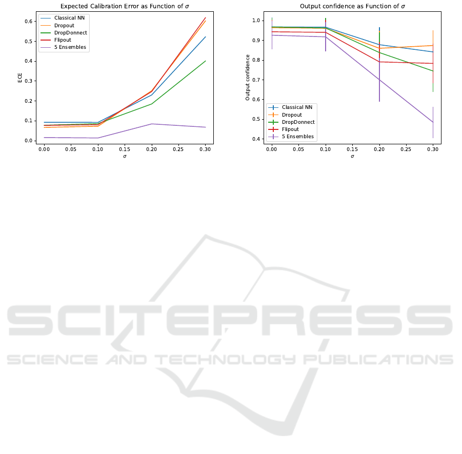
(a) Expected Calibration Error (b) Output conﬁdence as function of input uncertainty σ.

Figure 8: Comparison of Expected Calibration Error and Output conﬁdences for Fashion MNIST as input uncertainty σ is

varied. Note how Ensembles has little variation in calibration error and the largest decrease in conﬁdence with increasing σ.

tary of the normalized uncertainty obtained from

Equation (7).

Finally, due to the ease of visualization provided by

the 2D nature of Two Moons, we plot the dataset and

the uncertainty, calculated in terms of entropy, for a

lattice of points around the dataset.

3 EXPERIMENTAL RESULTS

We perform experiments on two datasets. The pur-

pose of these experiments is to evaluate if a Bayesian

neural network and other models with uncertainty es-

timation, can learn to model input uncertainty from

two inputs (mean and standard deviation). We test

this with a simple setup, we train models with ﬁxed

levels of input uncertainty, and then test with increas-

ing levels of input uncertainty.

Our expectation is, if a model properly learns

the relationship between input and output uncertainty,

then increasing input uncertainty should lead to in-

creases in output uncertainty. We measure output un-

certainty via entropy and maximum softmax conﬁ-

dence, and quality of uncertainty via the expected cal-

ibration error.

3.1 Two Moons Toy Example

We ﬁrst evaluate on a toy example, the Two Moons

dataset, available in scikit-learn, as it allows for easy

control of input uncertainty and to visualize its ef-

fects. We perform two experiments, ﬁrst we train a

model with a single σ value during training, and then

train a model with multiple σ values.

We ﬁrst examine the case for a single training

uncertainty, we use σ = 0.2. We plot and compare

the output entropy distribution over the input domain,

keeping the mean ﬁxed but varying the input uncer-

tainty σ from σ = 0.0 to σ = 2.0. These results are

presented in Figure 2 and detailed plots for two met-

rics in Figure 6.

These results show that only Ensembles and

Flipout signiﬁcantly decrease their output conﬁdence

as the input uncertainty σ increases, while a classical

NN without uncertainty estimation becomes highly

miscalibrated, and other methods only produce mi-

nor decreases in output conﬁdence. No variations in

ECE and output conﬁdence while σ increases indi-

cates that the model might be ignoring the input un-

certainty, which is exactly the behavior we wanted to

test.

We secondly examine the case for mul-

tiple training input uncertainties, using

σ ∈ [0.0, 0.2, 0.4, 0.6, 0.8], and testing with

σ ∈ [0.0, 0.25, 0.5, 0.75, 1.0, 1.25, 1.50, 1.75, 2.0]

progressively. These results are presented in

Figure 7.

These results indicate that Flipout is always mis-

calibrated relative to other methods, and that all un-

certainty estimation methods minus Flipout seem to

be insensitive to input uncertainty, always producing

high output uncertainty. At the end of the spectrum,

training with ﬁve different σ values (Figure 7e), most

methods have learned to ignore the input uncertainty

as output conﬁdence barely varies.

3.2 Fashion-MNIST Image

Classiﬁcation

We then proceed to evaluate our hypothesis on

Fashion-MNIST. We train the models on a ﬁxed stan-

dard deviation value σ = 0.1 and report the corre-

Can Bayesian Neural Networks Explicitly Model Input Uncertainty?

195

Training Data Points

Predictive Mean Predictive Standard Deviation

Dropout

Training σ = 0.20 Testing σ = 0.01 Testing σ = 0.30 Testing σ = 0.50

−10

Testing σ = 0.70

DropConnect

−10

5 Ensembles

−10

0 5 10

Flipout

0 5 10 0 5 10 0 5 10 0 5 10

−10

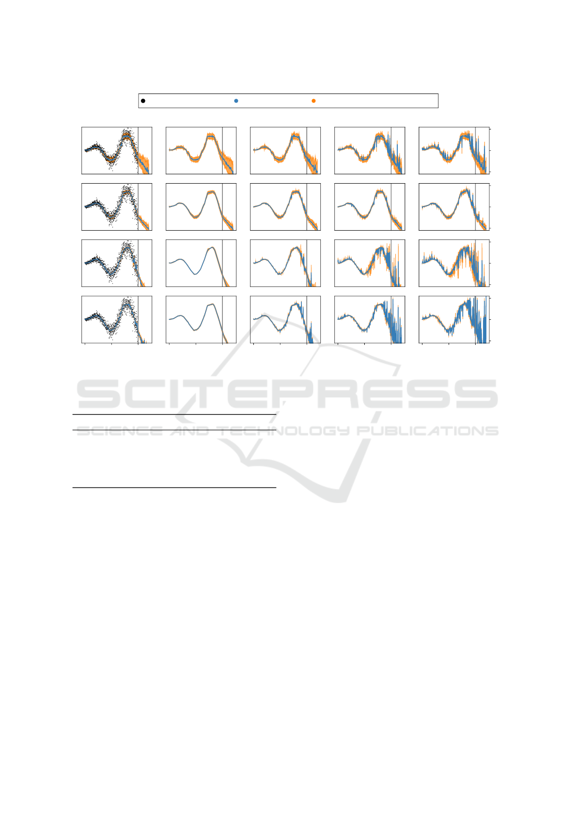
Figure 9: Comparison on a toy regression setting with training σ = 0.2 and variable testing standard deviation. Consistent

with classiﬁcation results, Ensembles and Dropout have the highest sensitivity to input uncertainty σ.

Table 2: Train– and test–set accuracy attained by our NNs

trained on Fashion-MNIST.

Model Train accuracy Test accuracy

Deterministic NN 98.6% 88.6%

MC-Dropout 98.7% 88.7%

MC-DropConnect 98.7% 87.7%

Ensemble 98.5% 88.3%

Flipout 95.5% 85.9%

sponding test-set accuracy in Table 2. ECE and out-

put conﬁdence (computed on the test-set) as function

of input uncertainty are presented in Figure 8. In this

case, we restrict the range of standard deviation for

the testing to σ =0.0, 0.1, 0.2 and 0.3 While we train

on a single input σ, Ensembles and Flipout decrease

their output conﬁdence while input uncertainty σ in-

creases, as expected, while other methods do not. The

results are similar to what we observed on the Two

Moons dataset, indicating that our results and experi-

ments generalize to a more complex image classiﬁca-

tion setting.

3.3 Toy Regression Example

Finally we evaluate results on the toy regression ex-

ample, these results are shown in Figure 9 in terms of

predictions with epistemic uncertainty, and Figure 10

by comparing input and output uncertainties.

Dropout and DropConnect are insensitive to

changes in input uncertainty, mostly by producing

large uncertainties that do not vary with the input un-

certainty, while Ensembles and Flipout do have vary-

ing output uncertainty with the input uncertainty, in

a monotonic way, Flipout has increasing uncertainty

mostly as variations in the predictive mean, while En-

sembles has variation mostly on the standard devia-

tion, so we consider the Ensemble results to be more

representative of our expectations on how output un-

certainty should behave as functions of input uncer-

tainty.

Results on this regression example are consistent

with our previous classiﬁcation results, indicating that

the results are general enough across tasks.

4 CONCLUSIONS

In the present work, we investigated the quality

of modeling aleatoric uncertainty by classical Neu-

ral Networks (NNs) and Bayesian Neural Networks

(BNNs) when the input uncertainty is fed directly to

the models in addition to the canonical input. We pro-

posed a simple setting in which we artiﬁcially injected

Gaussian noise in two famous benchmark datasets—

VISAPP 2025 - 20th International Conference on Computer Vision Theory and Applications

196

0.01 0.25 0.50 0.75 1.00

Input σ

Output σ

Output σ as function of input σ for Dropout

(a) Dropout

0.01 0.25 0.50 0.75 1.00

Input σ

Output σ

Output σ as function of input σ for DropConnect

(b) Dropconnect

0.01 0.25 0.50 0.75 1.00

Input σ

Output σ

Output σ as function of input σ for 5 Ensembles

0.01 0.25 0.50 0.75 1.00

Input σ

Output σ

Output σ as function of input σ for Flipout

(d) Flipout

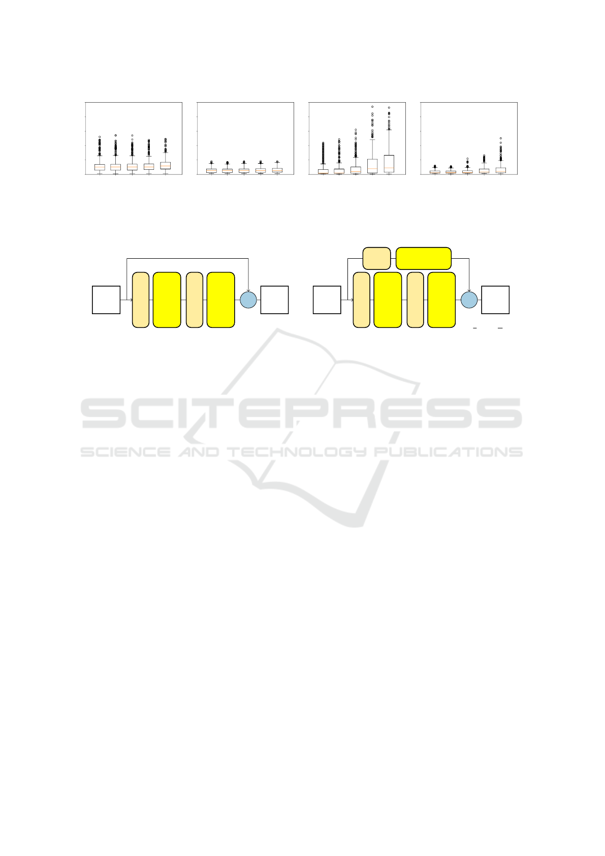
Figure 10: Comparison of output standard deviation as function of input standard deviation for the toy regression setting via

boxplots. Flipout seems barely sensitive to changes in input uncertainty, while Ensembles has the highest reaction to increased

input uncertainty.

(a)

input

shape

h × w × m

BN + ReLU

Conv 3 × 3

n ch., 1 str.

BN + ReLU

Conv 3 × 3

n ch., 1 str.

output

shape

h × w × n

skip connection

(b)

input

shape

h × w × m

BN + ReLU

Conv 3 × 3

n ch., 2 str.

BN + ReLU

Conv 3 × 3

n ch., 1 str.

output

shape

⌈

⌉ × ⌈

⌉ × n

BN +

ReLU

Conv 1 × 1

n ch., 2 str.

skip conn.

Figure 11: Diagrams depicting the two types of residual block used in the Preact-ResNet18 architecture: (a) standard residual

block: a classic residual block with two 3 × 3 convolutions (“Conv”) with a predeﬁned number of output channels n, stride

and padding of 1. The residual blocks are preceded by batch normalization (“BN”) and ReLU activation. The input and output

have the same spatial dimensions h and w. (b) residual block with downsample: it operates a downsampling on the spatial

dimension by modifying the ﬁrst convolution to have a stride of 2 instead of 1. In order to match the spatial dimension after

the two convolutions, the skip connection presents a BN followed by ReLU and a 1 × 1 convolution with stride 2 and padding

1. The output has spatial dimensions which are half the size of the input’s.

Two Moons and Fashion-MNIST—often used in un-

certainty estimation studies. This simulates a natural

environment in which the data are collected by means

of sensors, which always exhibit a certain degree of

noise. For having the models receive the input un-

certainty directly, while this being separated from the

data itself, we crafted a set of NN architectures—

which we dubbed two-input NNs—with two input

channels, one for the mean data and the other for

the standard deviation corresponding to the added

noise. We trained these models on the above men-

tioned datasets, with a ﬁxed level of noise, using ﬁve

approximate BNN techniques: MC-Dropout, MC-

DropConnect, Flipout, Ensembles, and Direct Uncer-

tainty Quantiﬁcation (DUQ).

We tested these models with data with none to

high-levels of noise and proceeded to compute the

output conﬁdence and the Expected Calibration Er-

ror (ECE) as a function of noise. Our hypothesis was

that, generically, these models would exhibit a cer-

tain degree of insensitivity to added noise, where their

conﬁdence would still be high even when data with

high noise—which are effectively out-of-distribution

in the settings—are presented to them. The results are

pointing in this direction: both on Two Moons and

on Fashion-MNIST, the output conﬁdence for most

of the methods remains high, while the Ensembles

show a pronounced drop in conﬁdence as the input

uncertainty increases. On the other hand, the results

elicited by ECE are not conclusive, depicting a nois-

ier scenario for what concerns the (mis)calibration of

the models.

On Two Moons, where we conducted more exten-

sive analyses, we noticed that, after injecting higher

levels of noise in the training process, the models

would essentially start ignoring the signal coming

from the input uncertainty and always produce very

conﬁdent predictions and being less miscalibrated.

Despite this seemingly being an optimal behavior, in

which robustness to noise is enforced, can cause the

NNs to fail at recognizing anomalous data, which is

one of the reasons for adopting BNNs: by providing

more reliable conﬁdence estimates, conﬁdence can be

thresholded to ﬁlter out outliers and avoid classifying

them.

Thus, our analyses suggest that both deterministic

NNs and BNNs fail, in a certain degree, to model data

uncertainty when this one is provided explicitly as

input, with ensembles—which are already known in

the literature to being particularly powerful then other

methods at producing good uncertainty estimates—

and, to a lower extent, Flipout, showing the biggest

Can Bayesian Neural Networks Explicitly Model Input Uncertainty?

197

drop in conﬁdence when presented with very noisy

inputs.

Our work, despite being the ﬁrst analysis on the

uncertainty of the NNs when directly modeling in-

put uncertainty, is still quite small scale and mostly

observational, and could potentially beneﬁt for more

extensive analyses. For instance, larger-scale datasets

might be used—although BNNs are notoriously dif-

ﬁcult and slow to train on bigger datasets. Also, we

could extend the selection of BNN-training schemes

to other methods, like the more recent SWAG (Mad-

dox et al., 2019), or Hamiltonian Monte–Carlo (Neal

et al., 2011), which is still considered the golden stan-

dard for Bayesian modeling, albeit very unfeasible to

apply in the large-scale datasets used in modern Deep

Learning. Finally, our study could beneﬁt from the

addition on the analysis of uncertainty disentangle-

ment by the BNNs, to understand to what extent the

models are able to integrate aleatoric uncertainty into

the input uncertainty.

REFERENCES

Blundell, C., Cornebise, J., Kavukcuoglu, K., and Wier-

stra, D. (2015). Weight uncertainty in neural network.

In Bach, F. and Blei, D., editors, Proceedings of the

32nd International Conference on Machine Learning,

volume 37 of Proceedings of Machine Learning Re-

search, pages 1613–1622, Lille, France. PMLR.

Drucker, H. and Le Cun, Y. (1992). Improving gener-

alization performance using double backpropagation.

IEEE transactions on neural networks, 3(6):991–997.

Gal, Y. and Ghahramani, Z. (2016). Dropout as a bayesian

approximation: Representing model uncertainty in

deep learning. In international conference on machine

learning, pages 1050–1059. PMLR.

Guo, C., Pleiss, G., Sun, Y., and Weinberger, K. Q. (2017).

On calibration of modern neural networks. In Interna-

tional conference on machine learning, pages 1321–

1330. PMLR.

Harris, E., Marcu, A., Painter, M., Niranjan, M., Pr

ugel-

Bennett, A., and Hare, J. (2020). Fmix: Enhanc-

ing mixed sample data augmentation. arXiv preprint

arXiv:2002.12047.

He, K., Zhang, X., Ren, S., and Sun, J. (2016). Identity

mappings in deep residual networks. In Computer

Vision–ECCV 2016: 14th European Conference, Am-

sterdam, The Netherlands, October 11–14, 2016, Pro-

ceedings, Part IV 14, pages 630–645. Springer.

Hinton, G. E., Srivastava, N., Krizhevsky, A., Sutskever, I.,

and Salakhutdinov, R. R. (2012). Improving neural

networks by preventing co-adaptation of feature de-

tectors. arXiv preprint arXiv:1207.0580.

ullermeier, E. (2014). Learning from imprecise and fuzzy

observations: Data disambiguation through general-

ized loss minimization. International Journal of Ap-

proximate Reasoning, 55(7):1519–1534.

ullermeier, E. and Waegeman, W. (2021). Aleatoric and

epistemic uncertainty in machine learning: An intro-

duction to concepts and methods. Machine learning,

110(3):457–506.

Kingma, D. P. and Ba, J. (2014). Adam: A

method for stochastic optimization. arXiv preprint

arXiv:1412.6980.

Kramer, O. and Kramer, O. (2016). Scikit-learn. Machine

learning for evolution strategies, pages 45–53.

Lakshminarayanan, B., Pritzel, A., and Blundell, C. (2017).

Simple and scalable predictive uncertainty estimation

using deep ensembles. Advances in neural informa-

tion processing systems, 30.

LeCun, Y., Bottou, L., Bengio, Y., and Haffner, P. (1998).

Gradient-based learning applied to document recogni-

tion. Proceedings of the IEEE, 86(11):2278–2324.

MacKay, D. J. C. (1992). The evidence framework ap-

plied to classiﬁcation networks. Neural Computation,

4(5):720–736.

Maddox, W. J., Izmailov, P., Garipov, T., Vetrov, D. P., and

Wilson, A. G. (2019). A simple baseline for bayesian

uncertainty in deep learning. Advances in neural in-

formation processing systems, 32.

Naeini, M. P., Cooper, G., and Hauskrecht, M. (2015).

Obtaining well calibrated probabilities using bayesian

binning. In Proceedings of the AAAI conference on

artiﬁcial intelligence, volume 29.

Neal, R. M. et al. (2011). Mcmc using hamiltonian dynam-

ics. Handbook of markov chain monte carlo, 2(11):2.

Nguyen, A., Yosinski, J., and Clune, J. (2015). Deep neural

networks are easily fooled: High conﬁdence predic-

tions for unrecognizable images. In Proceedings of

the IEEE conference on computer vision and pattern

recognition, pages 427–436.

Nix, D. A. and Weigend, A. S. (1994). Estimating the mean

and variance of the target probability distribution. In

Proceedings of 1994 ieee international conference on

neural networks (ICNN’94), volume 1, pages 55–60.

IEEE.

Ovadia, Y., Fertig, E., Ren, J., Nado, Z., Sculley, D.,

Nowozin, S., Dillon, J., Lakshminarayanan, B., and

Snoek, J. (2019). Can you trust your model's uncer-

tainty? evaluating predictive uncertainty under dataset

shift. In Wallach, H., Larochelle, H., Beygelzimer,

A., d'Alch

e-Buc, F., Fox, E., and Garnett, R., editors,

Advances in Neural Information Processing Systems,

volume 32. Curran Associates, Inc.

Papadopoulos, G., Edwards, P. J., and Murray, A. F. (2001).

Conﬁdence estimation methods for neural networks:

A practical comparison. IEEE transactions on neural

networks, 12(6):1278–1287.

Roberts, H. V. (1965). Probabilistic prediction. Journal of

the American Statistical Association, 60(309):50–62.

Rodrigues, N. V., Abramo, L. R., and Hirata, N. S. (2023).

The information of attribute uncertainties: what con-

volutional neural networks can learn about errors in

input data. Machine Learning: Science and Technol-

ogy, 4(4):045019.

Tzelepis, C., Mezaris, V., and Patras, I. (2017). Linear

maximum margin classiﬁer for learning from uncer-

VISAPP 2025 - 20th International Conference on Computer Vision Theory and Applications

198

tain data. IEEE transactions on pattern analysis and

machine intelligence, 40(12):2948–2962.

Valdenegro-Toro, M. (2021a). I ﬁnd your lack of uncer-

tainty in computer vision disturbing. In Proceedings

of the IEEE/CVF Conference on Computer Vision and

Pattern Recognition, pages 1263–1272.

Valdenegro-Toro, M. (2021b). Keras uncertainty. https://

github.com/mvaldenegro/keras-uncertainty.

GitHub repository.

Valdenegro-Toro, M. and Mori, D. S. (2022). A deeper look

into aleatoric and epistemic uncertainty disentangle-

ment. In 2022 IEEE/CVF Conference on Computer

Vision and Pattern Recognition Workshops (CVPRW),

pages 1508–1516. IEEE.

van Amersfoort, J., Smith, L., Teh, Y. W., and Gal, Y.

(2020). Uncertainty estimation using a single deep

deterministic neural network. In International confer-

ence on machine learning, pages 9690–9700. PMLR.

Wan, L., Zeiler, M., Zhang, S., Le Cun, Y., and Fergus, R.

(2013). Regularization of neural networks using drop-

connect. In Dasgupta, S. and McAllester, D., editors,

Proceedings of the 30th International Conference on

Machine Learning, volume 28 of Proceedings of Ma-

chine Learning Research, pages 1058–1066, Atlanta,

Georgia, USA. PMLR.

Wen, Y., Vicol, P., Ba, J., Tran, D., and Grosse,

R. (2018). Flipout: Efﬁcient pseudo-independent

weight perturbations on mini-batches. arXiv preprint

arXiv:1803.04386.

Wright, W. (1998). Neural network regression with input

uncertainty. In Neural Networks for Signal Processing

VIII. Proceedings of the 1998 IEEE Signal Processing

Society Workshop (Cat. No. 98TH8378), pages 284–

293. IEEE.

Wright, W. (1999). Bayesian approach to neural-network

modeling with input uncertainty. IEEE Transactions

on Neural Networks, 10(6):1261–1270.

Xiao, H., Rasul, K., and Vollgraf, R. (2017). Fashion-

mnist: a novel image dataset for benchmark-

ing machine learning algorithms. arXiv preprint

arXiv:1708.07747.

Can Bayesian Neural Networks Explicitly Model Input Uncertainty?

199