Exploring Local Graphs via Random Encoding
for Texture Representation Learning
Ricardo T. Fares
a
, Luan B. Guerra
b
and Lucas C. Ribas
c
S
˜
ao Paulo State University (UNESP), Institute of Biosciences, Humanities and Exact Sciences, S
˜
ao Jos
´
e do Rio Preto, Brazil
Keywords:
Texture Representation, Randomized Neural Networks, Graph-Based Modeling.
Abstract:
Despite many graph-based approaches being proposed to model textural patterns, they not only rely on a large
number of parameters, culminating in a large search space, but also model a single, large graph for the entire
image, which often overlooks fine-grained details. This paper proposes a new texture representation that uti-
lizes a parameter-free micro-graph modeling, thereby addressing the aforementioned limitations. Specifically,
for each image, we build multiple micro-graphs to model the textural patterns, and use a Randomized Neu-
ral Network (RNN) to randomly encode their topological information. Following this, the network’s learned
weights are summarized through distinct statistical measures, such as mean and standard deviation, generating
summarized feature vectors, which are combined to form our final texture representation. The effectiveness
and robustness of our proposed approach for texture recognition was evaluated on four datasets: Outex, USP-
tex, Brodatz, and MBT, outperforming many literature methods. To assess the practical application of our
method, we applied it to the challenging task of Brazilian plant species recognition, which requires microtex-
ture characterization. The results demonstrate that our new approach is highly discriminative, indicating an
important contribution to the texture analysis field.
1 INTRODUCTION
Texture is an essential attribute present in numerous
natural objects and scenes. Despite the absence of
a formally established definition of texture, it can be
understood as the spatial layout of intensities within
a local neighborhood of a pixel. In living beings, the
visual cortex is responsible for processing and encod-
ing textural information into complex representations,
enabling the recognition of various surfaces and ma-
terials (Jagadeesh and Gardner, 2022). To bring sim-
ilar recognition capabilities to computers, researchers
have developed texture descriptors that numerically
express these features in one-dimensional vectors, en-
abling its application in numerous tasks, such as tissue
classification (Kruper et al., 2024), environment mon-
itoring (Borzooei et al., 2024) and remote sensing (Xu
et al., 2024).
Initially, automated texture encoding approaches
relied on classical or hand-engineered methods, in
which the textural encoding processes were manu-
a
https://orcid.org/0000-0001-8296-8872
b
https://orcid.org/0009-0004-3278-9306
c
https://orcid.org/0000-0003-2490-180X
ally designed by specialists. Examples of such ap-
proaches include: the Gray-Level Co-occurrence Ma-
trix (GLCM) (Haralick, 1979), which extracts k-th or-
der statistical information to describe the distribution
of local patterns of the pixel neighborhoods, and Lo-
cal Binary Patterns (LBP) (Ojala et al., 2002b), which
encodes pixel neighborhoods into unique values that
are then aggregated into a histogram. However, due to
the increasing complexity of images generated by di-
verse real-world applications, these approaches often
struggle to handle this complexity and fail to achieve
satisfactory results.
To address this, various learning-based ap-
proaches have been developed that rely on large ar-
tificial neural networks, such as Convolutional Neural
Networks (CNNs) and Vision Transformers (ViTs),
which automatically learn to extract useful visual fea-
tures by minimizing a loss function. Examples of
such architectures are: VGG19 (Simonyan and Zis-
serman, 2014), InceptionV3 (Szegedy et al., 2016),
ResNet50 (He et al., 2016), and InceptionResNetV2
(Szegedy et al., 2017). Although these models have
achieved superior results across many tasks, they are
often constrained by limited training data, a challenge
commonly encountered in certain applications, such
200
Fares, R. T., Guerra, L. B. and Ribas, L. C.
Exploring Local Graphs via Random Encoding for Texture Representation Learning.
DOI: 10.5220/0013315500003912
Paper published under CC license (CC BY-NC-ND 4.0)
In Proceedings of the 20th International Joint Conference on Computer Vision, Imaging and Computer Graphics Theory and Applications (VISIGRAPP 2025) - Volume 3: VISAPP, pages
200-209
ISBN: 978-989-758-728-3; ISSN: 2184-4321
Proceedings Copyright © 2025 by SCITEPRESS – Science and Technology Publications, Lda.

as medicine, which can lead to optimization issues.
In this sense, to harness the advantages of hand-
engineered approaches, known for their invariance to
the need for large datasets, alongside the automatic
feature extraction of learning-based approaches, re-
cent texture representation techniques have employed
randomized neural networks (RNNs) (S
´
a Junior and
Backes, 2016; Ribas et al., 2024a; Fares and Ribas,
2024) for pattern recognition tasks. These networks
are both simple and fast-learning, as their training
phase is conducted via a closed-form solution, elimi-
nating the need for backpropagation. In these investi-
gations, a randomized neural network is trained for
each image, with the learned weights used to con-
struct the texture representation. However, the ef-
fectiveness of this texture descriptor largely depends
on the construction of the input feature matrix (local
patches), which provides the information to be ran-
domly encoded.
In particular, several RNN-based approaches,
such as in (Ribas et al., 2020; Ribas et al., 2024a;
Ribas et al., 2024b) use graphs, a well-known math-
ematical tool, to model relationships among textural
patterns in the image. However, the graph modeling
in these approaches requires between 1 and 4 hyper-
parameters to be calibrated, resulting in a large search
space of parameter combinations. Additionally, these
approaches model the entire image as a single large
graph, which may overlook finer texture details and
introduce scalability issues due to the graph size rela-
tive to image resolution.
In this paper, we introduce a novel texture repre-
sentation approach that (1) employs hyperparameter-
free graph modeling by utilizing multiple micro-
graphs to capture local textural information in the im-
age; and (2) uses randomized neural networks to ran-
domly encode these micro-graphs in the network’s
learned weights. Specifically, to build the represen-
tation, we center a 3 × 3 local patch on each pixel
of the image, construct a micro-graph to model this
patch, and extract topological measures. From this,
the pixel intensities of the patches form the input fea-
ture matrix, and the topological measures of the mod-
eled graph the output one. These matrices are then
used to feed a randomized neural network (RNN),
where the network’s learned weights are summarized
using statistical measures. Each statistical measure
generates a distinct statistical vector, which is then
combined to compose our final texture representation.
In summary, the main contributions of our work are:
(i) A parameter-free graph modeling approach. (ii) A
compact and low-cost representation via RNNs. (iii)
Invariance to the dataset size. (iv) Promising results in
the challenging task of Brazilian plant species recog-
nition.
Finally, the paper is organized as follows. In Sec-
tion 2, we describe the proposed methodology. In
Section 3, we present the experimental setup, results,
discussion, and comparisons. Lastly, in Section 4 we
conclude the paper.
2 PROPOSED METHOD
2.1 Randomized Neural Networks
Randomized neural network is a simple neural net-
work model composed by a single fully-connected
hidden layer whose weights are randomly gener-
ated by some probability distribution (Huang et al.,
2006; Pao and Takefuji, 1992; Pao et al., 1994;
Schmidt et al., 1992). The objective is to randomly
project the input into a higher dimensional space,
thereby enhancing the probability of the data becom-
ing more linearly separable, as stated in Cover’s the-
orem (Cover, 1965). Following this, the weights of
the output layer are learned through a closed-form so-
lution, i.e. gradient-free, to minimize a least-squares
error optimization problem.
Mathematically, let X = [⃗x
1
,⃗x
2
,... ,⃗x
N
] ∈ R
p×N
,
where ⃗x
i
∈ R
p
be the input feature matrix com-
posed of N input feature vectors, and let Y =
[⃗y
1
,⃗y
2
,. .. ,⃗y
N
] ∈ R
r×N
, where ⃗y
i
∈ R
r
be the output
feature matrix consisting of N output feature vec-
tors. Further, let W ∈ R
Q×(p+1)
be the randomly
generated weight matrix, with Q being the number
of hidden neurons, and with the first column being
the bias’ weights. Lastly, let 1
1
1
N
be a row matrix
with N columns with all entries set as 1, and define
X
′
= [−1
1
1
T
N
X
T
]
T
as the input feature matrix with the
bias appended.
From this, we can compute the forward step by
U = φ(WX), where φ is the sigmoid function, and
U = [⃗u
1
,⃗u
2
,. .. ,⃗u
N
] ∈ R
Q×N
, where⃗u ∈ R
Q
is the ma-
trix consisting of the N randomly projected input fea-
ture vectors in the Q-dimensional space. Further, we
define Z = [−1
1
1
T
N
U
T
]
T
as the projected feature ma-
trix with the bias added.
From this, we can calculate the output layer
weights by the following closed-solution formula:
M = YZ
T
(ZZ
T
)
−1
, (1)
where Z
T
(ZZ
T
)
−1
is the Moore-Penrose pseudo-
inverse (Moore, 1920; Penrose, 1955). Neverthe-
less, there may be cases where ZZ
T
is ill-conditioned,
producing unstable inverses. To tackle this issue,
Tikhonov regularization (Tikhonov, 1963; Calvetti
et al., 2000) is applied, by adjusting the formula to:
Exploring Local Graphs via Random Encoding for Texture Representation Learning
201

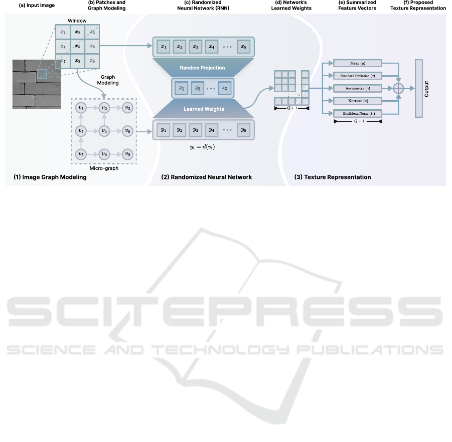
Figure 1: Illustration of the process to obtain the texture representation from the (a) input image to (f) the proposed texture
representation. The steps include (b) micro-graph modeling of the local patches, which are then applied to a (c) RNN to
produce the (d) network’s learned weights. These weights are (e) summarized and subsequently combined to form the (f)
proposed texture representation.
M = YZ
T
(ZZ
T
+ λI)
−1
, where λ > 0 is the regular-
ization parameter, and I ∈ R
(Q+1)×(Q+1)
is the identity
matrix. Finally, we set λ = 10
3
as suggested in other
investigations (Fares et al., 2024).
2.2 Learning Texture Representation
The key idea underlying our approach is that, un-
like other graph-based methods that construct a single
large graph to model the entire image texture, we in-
stead create multiple micro-graphs centered on each
pixel of the image, enabling us to capture finer tex-
ture details. We then extract topological measures
from these micro-graphs and use them in a random-
ized neural network. Finally, the network’s learned
weights are summarized to construct the texture rep-
resentation.
To construct the representation of an image I ∈
R
H×W
, we start by creating the input feature matrix
X and the output feature matrix Y. For each pixel
in I, we center a 3 × 3 window to capture their lo-
cal spatial relationships, flatten and concatenate them
to form the matrix X ∈ R
9×HW
. Furthermore, each
window is modeled as a micro-graph composed by 9
vertices (one per pixel) with a directed edge e
i j
going
from vertex v
i
to v
j
when P(v
i
) > P(v
j
), where P(v)
denotes the intensity level of the pixel corresponding
to the vertex v (note that micro-graph in Figure 1(b)
illustrates only some edges, to not clutter the image).
This micro-graph is then converted into a vector con-
taining the out-degrees of each vertex, where the out-
degree d(v) is the number of outgoing edges from v.
This process produces a vector per local window, and
by concatenating these vectors across all windows, we
form the matrix Y ∈ R
9×HW
. This process is depicted
in Figure 1(a) and 1(b).
With X and Y constructed, we applied it to a ran-
domized neural network and obtained the network’s
learned weights, M, using the regularized form of
Equation 1. These learned weights capture essential
information about the textural content encoded by the
pixel intensities and topological measures (e.g., out-
degrees), as the network is trained to predict one us-
ing the other. Thus, from this matrix, we defined our
following summarized feature vector:
⃗
Θ
f
(Q) = [ f (⃗m
1
), f (⃗m
2
),. .. , f (⃗m
Q+1
)], (2)
where f is a statistical measure function (µ for aver-
age, σ for standard deviation, γ for skewness, κ for
kurtosis, and ℓ for ℓ
2
norm squared), ⃗m
k
denotes the
k-th column of the matrix M, and f (⃗m
k
) indicates the
measure function applied over the values at the k-th
column.
From this, we create the partial feature vector by
incorporating different statistical measure functions.
In particular, we applied four statistical measures: av-
erage, standard deviation, skewness and kurtosis (see
Table 1), and one ℓ
2
norm function. This approach
positively contributes to the representation, as differ-
ent statistical perspectives are taken into account, as
investigated in (Fares et al., 2024). Thus, we define it
as:
⃗
Ω(Q) = [
⃗
Θ
µ
(Q),
⃗
Θ
σ
(Q),
⃗
Θ
γ
(Q),
⃗
Θ
κ
(Q),
⃗
Θ
ℓ
(Q)]. (3)
The representation
⃗
Ω(Q) is uniquely determined
by Q, the dimension of the projection space.
VISAPP 2025 - 20th International Conference on Computer Vision Theory and Applications
202

Since different projection space dimensions randomly
project the features in distinct ways, unique infor-
mation can be captured during the prediction phase.
Hence, we define our proposed texture representation
as:
⃗
Φ(Q) = [
⃗
Ω(Q
1
),
⃗
Ω(Q
2
),. .. ,
⃗
Ω(Q
L
)], (4)
where Q = (Q
1
,Q
2
,. .. ,Q
L
).
To conclude, feature extraction methods must en-
sure reproducibility by generating the same feature
vector for the same input image in all executions. For
this purpose, this investigation employed the same
random weight matrix for projecting each input fea-
ture matrix across all images and runs. Specifically,
as extensively employed in previously RNN-based in-
vestigations (S
´
a Junior and Backes, 2016; Ribas et al.,
2020; Ribas et al., 2024b; Fares et al., 2024), the ran-
dom matrix was generated using a Linear Congru-
ent Generator (LCG), defined by the recurrent for-
mula V (n + 1) = (aV (n) + b) mod c, where V is the
vector of length L = Q × (p + 1), with parameters
V (0) = L +1, a = L +2, b = L +3, and c = L
2
. Lastly,
the vector V is standardized, and W is obtained by re-
shaping V into (Q, p + 1) dimensions.
Table 1: Statistical measures formulas utilized to summa-
rize the network’s learned weights.
Average Standard Deviation
µ(⃗v) =
1
N
N
∑
k=1
v
k
σ(⃗v) =
s
1
N − 1
N
∑
k=1
(v
k
− µ(⃗v))
2
Skewness
γ(⃗v) =
1
N
N
∑
k=1
(v
k
−µ(⃗v))
3

s
1
N − 1
N
∑
k=1
(v
k
−µ(⃗v))
2

3
Kurtosis
κ(⃗v) =
1
N
N
∑
k=1
(v
k
−µ(⃗v))
4

s
1
N − 1
N
∑
k=1
(v
k
−µ(⃗v))
2

4
3 EXPERIMENTS AND RESULTS
3.1 Experimental Setup
To assess the effectiveness of our proposed approach,
we conducted experiments on four different texture
datasets, organized as follows:
• Outex (Ojala et al., 2002a): This dataset com-
prises 1360 samples distributed across 68 classes,
each containing 20 images, each of size 128×128
pixels.
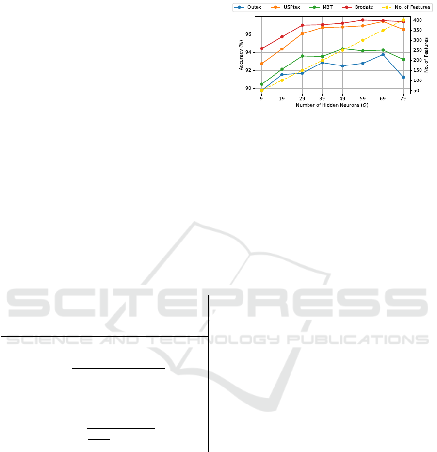
Figure 2: Classification accuracy rate (%) behavior of each
evaluated dataset for various number of hidden neurons (Q)
for the texture descriptor
⃗
Ω(Q).
• USPtex (Backes et al., 2012): The USPtex dataset
includes 2292 images divided into 191 natural
texture classes, with each class consisting of 12
images sized 128 × 128 pixels.
• Brodatz (Brodatz, 1966): This dataset contains
1776 texture samples grouped into 111 classes as
structured in (Backes et al., 2013a), with each
class containing 16 images of size 128 × 128 pix-
els.
• MBT (Abdelmounaime and Dong-Chen, 2013):
Comprising 2464 samples, this dataset captures
intra-band and inter-band spatial variations across
154 classes, each class featuring 16 images with
dimensions of 160 × 160 pixels.
In this investigation, we evaluate the efficacy of
the proposed technique against other methods in the
literature by comparing its performance in terms of
accuracy. The accuracy was obtained using Linear
Discriminant Analysis (LDA) followed by a leave-
one-out cross-validation strategy. In addition, the im-
ages were converted to grayscale before extracting the
texture descriptors.
3.2 Parameter Analysis
Given that our proposed approach relies on a single
parameter, the number of hidden neurons (Q, repre-
senting the dimension of the random projection), we
evaluated its impact on the quality of the texture de-
scriptor by measuring accuracy across four datasets
for each value in Q = 9, 19, . . . , 79. As shown in
Fig. 2, accuracy exhibits an upward trend across all
datasets up to Q = 69. However, at Q = 79, this trend
stops, with a decrease in accuracy observed across
all datasets, indicating that higher-dimensional pro-
jections may not yield additional improvements.
In this sense, to leverage the robustness of lower-
dimensional projections, we designed the texture de-
scriptor
⃗
Φ(Q
1
,Q
2
,. .. ,Q
L
) that combines the learned
Exploring Local Graphs via Random Encoding for Texture Representation Learning
203

Table 2: Classification accuracy rates (%) of each evaluated
dataset and the average accuracy of the proposed texture
descriptor
⃗
Φ(Q
1
,Q
2
). Bold rows denote the configurations
that achieved the two highest average accuracies.
(Q
1
,Q
2
) No. of Features Outex USPtex MBT Brodatz Avg.
(09, 19) 150 91.54 95.90 93.38 96.45 94.32
(09, 29) 200 92.57 96.64 94.28 97.30 95.20
(09, 39) 250 93.09 97.21 95.05 97.18 95.63
(09, 49) 300 92.79 97.08 94.81 97.47 95.54
(09, 59) 350 93.16 97.08 94.28 97.35 95.47
(09, 69) 400 93.60 97.73 94.81 97.75 95.97
(09, 79) 450 91.69 96.86 93.79 97.52 94.97
(19, 29) 250 92.65 96.99 94.40 97.24 95.32
(19, 39) 300 93.46 97.03 94.76 96.96 95.55
(19, 49) 350 92.72 97.16 95.05 97.30 95.56
(19, 59) 400 93.16 97.51 94.64 97.86 95.79
(19, 69) 450 93.75 97.86 95.09 97.24 95.99
(19, 79) 500 92.65 97.47 94.07 97.35 95.39
(29, 39) 350 93.31 97.34 95.01 97.58 95.81
(29, 49) 400 92.65 97.47 94.72 97.86 95.68
(29, 59) 450 92.79 97.60 94.44 97.97 95.70
(29, 69) 500 93.75 97.82 94.68 97.58 95.96
(29, 79) 550 92.35 97.51 94.20 97.97 95.51
(39, 49) 450 94.49 97.77 94.60 97.75 96.15
(39, 59) 500 93.53 97.56 94.93 97.97 96.00
(39, 69) 550 93.60 97.77 94.72 97.92 96.00
(39, 79) 600 92.65 97.60 94.44 97.64 95.58
(49, 59) 550 93.31 97.56 94.85 97.47 95.80
(49, 69) 600 93.53 97.99 94.93 97.69 96.04
(49, 79) 650 92.72 97.47 95.13 97.64 95.74
(59, 69) 650 92.94 97.86 94.64 98.09 95.88
(59, 79) 700 92.50 97.82 94.60 97.52 95.61
(69, 79) 750 93.01 97.64 94.20 97.97 95.71
feature vectors for each distinct number of hidden
neurons. Therefore, our second experiment evaluated
the performance of the proposed descriptor by mea-
suring the average accuracy across the four datasets
for every possible combination of two hidden neuron
values in {(Q
1
,Q
2
) ∈ Q × Q | Q
1
< Q
2
}, thus allow-
ing us to observe its behavior.
From Table 2, it is noteworthy that even for the
same number of features, the proposed texture repre-
sentation
⃗
Φ(Q
1
,Q
2
), produced by combining two hid-
den neurons, achieved higher accuracies than a sin-
gle neuron representation,
⃗
Ω(Q). For instance, the
combined representation
⃗
Φ(09,39) achieved an av-
erage accuracy of 95.63%, whereas
⃗
Ω(49) achieved
only 95.24%, both using 250 attributes. This in-
dicates that the texture descriptor based on multi-
ple lower-dimensional projections is more robust than
one learned from a single higher-dimensional projec-
tion, thereby opening margins for further improve-
ments.
Thus, these improvements are demonstrated
by other combinations, such as
⃗
Φ(39,49), which
achieved the highest average accuracy of 96.15% with
only 450 attributes, presenting it as a robust and dis-
criminative compact texture descriptor. This result
is particularly beneficial, as reasonably small feature
vectors reduce both computation and inference costs.
Therefore, based on this, we selected the compact
texture representations
⃗
Φ(39,49) and
⃗
Φ(19,69) both
with 450 attributes, which achieved the first and the
fifth average accuracies, respectively, to be compared
against other methods in the literature.
3.3 Comparison and Discussions
To assess the competitiveness of our proposed tex-
ture representation, we compared it with other meth-
ods from the literature. The experimental setup was
the same as the preceding section, using LDA with
leave-one-out cross-validation, except for the CLBP
method, which used a 1-Nearest Neighbor (1-NN)
classifier.
We compared our method with three categories of
descriptors: hand-engineered, RNN-based, and deep
convolutional neural network (DCNN) approaches,
as shown in the first, second, and third labeled row
blocks of Table 3, respectively. For the DCNNs,
we specifically used pre-trained models on ImageNet
(Deng et al., 2009), employing them as feature ex-
tractors by applying Global Average Pooling (GAP)
to the last convolutional layer, as suggested in a pre-
vious study (Ribas et al., 2024b).
Firstly, we compared our proposed approach
against hand-engineered methods. Thus, as shown
in Table 3 our both proposed descriptors,
⃗
Φ(39,49)
and
⃗
Φ(19,69), achieved higher accuracies than hand-
engineered methods across all datasets. For in-
stance,
⃗
Φ(39,49) reached an accuracy of 94.49%
on Outex, while AHP only achieved 88.31%, a no-
table difference of 6.18%. On USPtex,
⃗
Φ(39,49)
achieved 97.77%, while AHP obtained 94.85%, an
improvement of 2.92%. Furthermore, our approach
obtained 97.75% on Brodatz, outperforming CLBP,
which achieved 95.32%, by a difference of 2.43%.
Finally, on MBT,
⃗
Φ(19,69) obtained 95.09%, while
GLDM reached 92.78%, representing an increase of
2.31%. Therefore, these findings highlight the poten-
tial of our approach which uses a graph-based mod-
eling and a simple neural network in relation to the
hand-engineered approaches.
Following this, in the second part of Table 3,
we present a comparison between our approach and
other RNN-based methods. Notably, our proposed
descriptors,
⃗
Φ(39,49) and
⃗
Φ(19,69), outperformed
all RNN-based approaches on the Outex, Brodatz
and MBT datasets, and ranked second on the USP-
tex dataset achieving an accuracy of 97.86% by
⃗
Φ(19,69), whereas the first, REE (Fares et al., 2024),
achieved 98.08%, showing a small margin of 0.22%
of increment. This improvement suggests that pre-
dicting the micro-graphs topological information us-
ing the pixel intensities instead of only using the pixel
intensities directly as other RNN-based approaches
do, allowed the network to learn more meaningful in-
formation, culminating in improved accuracies.
VISAPP 2025 - 20th International Conference on Computer Vision Theory and Applications
204

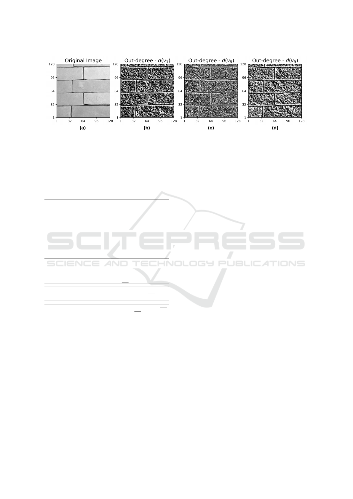
Figure 3: Illustration of enhancement of the underlying image properties by the micro-graph modeling. (a) presents the
original images, whereas (b), (c) and (d) presents the visual representations of the out-degree values used as pixel intensity.
The images (b) and (d) enhances the roughness information, which can hardly be seen in (a), and (c) enhances the granularity
information of (a), therefore, capturing key image patterns.
Table 3: Comparison of classification accuracies of various
texture analysis. A subset of these results was sourced from
(Ribas et al., 2020), and (Ribas et al., 2024a). Empty cell
indicate that the result is unavailable. Bold text indicates
the best result, and underlined text the second-best.
Methods # Features Outex USPTex Brodatz MBT
Hand-engineered Approaches
GLCM (Haralick, 1979) 24 80.73 83.64 90.43 85.88
GLDM (Weszka et al., 1976) 60 86.76 92.06 94.43 92.78
Gabor Filters (Manjunath and Ma, 1996) 48 81.91 89.22 89.86 89.94
Fourier (Weszka et al., 1976) 63 81.91 67.50 75.90 −
Fractal (Backes et al., 2009) 69 80.51 78.27 87.16 −
Fractal Fourier (Florindo and Bruno, 2012) 68 68.38 59.47 71.96 −
LBP (Ojala et al., 2002b) 256 81.10 85.43 93.64 84.74
LBPV (Guo et al., 2010b) 555 75.66 54.97 86.26 73.54
CLBP (Guo et al., 2010a) 648 85.80 91.14 95.32 80.28
AHP (Zhu et al., 2015) 120 88.31 94.85 94.88 85.35
BSIF (Kannala and Rahtu, 2012) 256 77.43 77.66 91.44 79.71
LCP (Guo et al., 2011) 81 86.25 91.14 93.47 84.13
LFD (Maani et al., 2013) 276 82.57 83.55 90.99 80.20
LPQ (Ojansivu and Heikkil
¨
a, 2008) 256 79.41 85.12 92.51 74.64
CNTD (Backes et al., 2013b) 108 86.76 91.71 95.27 83.70
LETRIST (Song et al., 2018) 413 82.80 92.40 − 79.10
RNN-based Approaches
ELM Signature (S
´
a Junior and Backes, 2016) 180 89.71 95.11 95.27 −
CNRNN (Ribas et al., 2020) 240 91.32 96.95 96.06 91.23
SSR
1
(Ribas et al., 2024a) (grayscale) 630 90.80 95.80 − 90.10
SSR
2
(Ribas et al., 2024a) (grayscale) 990 91.60 96.30 − 91.00
LCFNN (Ribas et al., 2024b) 330 92.13 97.21 98.09 −
REE
1
(Fares et al., 2024) 450 93.82 98.08 97.07 93.95
DCNN-based Approaches
VGG19 (Simonyan and Zisserman, 2014) 512 76.62 93.19 96.79 87.42
InceptionV3 (Szegedy et al., 2016) 2048 86.40 96.77 98.54 82.14
ResNet50 (He et al., 2016) 2048 65.66 62.30 81.98 85.51
InceptionResNetV2 (Szegedy et al., 2017) 1536 85.88 96.34 98.99 88.60
Proposed Approach
⃗
Φ(39,49) 450 94.49 97.77 97.75 94.60
⃗
Φ(19,69) 450 93.75 97.86 97.24 95.09
Further, in the third categorization of Table 3,
we compared our technique with some DCNNs, be-
ing them: VGG19, InceptionV3, ResNet50 and In-
ceptionResNetV2. Notably, on the Outex dataset,
our descriptor
⃗
Φ(39,49) demonstrated an improve-
ment, achieving an accuracy of 94.49%, compared
to 86.40% of InceptionV3, representing a significant
difference of 8.09%. This is an outstanding result,
highlighting that while our texture descriptor effec-
tively captures these textures, DCNNs exhibit cer-
tain limitations. On the USPtex dataset, our approach
⃗
Φ(19,69) achieved 97.86%, compared to 96.77% by
InceptionV3, an improvement of 1.09%.
On the Brodatz dataset, the DCNNs architectures
InceptionV3 and InceptionResNetV2 achieved an ac-
curacy of 98.54% and 98.99%, respectively, being
the first and second-best accuracy, while our pro-
posed descriptors,
⃗
Φ(39,49) and
⃗
Φ(19,69), achieved
97.75% and 97.24%, ranking in third and fourth, re-
spectively. Nevertheless, the InceptionV3 and Incep-
tionResNetV2 used 2048 and 1536 attributes, which
might be undesirable due to inference costs. Lastly,
on the MBT dataset, both our approaches,
⃗
Φ(39,49)
and
⃗
Φ(19,69), also presented a considerable im-
provement of 6.00% and 6.49%, by achieving 94.60%
and 95.09%, respectively, in relation to InceptionRes-
NetV2 accuracy of 88.60%. Here, the inefficiency of
the DCNNs may be attributed to the intra-band spatial
variations of the MBT textures. Thus, these results in-
dicate the robustness of our simple and fast-learning
model, compared to the presented DCNNs which are
larger and have higher computational costs.
Finally, in comparison to other graph-based
approaches, such as CNTD, CNRNN, SSR, and
LCFNN, our proposed texture representation sur-
passed all of them across all evaluated datasets. For
instance, while LCFNN (Ribas et al., 2024b) achieved
92.13% on Outex, our approach
⃗
Φ(39,49) reached
94.49%, a significant improvement of 2.36%, and
while CNRNN (Ribas et al., 2020) achieves 91.23%
on MBT, our descriptor
⃗
Φ(19,69) achieved 95.09%,
an improvement of 3.86%. Therefore, these results in-
dicate that leveraging topological measures of micro-
graphs to model texture offers a more robust and dis-
criminative approach than constructing a single graph
for the entire image.
3.4 Qualitative Assessment
To complement the quantitative results presented in
the preceding section, we evaluate the qualitative as-
pects of the proposed approach in this section, demon-
strating its robustness. As micro-graph modeling
is a core element of our approach, designed to en-
Exploring Local Graphs via Random Encoding for Texture Representation Learning
205

hance and extract meaningful patterns from the im-
age, we evaluate its effectiveness in describing the im-
age properties.
To show this, Figure 3(a) plots the original im-
age, and Figure 3(b), 3(c) and 3(d) plot the graphical
representations of the out-degree measure, d(v), rep-
resented as a pixel intensity for the first (v
1
), the fifth
(v
5
) and the ninth (v
9
) vertices of the micro-graph.
In Figure 3(a), the roughness and a smooth gran-
ularity presented in the image can hardly be seen.
Thus, by modeling the image using micro-graphs, and
by analyzing the Figures 3(b), 3(c) and 3(d) that show
the out-degree of vertices resulting from our micro-
graph modeling. It can be seen that the micro-graph
topological information effectively captured and en-
hanced the roughness and granularity, highlighting
these key underlying properties of the image.
Specifically, Figure 3(b) and 3(d) presented the
vertices which enhanced the roughness information,
and 3(c) presented the vertex which enhanced the
granularity content. Thus, these topological informa-
tion enhancing different parts of the image are, there-
fore, predicted from the latent space, forcing the net-
work to learn these patterns, thereby capturing the es-
sential information.
In summary, as demonstrated in the quantitative
results, our approach achieved high accuracy. This
success can largely be attributed to the topological in-
formation provided into the randomized neural net-
work. As shown in this section, the topological mea-
sures capture the essential image details, allowing the
model to learn relevant and insightful texture informa-
tion. This highlights the effectiveness of the micro-
graph modeling in our approach.
3.5 Brazilian Plant Species Recognition
The identification of plant species is essential for
many fields of knowledge, such as medicine and
botany, and is commonly performed using images
from leaves, seeds, and fruits, among others. How-
ever, accurately identifying species based on leaf sur-
faces is a challenging task due to high inter-class sim-
ilarity, high intra-class variability, and environmental
conditions (e.g., sun and rain) that can alter leaf char-
acteristics. Consequently, many studies are exploring
automated identification techniques based on leaf sur-
faces using machine learning tools to improve their
performance.
In this context, we evaluated our proposed
methodology for plant species recognition using leaf
surfaces, showing its effectiveness in an important
practical application. We used the 1200Tex dataset
(Backes et al., 2009), which includes 400 images of
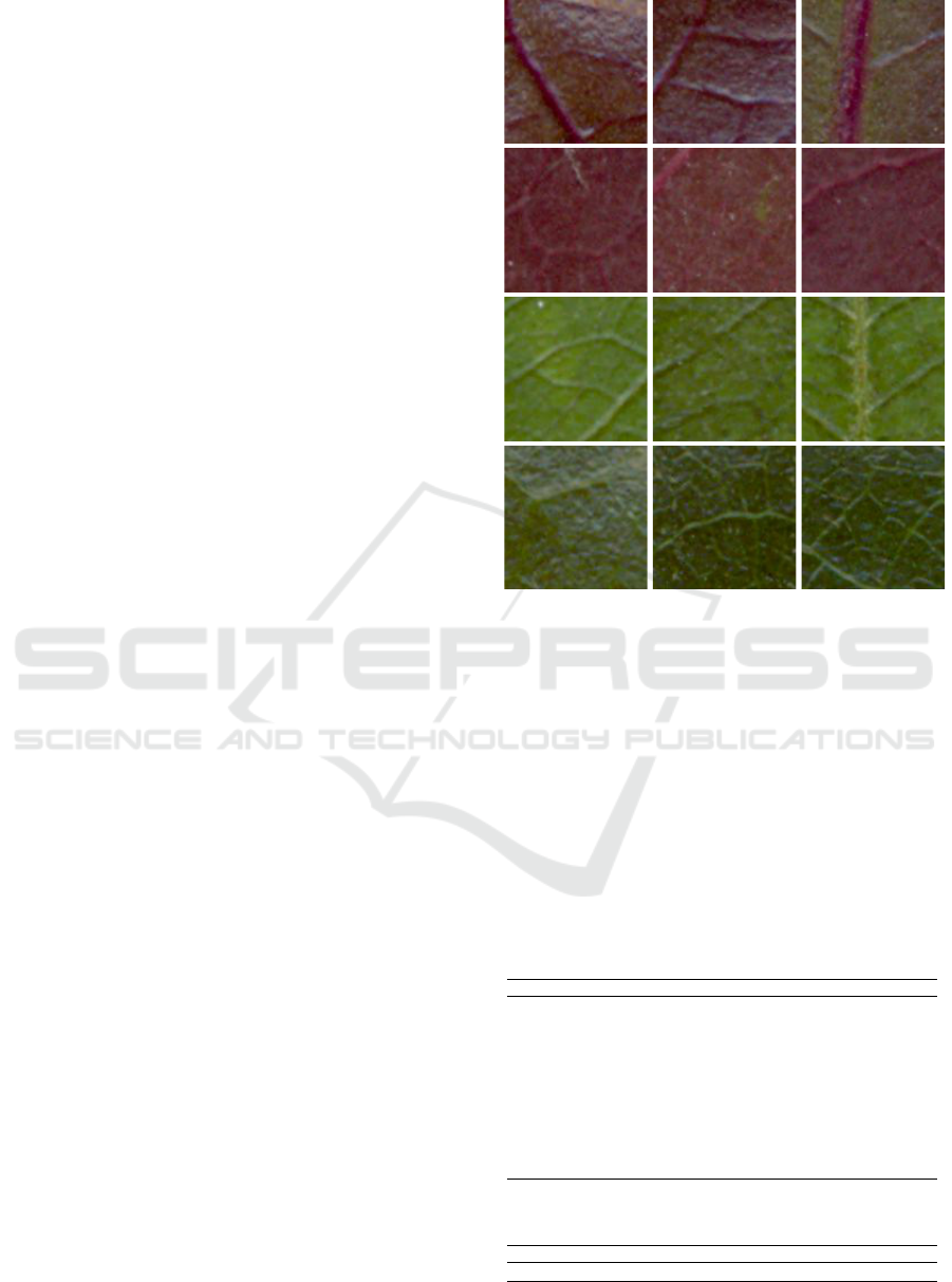
Figure 4: Plant foliar surfaces of the 1200Tex dataset. Each
row presents a different class, and each column shows a dis-
tinct sample of the same class.
leaves divided into 20 classes, each with 20 sam-
ples. For textural analysis, these images were divided
into three non-overlapping windows of 128×128 pix-
els, resulting in 1200 images. Figure 4 provides
sample images from different classes for illustration.
For comparison, we employed the same experimental
setup as the previous section.
Table 4: Classification accuracy rates of distinct literature
methods for texture analysis applied to plant species iden-
tification using foliar surfaces. Results were sourced from
(Ribas et al., 2024a) or taken from their original paper.
Method # Features Accuracy (%)
GLDM (Weszka et al., 1976) 60 79.92
AHP (Ojansivu and Heikkil
¨
a, 2008) 120 79.17
LCP (Guo et al., 2011) 81 76.58
LFD (Maani et al., 2013) 276 74.67
LPQ (Ojansivu and Heikkil
¨
a, 2008) 256 73.00
Fourier (Weszka et al., 1976) 63 65.75
Fractal (Backes et al., 2009) 69 70.75
Gabor (Manjunath and Ma, 1996) 48 77.25
CNTD (Backes et al., 2013b) 108 83.33
RNN-CT (Zielinski et al., 2022) 240 87.08
REE
2
(Fares et al., 2024) 540 88.58
VGG19 (Simonyan and Zisserman, 2014) 512 78.33
ResNet50 (He et al., 2016) 2048 69.33
InceptionV3 (Szegedy et al., 2016) 2048 69.42
InceptionResNetv2 (Szegedy et al., 2017) 1536 67.25
Proposed Method
⃗
Φ(19, 69) 450 90.83
In Table 4, we presented the results of our pro-
VISAPP 2025 - 20th International Conference on Computer Vision Theory and Applications
206

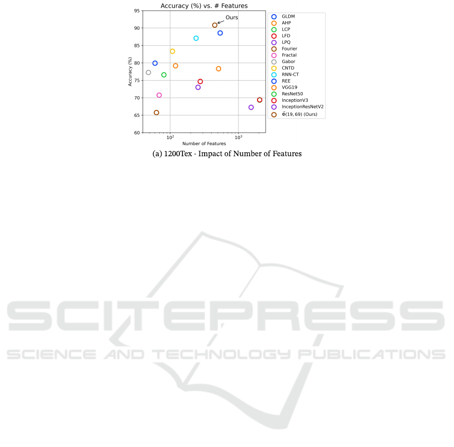
Figure 5: Results for the plant species recognition dataset. (a) Achieved accuracies (%) for the proposed texture descriptor
⃗
Φ(19,69) and other literature methods, comparing the behavior of the obtained accuracy (%) in relation to the number.
posed texture descriptor with the
⃗
Φ(19,69) configu-
ration against other literature methods. Notably, our
approach outperformed all compared methods by a
considerable margin. Specifically, our texture rep-
resentation achieved an accuracy of 90.83%, while
the second-best method, REE (Fares et al., 2024),
achieved 88.58%, representing an improvement of
2.25% and resulting in 27 additional correctly classi-
fied images. Furthermore, our approach achieved the
highest accuracy while maintaining a reduced feature
vector of only 450 attributes, compared to the 540 at-
tributes for the second-best accuracy, representing a
reduction of 16.67% in the feature vector size.
Additionally, we compared our approach against
deep convolutional neural networks. Notably, our ap-
proach demonstrated accuracy improvements of up
to 12.50% compared to the best DCNN accuracy of
78.33% achieved by VGG19 (Simonyan and Zisser-
man, 2014). The inefficiency of these DCNNs in this
dataset may be attributed to two factors. First, the fo-
liar surfaces in this dataset present some level of illu-
mination variation, posing a challenge for the DCNN
architectures. Second, the large feature vectors pro-
duced, even larger than the dataset size, may cause the
curse of dimensionality hindering its performance.
Furthermore, Figure 5(b) shows how the number
of features impacts the accuracy. Notably, methods
with very low (< 100) or very high (> 600) number
of features attain inadequate performance, whereas
the methods ranging from 100 to 600 attributes at-
tain promising results, such as ours. This further re-
inforces the sensitivity that this dataset has to the fea-
ture vector size, thus showing that a moderate number
of attributes is more appropriate for achieving higher
classification accuracies when building a texture rep-
resentation approach.
4 CONCLUSIONS
This paper proposes a new texture representation ap-
proach that uses parameter-free micro-graph mod-
eling, allowing for more effective capture of fine-
grained details in image textures. From these micro-
graphs, we extract topological measures to reveal di-
verse and invariant textural patterns within the image.
These measures are then encoded using a random-
ized neural network in the network’s learned weights,
and we use the statistical summarization of the these
weights as texture representation. The results demon-
strate that the proposed approach is highly discrimi-
native, surpassing several classical and deep learning-
based approaches. Moreover, it outperformed other
graph-based methods as well, highlighting the effec-
tiveness of the micro-graph modeling.
To demonstrate the applicability of our approach,
we also tested it on the challenging task of Brazil-
ian plant species identification using leaf surfaces, in
which it outperformed other methods by a signifi-
cant margin. Therefore, these findings further high-
light the potential of combining micro-graph model-
ing with randomized neural network for robust tex-
ture representation, providing valuable insights to the
fields of computer vision and pattern recognition. As
future work, our method can be adapted for color-
texture and multi-scale analysis, further expanding its
applicability.
ACKNOWLEDGEMENTS
R. T. Fares acknowledges support from FAPESP
(grant #2024/01744-8), L. C. Ribas acknowledges
support from FAPESP (grants #2023/04583-2 and
Exploring Local Graphs via Random Encoding for Texture Representation Learning
207

2018/22214-6). This study was financed in part by
the Coordenac¸
˜
ao de Aperfeic¸oamento de Pessoal de
N
´
ıvel Superior - Brasil (CAPES).
REFERENCES
Abdelmounaime, S. and Dong-Chen, H. (2013). New
brodatz-based image databases for grayscale color and
multiband texture analysis. International Scholarly
Research Notices, 2013.
Backes, A. R., Casanova, D., and Bruno, O. M. (2009).
Plant leaf identification based on volumetric fractal
dimension. International Journal of Pattern Recog-
nition and Artificial Intelligence, 23(06):1145–1160.
Backes, A. R., Casanova, D., and Bruno, O. M. (2012).
Color texture analysis based on fractal descriptors.
Pattern Recognition, 45(5):1984–1992.
Backes, A. R., Casanova, D., and Bruno, O. M.
(2013a). Texture analysis and classification: A com-
plex network-based approach. Information Sciences,
219:168–180.
Backes, A. R., Casanova, D., and Bruno, O. M.
(2013b). Texture analysis and classification: A com-
plex network-based approach. Information Sciences,
219:168–180.
Borzooei, S., Scabini, L., Miranda, G., Daneshgar, S., De-
blieck, L., Bruno, O., De Langhe, P., De Baets, B.,
Nopens, I., and Torfs, E. (2024). Evaluation of acti-
vated sludge settling characteristics from microscopy
images with deep convolutional neural networks and
transfer learning. Journal of Water Process Engineer-
ing, 64:105692.
Brodatz, P. (1966). Textures: A photographic album for
artisters and designerss. Dover Publications.
Calvetti, D., Morigi, S., Reichel, L., and Sgallari, F. (2000).
Tikhonov regularization and the L-curve for large dis-
crete ill-posed problems. Journal of Computational
and Applied Mathematics, 123(1):423 – 446.
Cover, T. M. (1965). Geometrical and statistical properties
of systems of linear inequalities with applications in
pattern recognition. IEEE Transactions on Electronic
Computers, EC-14(3):326–334.
Deng, J., Dong, W., Socher, R., Li, L.-J., Li, K., and Fei-
Fei, L. (2009). Imagenet: A large-scale hierarchical
image database. In 2009 IEEE conference on com-
puter vision and pattern recognition, pages 248–255.
Ieee.
Fares, R. T. and Ribas, L. C. (2024). A new approach
to learn spatio-spectral texture representation with
randomized networks: Application to brazilian plant
species identification. In International Conference on
Engineering Applications of Neural Networks, pages
435–449. Springer.
Fares, R. T., Vicentim, A. C. M., Scabini, L., Zielinski,
K. M., Jennane, R., Bruno, O. M., and Ribas, L. C.
(2024). Randomized encoding ensemble: A new ap-
proach for texture representation. In 2024 31st Inter-
national Conference on Systems, Signals and Image
Processing (IWSSIP), pages 1–8. IEEE.
Florindo, J. B. and Bruno, O. M. (2012). Fractal descriptors
based on Fourier spectrum applied to texture analysis.
Physica A: statistical Mechanics and its Applications,
391(20):4909–4922.
Guo, Y., Zhao, G., and Pietik
¨
ainen, M. (2011). Texture clas-
sification using a linear configuration model based de-
scriptor. In BMVC, pages 1–10. Citeseer.
Guo, Z., Zhang, L., and Zhang, D. (2010a). A completed
modeling of local binary pattern operator for texture
classification. IEEE Transactions on Image Process-
ing, 19(6):1657–1663.
Guo, Z., Zhang, L., and Zhang, D. (2010b). Rotation in-
variant texture classification using lbp variance (lbpv)
with global matching. Pattern recognition, 43(3):706–
719.
Haralick, R. M. (1979). Statistical and structural approaches
to texture. Proceedings of the IEEE, 67(5):786–804.
He, K., Zhang, X., Ren, S., and Sun, J. (2016). Deep resid-
ual learning for image recognition. In Proceedings of
the IEEE conference on computer vision and pattern
recognition, pages 770–778.
Huang, G.-B., Zhu, Q.-Y., and Siew, C.-K. (2006). Extreme
learning machine: Theory and applications. Neuro-
computing, 70(1):489–501.
Jagadeesh, A. V. and Gardner, J. L. (2022). Texture-
like representation of objects in human visual cor-
tex. Proceedings of the National Academy of Sciences,
119(17):e2115302119.
Kannala, J. and Rahtu, E. (2012). Bsif: Binarized statistical
image features. In Pattern Recognition (ICPR), 2012
21st International Conference on, pages 1363–1366.
IEEE.
Kruper, J., Richie-Halford, A., Benson, N. C., Caffarra,
S., Owen, J., Wu, Y., Egan, C., Lee, A. Y., Lee,
C. S., Yeatman, J. D., et al. (2024). Convolutional
neural network-based classification of glaucoma us-
ing optic radiation tissue properties. Communications
Medicine, 4(1):72.
Maani, R., Kalra, S., and Yang, Y.-H. (2013). Noise ro-
bust rotation invariant features for texture classifica-
tion. Pattern Recognition, 46(8):2103–2116.
Manjunath, B. S. and Ma, W.-Y. (1996). Texture features
for browsing and retrieval of image data. IEEE Trans-
actions on pattern analysis and machine intelligence,
18(8):837–842.
Moore, E. H. (1920). On the reciprocal of the general al-
gebraic matrix. Bulletin of American Mathematical
Society, pages 394–395.
Ojala, T., M
¨
aenp
¨
a
¨
a, T., Pietik
¨
ainen, M., Viertola, J.,
Kyll
¨
onen, J., and Huovinen, S. (2002a). Outex - new
framework for empirical evaluation of texture analy-
sis algorithms. Object recognition supported by user
interaction for service robots, 1:701–706 vol.1.
Ojala, T., Pietik
¨
ainen, M., and M
¨
aenp
¨
a
¨
a, T. (2002b). Mul-
tiresolution gray-scale and rotation invariant texture
classification with local binary patterns. Pattern Anal-
ysis and Machine Intelligence, IEEE Transactions on,
24(7):971–987.
Ojansivu, V. and Heikkil
¨
a, J. (2008). Blur insensitive tex-
ture classification using local phase quantization. In
VISAPP 2025 - 20th International Conference on Computer Vision Theory and Applications
208

International conference on image and signal process-
ing, pages 236–243. Springer.
Pao, Y.-H., Park, G.-H., and Sobajic, D. J. (1994). Learning
and generalization characteristics of the random vec-
tor functional-link net. Neurocomputing, 6(2):163–
180.
Pao, Y.-H. and Takefuji, Y. (1992). Functional-link net com-
puting: theory, system architecture, and functionali-
ties. Computer, 25(5):76–79.
Penrose, R. (1955). A generalized inverse for matrices.
Mathematical Proceedings of the Cambridge Philo-
sophical Society, 51(3):406–413.
Ribas, L. C., S
´
a Junior, J. J. M., Scabini, L. F., and Bruno,
O. M. (2020). Fusion of complex networks and ran-
domized neural networks for texture analysis. Pattern
Recognition, 103:107189.
Ribas, L. C., Scabini, L. F., Condori, R. H., and Bruno,
O. M. (2024a). Color-texture classification based
on spatio-spectral complex network representations.
Physica A: Statistical Mechanics and its Applications,
page 129518.
Ribas, L. C., Scabini, L. F., de Mesquita S
´
a Junior, J. J., and
Bruno, O. M. (2024b). Local complex features learned
by randomized neural networks for texture analysis.
Pattern Analysis and Applications, 27(1):23.
S
´
a Junior, J. J. M. and Backes, A. R. (2016). ELM based
signature for texture classification. Pattern Recogni-
tion, 51:395–401.
Schmidt, W., Kraaijveld, M., and Duin, R. (1992). Feed-
forward neural networks with random weights. In
Proceedings., 11th IAPR International Conference on
Pattern Recognition. Vol.II. Conference B: Pattern
Recognition Methodology and Systems, pages 1–4.
Simonyan, K. and Zisserman, A. (2014). Very deep convo-
lutional networks for large-scale image recognition.
Song, T., Li, H., Meng, F., Wu, Q., and Cai, J. (2018).
Letrist: Locally encoded transform feature histogram
for rotation-invariant texture classification. IEEE
Transactions on Circuits and Systems for Video Tech-
nology, 28(7):1565–1579.
Szegedy, C., Ioffe, S., Vanhoucke, V., and Alemi, A. A.
(2017). Inception-v4, inception-resnet and the impact
of residual connections on learning. In Thirty-First
AAAI Conference on Artificial Intelligence.
Szegedy, C., Vanhoucke, V., Ioffe, S., Shlens, J., and Wo-
jna, Z. (2016). Rethinking the inception architecture
for computer vision. In Proceedings of the IEEE con-
ference on computer vision and pattern recognition,
pages 2818–2826.
Tikhonov, A. N. (1963). On the solution of ill-posed prob-
lems and the method of regularization. Dokl. Akad.
Nauk USSR, 151(3):501–504.
Weszka, J. S., Dyer, C. R., and Rosenfeld, A. (1976). A
comparative study of texture measures for terrain clas-
sification. IEEE transactions on Systems, Man, and
Cybernetics, (4):269–285.
Xu, Z., Jiang, W., and Geng, J. (2024). Texture-aware
causal feature extraction network for multimodal re-
mote sensing data classification. IEEE Transactions
on Geoscience and Remote Sensing.
Zhu, Z., You, X., Chen, C. P., Tao, D., Ou, W., Jiang,
X., and Zou, J. (2015). An adaptive hybrid pattern
for noise-robust texture analysis. Pattern Recognition,
48(8):2592–2608.
Zielinski, K. M. C., Ribas, L. C., Scabini, L. F. S.,
and Bruno, O. M. (2022). Complex texture fea-
tures learned by applying randomized neural network
on graphs. In Eleventh International Conference
on Image Processing Theory, Tools and Applications
(IPTA), Salzburg, Austria, pages 1–6.
Exploring Local Graphs via Random Encoding for Texture Representation Learning
209