Volumetric Color-Texture Representation for Colorectal Polyp
Classification in Histopathology Images
Ricardo T. Fares
a
and Lucas C. Ribas
b
S
˜
ao Paulo State University, Institute of Biosciences, Humanities and Exact Sciences, S
˜
ao Jos
´
e do Rio Preto, SP, Brazil
Keywords:
Color-Texture, Texture Representation Learning, Randomized Neural Network.
Abstract:
With the growth of real-world applications generating numerous images, analyzing color-texture information
has become essential, especially when spectral information plays a key role. Currently, many randomized neu-
ral network texture-based approaches were proposed to tackle color-textures. However, they are integrative
approaches or fail to achieve competitive processing time. To address these limitations, this paper proposes a
single-parameter color-texture representation that captures both spatial and spectral patterns by sliding volu-
metric (3D) color cubes over the image and encoding them with a Randomized Autoencoder (RAE). The key
idea of our approach is that simultaneously encoding both color and texture information allows the autoen-
coder to learn meaningful patterns to perform the decoding operation. Hence, we employ as representation
the flattened decoder’s learned weights. The proposed approach was evaluated in three color-texture bench-
mark datasets: USPtex, Outex, and MBT. We also assessed our approach in the challenging and important
application of classifying colorectal polyps. The results show that the proposed approach surpasses many
literature methods, including deep convolutional neural networks. Therefore, these findings indicate that our
representation is discriminative, showing its potential for broader applications in histological images and pat-
tern recognition tasks.
1 INTRODUCTION
The advancement of numerous image acquisi-
tion techniques has continuously enabled various
real-world applications to acquire colored images.
Largely, several of these applications, such as im-
age retrieval (Liu and Yang, 2023), face recognition
(Li et al., 2024), defect recognition (Su et al., 2024),
and medical diagnosis (Rangaiah et al., 2025) rely on
texture descriptors. Texture description of an image
consists in leveraging one of the most important low-
level visual cues, the texture, to obtain a sequence of
real numbers describing the image with the purpose
of performing pattern recognition tasks.
In this context, to enable the recognition of texture
images, several texture descriptors have been devel-
oped and advanced over the years through techniques
such as those based on local binary patterns (Ojala
et al., 2002b; Guo et al., 2010; Hu et al., 2024), which
encode pixel neighborhoods using the central pixel lu-
minance as a threshold; graph-based methods (Backes
a
https://orcid.org/0000-0001-8296-8872
b
https://orcid.org/0000-0003-2490-180X
et al., 2013; Scabini et al., 2019), which apply com-
plex network theory to describe structural patterns
in images using graph measures; and mathematical
approaches that used the Bouligand-Minkowski frac-
tal dimension (Backes et al., 2009). Although these
methods are highly significant as they lay the founda-
tion for the development of newer and more powerful
approaches, they may fail to achieve strong perfor-
mance on more complex images, as those may not be
adequately described using only textural attributes.
In this sense, with the increasing attention of the
research community in deep-learning and with the
outstanding results achieved by AlexNet (Krizhevsky
et al., 2012) in the ImageNet (Deng et al., 2009) chal-
lenge, there was a shift in focus to learning-based
strategies, leading to the development of various CNN
architectures, such as the VGG (Simonyan and Zisser-
man, 2014), ResNet (He et al., 2016) and DenseNet
(Huang et al., 2017) families.
Nevertheless, deep neural networks pose some
challenges, such as their need for large training data
and significant computational cost due to the training
of their large number of parameters. In relation to
large training data issues, numerous recent method-
210
Fares, R. T. and Ribas, L. C.
Volumetric Color-Texture Representation for Colorectal Polyp Classification in Histopathology Images.
DOI: 10.5220/0013315800003912
Paper published under CC license (CC BY-NC-ND 4.0)
In Proceedings of the 20th International Joint Conference on Computer Vision, Imaging and Computer Graphics Theory and Applications (VISIGRAPP 2025) - Volume 3: VISAPP, pages
210-221
ISBN: 978-989-758-728-3; ISSN: 2184-4321
Proceedings Copyright © 2025 by SCITEPRESS – Science and Technology Publications, Lda.

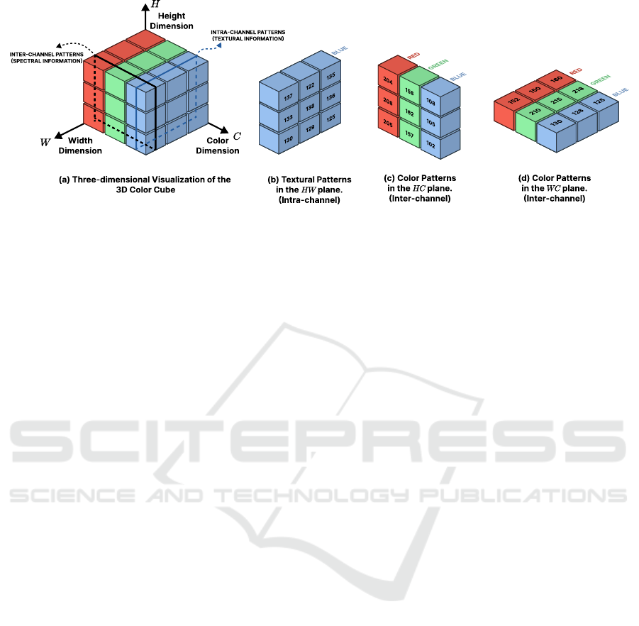
Figure 1: Illustration of the 3D color cubes used to capture spatial and cross-channel color information in the color-texture
image. (a) Three-dimensional view of the 3D color cube. (b) Extracted textural patterns in the HW plane. (c) Color patterns
observed in the HC plane. (d) Color patterns observed in the WC plane.
ologies apply data augmentation. However, data aug-
mentation must be carefully selected to not alter the
sample label (Wang et al., 2021). On the other hand,
although significant computational cost can be soft-
ened by using model compression through quantiza-
tion or pruning, there may be some loss of accuracy
during training (Marin
´
o et al., 2023).
In this sense, many recent texture representation
methods used randomized neural networks (S
´
a Junior
and Backes, 2016; Ribas et al., 2024a; Fares et al.,
2024). These networks offer simplicity, low compu-
tational costs, and have proven to obtain satisfactory
results in pattern recognition applications. In these
studies, the authors train a randomized neural network
for each image and conduct a post-processing of the
learned weights of the randomized neural network,
which carries valuable information. Despite achiev-
ing good results, many color-texture representation
methods focus on spatial patterns or apply separate
grayscale analysis to each channel, overlooking spec-
tral and cross-channel information, thus losing valu-
able color details. Furthermore, those that perform
spatial-spectral analysis fail in achieving competitive
feature extraction processing time.
To address these limitations, in this paper, we pro-
pose a fast single-parameter color-texture represen-
tation based on a randomized autoencoder that si-
multaneously encodes texture and color information
(spatio-spectral) using volumetric (3D) color cubes.
Initially, for a given 3-channel we assemble the input
feature matrix by flattening 3D color cubes of dimen-
sion 3×3 ×3 over the entire image (Fig. 1), capturing
both spatio and spectral information. Following this,
we apply this feature matrix of a single image to a ran-
domized autoencoder that randomly projects the input
data into another dimensional space, and learns how
to reconstruct them back to the input space, thereby
learning the meaningful textural and color character-
istics to perform it. Thus, we use as color-texture
representation the flattening of the decoder’s learned
weights of the randomized autoencoder. Overall, the
major contributions of our work are:
• Simple, fast and low cost approach that learns the
representation using a single instance due to use
of randomized autoencoders.
• A texture representation that simultaneously cap-
tures both texture and color patterns.
• A color-texture representation that outperforms
several texture-only literature methods in the ap-
plication of classifying colorectal polyps.
This paper is organized as follows: Section 2
presents the proposed color-texture representation ap-
proach. Section 3 presents the experimental setup, the
results, and comparisons with other literature meth-
ods, and Section 4 concludes this paper.
2 PROPOSED APPROACH
2.1 Randomized Neural Networks
Randomized neural networks (RNN) consist of a sin-
gle fully-connected hidden layer, with the weights
randomly generated from a probability distribution
(e.g. normal or uniform) (Huang et al., 2006; Pao
and Takefuji, 1992; Pao et al., 1994; Schmidt et al.,
1992). Their simplicity arises from the use of a single
hidden layer, and the learning phase is efficient due to
the output layer weights being computed via a closed-
form solution. The network’s primary goal is to non-
linearly random project the input data into another di-
mensional space to enhance the linear separability of
the data, as stated in Cover’s theorem (Cover, 1965).
The weights of the output layer are then learned by
Volumetric Color-Texture Representation for Colorectal Polyp Classification in Histopathology Images
211

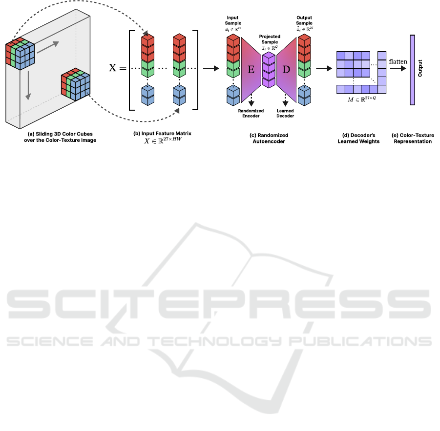
Figure 2: Illustration of the proposed color-texture methodology. (a) Sliding 3D color cubes over the color-texture image to
build the input feature matrix. (b) The input feature matrix. (c) Randomized autoencoder to randomly project this matrix. (d)
Decoder’s learned weights. (e) Proposed color-texture representation.
fitting these linearly enhanced data using the least-
squares method.
Formally, let X ∈ R
p×N
and Y ∈ R
r×N
be the in-
put and output feature matrices, respectively. The in-
put feature matrix is composed by N input feature
vectors of dimension p, whereas the output feature
matrix consists of N output feature vectors of dimen-
sion r. Subsequently, a probability distribution p(x
x
x)
is employed to generate the random weight matrix
W ∈ R
Q×(p+1)
, with the first column being the bias’
weights, and where Q is the number of neurons in the
hidden layer, or more specifically the dimension of
the latent space.
Following this, we append a value −1 at the top
of every column of X , linking the input feature vec-
tors with the bias’ weights. From this, the randomly
projected input feature vectors can be computed by
Z = φ(W X), where each column of Z consists of the
projected feature vector, and φ is the sigmoid func-
tion. After obtaining the projected matrix Z, a −1 is
appended to the top of each projected feature vector
to connect to the bias weight of the output neurons.
Hence, the output layer weights (M) of the ran-
domized neural network are computed using the fol-
lowing closed-form solution, which consists in a brief
sequence of matrix operations:
M = Y Z
T
(ZZ
T
+ λI)
−1
, (1)
where the term (ZZ
T
+ λI)
−1
represents the regu-
larized Moore-Penrose pseudoinverse (Moore, 1920;
Penrose, 1955) with Tikhonov’s regularization
(Tikhonov, 1963; Calvetti et al., 2000). This regu-
larization is used to avoid issues related to the inver-
sion of near-singular matrices. Finally, the random-
ized neural network may be employed as a random-
ized autoencoder (RAE) by setting Y = X.
2.2 VCTex: Volumetric Color-Texture
Representation
In this paper, we propose to use as color-texture rep-
resentation the flattened decoder’s learned weights of
a randomized autoencoder trained with simultaneous
key information of color and textural patterns. These
patterns are extracted using 3D color cubes that slide
across the color-texture image, effectively capturing
the color-textural information.
To build the color-texture representation, we first
build the input feature matrix X. For this, let I ∈
R
3×H×W
be any RGB image, we assemble X by flat-
tening 3D cubes of size 3 × 3 × 3 that slide over each
pixel in the green channel and horizontally concate-
nate them. Positioning the cube in the green channel
allows us to capture information from both red and
blue channels. Consequently, each cube captures spa-
tial patterns of each channel (each 3×3 window along
the color depth) as well as cross-channel color (spec-
tral) information, as illustrated in Figure 1.
After assembling the input feature matrix, we
build the random weight matrix, W , to encode the
input data. To ensure that our method consistently
produces the same color-texture representation for the
same image on every run, the random weights are kept
fixed, ensuring reproducibility. To this end, we em-
ploy the Linear Congruent Generator (LCG) to ob-
tain pseudorandom values for the matrix W using the
recurrent formula: V (n + 1) = (aV (n) + b) mod c,
where V has length ℓ = Q ·(p+1), and initial parame-
ters set to V (0) = ℓ+1,a = ℓ+2, b = ℓ+3, and c = ℓ
2
.
Following this, V is standardized, and W results from
turning the vector V into a matrix of size Q × (p + 1).
Subsequently, X is applied to a randomized au-
toencoder, and the decoder’s learned weights, M, are
computed using the Equation 1. These weights con-
VISAPP 2025 - 20th International Conference on Computer Vision Theory and Applications
212

tain meaningful spatial and cross-channel related in-
formation, as they are trained to decode the randomly
encoded color-texture information provided by the 3D
sliding cubes. Thus, we define a partial color-texture
representation by flattening these learned weights,
formulated as:
⃗
Θ(Q) = flatten(X Z
T
(ZZ
T
+ λI)
−1
), (2)
where Z, λ and I are the projected matrix, the regu-
larization parameter and the identity matrix, all previ-
ously defined in Section 2.1.
Finally, given that the partial representation
⃗
Θ(Q)
relies only on the value of Q, we can enhance our
texture representation by combining the learned rep-
resentations across different Q values. Each distinct
Q characterizes the image uniquely, capturing distinct
aspects of color and texture. Hence, we define our
proposed color-texture representation as:
⃗
Ω(Q) = concat(
⃗
Θ(Q
1
),
⃗
Θ(Q
2
),...,
⃗
Θ(Q
m
)), (3)
where Q = (Q
1
,Q
2
,...,Q
m
).
3 EXPERIMENTS AND RESULTS
3.1 Experimental Setup
In order to evaluate the proposed approach, we used
the accuracy metric obtained by employing Linear
Discriminant Analysis (LDA) as classifier with the
leave-one-out cross-validation strategy. LDA was
chosen due to its simplicity, emphasizing that the ro-
bustness of the proposed approach stems from the
extracted features. Furthermore, we employed three
color-texture benchmark datasets with distinct char-
acteristics and variations:
• USPtex (Backes et al., 2012): This dataset is com-
posed by 2922 natural texture samples of 128 ×
128 pixels, distributed among 191 classes, each
having 12 images.
• Outex (Ojala et al., 2002a): Outex consists of
1360 samples partitioned into 68 classes, each
having 20 samples of size 128 × 128 pixels.
• MBT (Abdelmounaime and Dong-Chen, 2013):
MBT is composed by 2464 texture samples that
exhibit distinct intra-band and inter-band spatial
patterns. These samples are grouped into 154
classes, each having 16 images of 160 × 160 pix-
els.
Finally, we compared our proposed approach with
several classical and learning-based approaches re-
ported in the literature. The compared methods in-
clude: GLCM (Haralick, 1979), Fourier (Weszka
et al., 1976), Fractal (Backes et al., 2009), LBP (Ojala
et al., 2002b), LPQ (Ojala et al., 2002b), LCP (Guo
et al., 2011), AHP (Zhu et al., 2015), BSIF (Kannala
and Rahtu, 2012), CLBP (Guo et al., 2010), LETRIST
(Song et al., 2017), LGONBP (Song et al., 2020a),
SWOBP (Song et al., 2020b), RNN-RGB (S
´
a Ju-
nior et al., 2019), SSR (Ribas et al., 2024a), VGG11
(Simonyan and Zisserman, 2014), ResNet18 and
ResNet50 (He et al., 2016), and DenseNet121 (Huang
et al., 2017), and InceptionResNetV2 (Szegedy et al.,
2017).
3.2 Parameter Investigation
One of the key advantages of our approach is that it
depends solely on a single-type of parameter, which
is the number of hidden neurons (Q). This simplicity
allows the descriptor to be easily assessed or adapted
for other computer vision tasks. Here, we evaluated
the proposed descriptor on the three presented tex-
ture benchmarks. Specifically, we analyzed the be-
havior of the classification accuracy (%) of the pro-
posed texture representation
⃗
Θ(Q) for each dataset,
considering the numbers of hidden neurons within the
set {1, 5, 9, 13, 17, 21, 25, 29}, starting from 1 up to 29
in steps of 4.
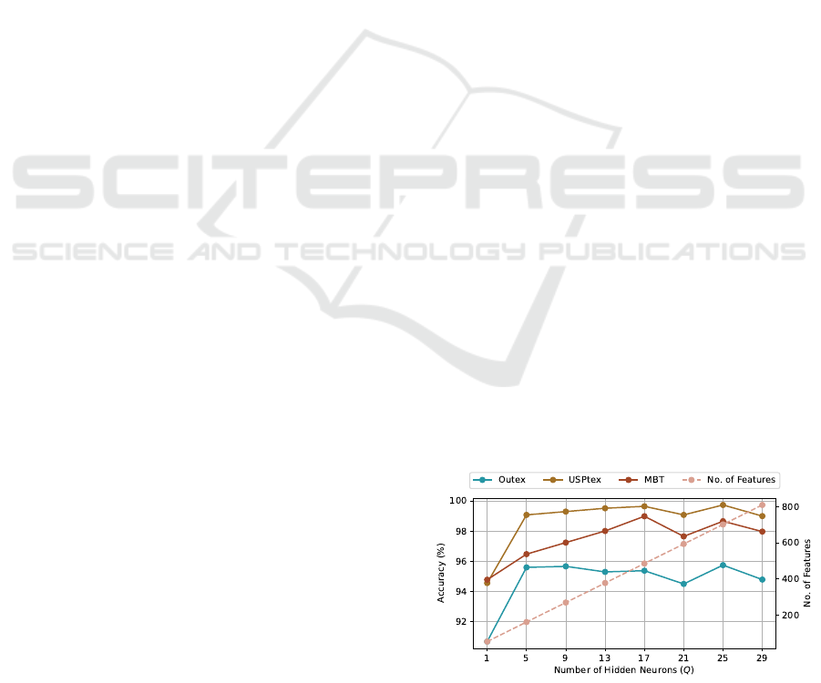
Figure 3 illustrates that accuracy increases across
all datasets as the number of hidden neurons rises,
suggesting a positive impact of increasing the number
of hidden neurons, Q, of the randomized autoencoder.
Nevertheless, at Q = 21, the accuracy drops across the
datasets, and beyond this point, the accuracy begins to
fluctuate, indicating a state of relative stability, partic-
ularly for the USPtex and MBT datasets. In summary,
these observations imply that our approach benefits
from higher-dimensional projections, but overly high
dimensions may not be ideal. This behavior could be
attributed to the increase in the number of features, to
which some datasets, such as Outex, are more sensi-
tive.
Figure 3: Dynamics of the classification accuracy rate (%)
as the number of hidden neurons (Q) rises, for the proposed
texture descriptor
⃗
Θ(Q).
Volumetric Color-Texture Representation for Colorectal Polyp Classification in Histopathology Images
213

To mitigate fluctuations in the accuracies with a
single number of hidden neurons, we combine the
texture representations from distinct hidden neurons
Q
1
and Q
2
. This strategy leverages the diverse tex-
tural patterns learned by each neuron to create an
even more robust texture descriptor, previously de-
fined as
⃗
Ω(Q
1
,Q
2
). We assessed this descriptor by
analyzing the accuracy achieved for different com-
binations of Q
1
and Q
2
of hidden neurons, where
Q
1
,Q
2
∈ {1,5,9,13,17,21,25,29}, with Q
1
< Q
2
.
Table 1 presents the results of the descriptor
⃗
Ω(Q
1
,Q
2
) across all datasets, along with the aver-
age accuracy. We observed that combining learned
representation by varying the number of hidden neu-
rons leads to better accuracy. This finding aligns
with other RNN-based investigations, such as (Ribas
et al., 2024b; Fares and Ribas, 2024), which showed
that combining representations from different latent
spaces positively impacts accuracy. This occurs be-
cause each learned feature vector uniquely charac-
terizes the textural patterns by learning how to re-
construct them from distinct Q
1
- and Q
2
-dimensional
spaces.
Table 1: Accuracy rates (%) of the proposed descriptor
⃗
Ω(Q
1
,Q
2
), for each dataset, and for every possible com-
bination of Q
1
and Q
2
. Bold emphasizes the result with
highest average accuracy.
(Q
1
,Q
2
) # Features USPtex Outex MBT Avg.
(01, 05) 216 99.0 95.7 97.2 97.3
(01, 09) 324 99.5 96.1 97.9 97.8
(01, 13) 432 99.5 95.4 98.2 97.7
(01, 17) 540 99.6 95.8 98.9 98.1
(01, 21) 648 99.2 94.3 97.7 97.1
(01, 25) 756 99.7 95.9 98.7 98.1
(01, 29) 864 99.1 94.9 98.3 97.4
(05, 09) 432 99.7 96.0 97.3 97.7
(05, 13) 540 99.7 95.2 97.8 97.6
(05, 17) 648 99.6 96.0 99.1 98.2
(05, 21) 756 99.6 95.2 97.9 97.6
(05, 25) 864 99.6 95.2 98.7 97.8
(05, 29) 972 99.4 96.0 98.3 97.9
(09, 13) 648 99.7 96.1 97.9 97.9
(09, 17) 756 99.7 94.9 98.9 97.8
(09, 21) 864 99.5 94.9 98.3 97.6
(09, 25) 972 99.7 94.9 98.7 97.8
(09, 29) 1080 99.6 95.7 98.4 97.9
(13, 17) 864 99.7 94.9 98.9 97.8
(13, 21) 972 99.7 95.0 98.6 97.8
(13, 25) 1080 99.7 93.8 98.7 97.4
(13, 29) 1188 99.7 95.7 98.4 97.9
(17, 21) 1080 99.7 95.1 99.2 98.0
(17, 25) 1188 99.7 93.2 98.9 97.3
(17, 29) 1296 99.7 95.4 99.2 98.1
(21, 25) 1296 99.7 94.6 98.9 97.8
(21, 29) 1404 99.4 94.8 98.6 97.6
(25, 29) 1512 99.7 95.2 98.9 98.0
Furthermore, although some combinations do not
always guarantee improved accuracy, these excep-
tions could be attributed to the large feature vector
sizes, where some datasets such as Outex are more
sensitive. This effect is clearly visible in the Ou-
tex column, which shows a decline, mainly after the
configuration
⃗
Ω(09,13), whereas USPtex and MBT
maintain a steady performance. Consequently, this
trend reveals a peak in the achieved average accuracy,
indicating a point where the descriptor offers a robust
characterization across all datasets.
Finally, based on these findings, we observed that
the configuration
⃗
Ω(05,17) achieved the highest av-
erage accuracy of 98.2%, making it the most robust
version of the proposed approach. Therefore, we se-
lected this configuration for comparison against other
methods in the literature.
3.3 Comparison and Discussions
In this section, we compared the previously selected
configuration,
⃗
Ω(05,17), of our proposed texture ap-
proach with methods from the literature described
in Section 3.1. The compared methods were evalu-
ated using the same experimental setup: Linear Dis-
criminant Analysis (LDA) with leave-one-out cross-
validation, using the accuracy metric for comparison.
Table 2 presents the results obtained by our
method and others in the literature. The results
highlight that our approach outperformed all com-
pared methods on the USPtex and MBT datasets and
achieved the second-best performance on the Ou-
tex dataset, surpassed only by SSR (Ribas et al.,
2024a). Specifically, when comparing our approach
with the classical and RNN-based methods, ranging
from GLCM to SSR, our approach not only outper-
formed SSR by 0.6% on the USPtex dataset but also
achieved an accuracy of 99.1% on the MBT dataset,
standing out as the only method to surpass the 99%
accuracy mark. Furthermore, it is noteworthy that our
proposed approach also surpassed other RNN-based
methods, such as SSR and RNN-RGB, highlighting
the effectiveness of using 3D color cubes to model the
multi-channel textural patterns and randomly encode
them.
In addition, to provide a broader quantitative anal-
ysis, we compared our approach with various deep
convolutional neural networks (DCNNs) described in
Section 3.1. These networks were used as feature ex-
tractors, employing pre-trained models on ImageNet.
Furthermore, to prevent excessively large feature vec-
tor sizes that could lead to dimensionality issues, fea-
tures are extracted by applying Global Average Pool-
ing (GAP) to the last convolutional layer, as also done
in other investigations, such as (Ribas et al., 2024b).
VISAPP 2025 - 20th International Conference on Computer Vision Theory and Applications
214

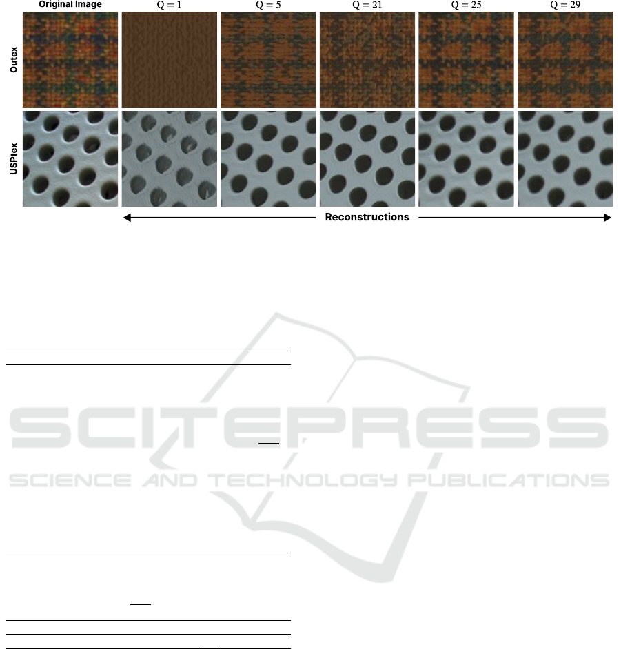
Figure 4: Plot of the original image and their reconstructions for distinct number of hidden neurons (Q). As Q increases the
reconstruction quality also improves, with Q = 25 being with the most quality from a visual inspection. The quality of the
reconstructions suggests that the decoder’s learned weights captured the essential texture information.
Table 2: Comparison of the classification accuracy rates (%)
of the proposed texture descriptor
⃗
Ω(Q
1
,Q
2
) against other
methods in the literature on three color-texture datasets.
Bold denotes the best result, and underline the second best.
Method USPTex Outex MBT
GLCM integrative 95.9 91.1 97.4
Fourier integrative 91.6 85.8 96.3
Fractal integrative 95.0 86.8 97.0
LBP integrative 90.2 82.4 96.6
LPQ integrative 90.4 80.1 95.7
LCP integrative 96.9 90.7 98.5
AHP integrative 98.7 93.4 98.1
BSIF integrative 82.9 77.9 97.9
CLBP integrative 97.4 89.6 98.2
LGONBP (gray-level) 83.3 83.5 74.2
LETRIST (gray-level) 92.4 82.8 79.1
SWOBP 97.0 79.3 88.3
RNN-RGB 98.4 94.8 −
SSR 99.0 96.8 98.0
VGG11 99.3 89.9 93.8
ResNet18 98.7 86.7 90.8
ResNet50 89.4 86.8 85.6
DenseNet121 99.4 84.7 94.1
InceptionResNetV2 96.7 82.4 89.5
Proposed Method
VCTex 99.6 96.0 99.1
In this context, Table 2 shows that our proposed
method outperformed the DCNN-based approaches
across all datasets. Specifically, our approach stands
out in both the Outex and MBT datasets, achieving ac-
curacies of 96.0% and 99.1%, respectively. These re-
sults correspond to increases of 6.1% on Outex com-
pared to VGG11 (89.9%) and an increase of 5.0%
on MBT compared to DenseNet121 (94.1%). These
findings suggest that DCNNs face some challenges
in characterizing texture on the Outex and MBT,
potentially due to micro-texture variations in Outex
and inter- and intra-band spatial variations in MBT,
whereas our proposed approach efficiently character-
izes it. Conversely, although our approach achieved
only slight accuracy improvements on USPtex, in
comparison to VGG11 (99.3%) and DenseNet121
(99.4%), it still outperformed the compared DC-
NNs, demonstrating that our method is just as robust
for texture characterization as transferred knowledge
from models pre-trained on millions of images.
To provide a complement to the quantitative anal-
ysis, we assess the qualitative aspect of our approach
by plotting their reconstructions, as illustrated in Fig-
ure 4. Although we do not use the reconstruction error
as a metric for the quantitative aspect of our approach,
since we use the decoder’s learned weights as texture
representation. This figure shows that as the number
of hidden neurons increases, Q, the quality of the re-
construction increases, with Q = 25 the one most re-
sembling the original image, which matched the best
configuration,
⃗
Θ(25), found in Figure 3. These visu-
alizations are important because they show that the in-
formation learned by the decoder’s weights carries in-
sightful textural content, indicating the effectiveness
of the proposed color-texture representation.
Finally, based on these findings, our proposed ap-
proach proved effective in characterizing color tex-
tures, outperforming several hand-engineered meth-
ods and pre-trained deep convolutional neural net-
works. These results indicate the robustness of mod-
eling color and textural patterns by sliding 3D color
cubes over the image and randomly encoding them,
thereby capturing all key color and texture informa-
tion simultaneously, rather than using gray-scale tex-
ture methods applied to each image color channel as
integrative approaches do.
Volumetric Color-Texture Representation for Colorectal Polyp Classification in Histopathology Images
215

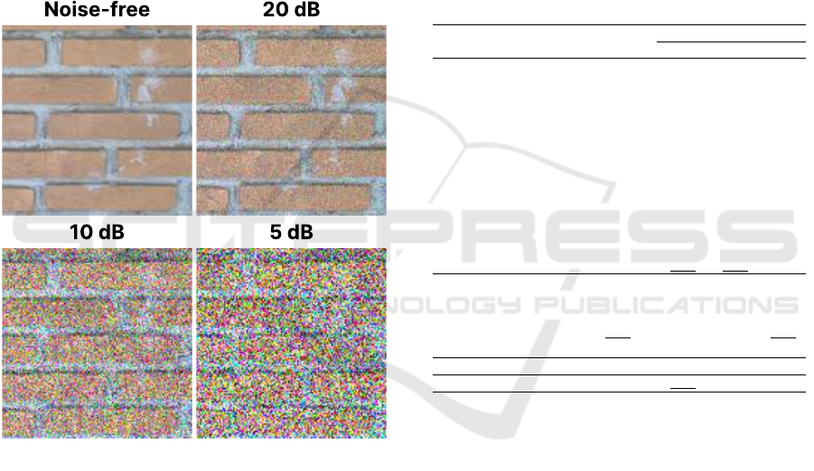
3.4 Noise Robustness Analysis
This section assesses the capacity of the proposed tex-
ture descriptor regarding noise tolerance. Noise in im-
ages is a condition that can happen for some reasons,
such as image equipment acquisition. In this context,
to evaluate the behavior of the proposed technique in
noise conditions, we applied the additive white Gaus-
sian noise (AWGN) to the USPtex dataset with dif-
ferent signal-to-noise ratio (SNR) values specified in
decibel (dB). Specifically, we evaluated the compared
texture descriptors in the noise-free conditions and in
three different SNR ∈ {20, 10, 5}, indicating moder-
ate to high levels of noise. Figure 5 shows the noise-
free and some noisy samples.
Figure 5: Samples of the USPtex (Backes et al., 2012)
dataset in its noise-free condition and with different additive
White Gaussian noise conditions specified by the signal-to-
noise ratio in decibels (dB).
Table 3 exhibits the comparison of the proposed
approach against the compared methods with differ-
ent SNR values. VCTex achieved the best accuracy in
the noise-free condition (99.6%), and the second-best
with 20 dB (97.9%), while DenseNet121 achieved the
highest one (98.8%). For high levels of noise, VCTex
ranked in fourth and fifth for the 10 dB (81.7%) and
5 dB (60.7%) conditions, respectively. These results
indicate that VCTex is tolerant for a moderate level
of noise, and although it did not achieve the highest
accuracies in high level conditions, it remained in the
top five.
Therefore, based on the results, we suspect that
the sensitivity of VCTex in high levels of noise is
due to the direct encoding of image pixel intensities
through 3 × 3 × 3 cubes. Under high-noise condi-
tions, these pixels are significantly modified, leading
the proposed texture representation to encode some of
the noise. This is somehow undesirable for learning a
robust texture representation. This hypothesis is fur-
ther supported by the better noise tolerance demon-
strated by SSR, a method that encodes pixels using
a graph-based model. Consequently, VCTex exhibits
certain limitations when dealing with excessive noise
levels.
Table 3: Comparison of the accuracy rates (%) of the pro-
posed texture descriptor against other literature methods in
distinct additive white Gaussian noise (AWGN) conditions
specified by the signal-to-noise ratio value in decibels (dB).
AWGN
Method Noise-free 20 dB 10 dB 5 dB
GLCM integrative 95.9 91.0 71.6 55.2
Fourier integrative 91.6 85.2 70.4 61.8
Fractal integrative 95.0 73.8 46.4 31.8
LBP integrative 90.2 66.8 32.7 28.2
LPQ integrative 90.4 78.8 43.2 23.7
LCP integrative 96.9 86.8 61.5 51.8
AHP integrative 98.7 90.0 70.5 58.1
BSIF integrative 82.9 76.1 52.1 33.3
CLBP integrative 97.4 42.5 21.0 17.5
LGONBP (gray-level) 92.4 77.7 55.1 35.6
LETRIST (gray-level) 97.0 87.5 64.8 43.1
SWOBP 98.4 86.0 55.4 40.2
SSR 99.0 97.9 86.4 68.8
VGG11 99.3 95.7 71.3 39.1
ResNet18 98.7 96.8 80.1 51.8
ResNet50 89.4 86.3 53.8 34.5
DenseNet121 99.4 98.8 88.9 65.6
InceptionResNetV2 96.7 97.0 85.7 62.0
Proposed Approach
VCTex 99.6 97.9 81.7 60.7
3.5 Computational Efficiency
In this analysis, we investigate how computationally
efficient the proposed approach is against the com-
pared methods in the literature. For this purpose, we
compared the average running time of the feature ex-
traction methods in 100 trials after 10 warm-up trials.
These warm-up trials were employed to prevent some
outlier measurements, such as those caused by cold
start issues. Therefore, doing so allowed us to provide
a more robust and consistent analysis of the results.
To run the processing time measurement experi-
ments, we used a server equipped with a i9-14900KF
processor with 128 GB RAM and a GeForce RTX
4090 24GB GPU, running on the Ubuntu 22.04 op-
erating system. The hand-engineered methods and
SSR were implemented using MATLAB (R2023b),
while the DCNN-based methods and VCTex were
VISAPP 2025 - 20th International Conference on Computer Vision Theory and Applications
216

implemented using Python v3.11.9 and the PyTorch
(Paszke et al., 2019) library v2.4.0.
Table 4 presents the average processing time (in
seconds) for the compared hand-engineered methods.
As shown, our proposed approach (VCTex) achieved
the lowest average processing time of 0.0093 sec-
onds (9.3 ms), exhibiting a very efficient approach.
Further, in comparison, our approach is 1.95× faster
than the second most efficient approach (LBP), and
also achieved superior classification results across all
benchmark datasets as presented in Table 2. Ad-
ditionally, regarding other RNN-based techniques,
such as SSR, our approach demonstrated to be 242×
faster. Here, although SSR uses the RNN architecture
(which is simple and fast), this high cost in processing
time is largely due to the graph-modeling phase.
Table 4: Report of the average processing time (in seconds)
of 100 trials for each compared hand-engineered method
using a 224 × 224 RGB image. Bold denotes the best result,
and underline the second best. Lower values are preferable.
Method CPU Time (s)
GLCM integrative 0.0421 ± 0.0082
Fourier integrative 0.0553 ± 0.0089
Fractal integrative 2.8410 ± 0.0085
LBP integrative 0.0181 ± 0.0075
LPQ integrative 0.2302 ± 0.0154
LCP integrative 0.1176 ± 0.0105
AHP integrative 0.1746 ± 0.0126
BSIF integrative 0.0295 ± 0.0085
CLBP integrative 0.2366 ± 0.0156
LGONBP (gray-level) 0.3839 ± 0.0214
LETRIST (gray-level) 0.0246 ± 0.0035
SWOBP 0.3198 ± 0.0453
SSR 2.2551 ± 0.0971
Proposed Approach
VCTex 0.0093 ± 0.0002
Following this, Table 5 shows the average pro-
cessing time (in seconds) in both CPU and GPU
for the DCNN-based methods in comparison to VC-
Tex. In terms of CPU time, the VCTex achieved
the lowest average processing time (9.3 ms), be-
ing faster than the compared architectures in 2.83×
(VGG11), 1.51× (ResNet18), 2.96× (ResNet50),
57.03× (DenseNet121) and 6.94× (InceptionRes-
NetV2). Conversely, in terms of GPU time, the
lowest average processing time was achieved by
VGG11 with 0.0004 seconds (0.4 ms), and the sec-
ond best was achieved by ResNet18 with 0.0010 sec-
onds (1.0 ms), with our approach ranking in third
with 0.0013 seconds (1.3 ms). Although the VCTex
is slightly slower than ResNet18 and 3.25× slower
than VGG11, our proposed method consistently out-
performed these pre-trained feature extractors in all
the benchmark datasets, thus showing a good balance
between the trade-off of computational efficiency and
accuracy.
Table 5: Report of the average processing time (in seconds)
of 100 trials for each compared DCNN-based method using
a 224 × 224 RGB image. Bold denotes the best result, and
underline the second best. Lower values are preferable.
Time (ms)
Method CPU GPU
VGG11 0.0263 ± 0.0007 0.0004 ± 0.0001
ResNet18 0.0140 ± 0.0007 0.0010 ± 0.0000
ResNet50 0.0275 ± 0.0006 0.0025 ± 0.0000
DenseNet121 0.5304 ± 0.0225 0.0065 ± 0.0000
InceptionResNetV2 0.0645 ± 0.0005 0.0124 ± 0.0001
Proposed Approach
VCTex 0.0093 ± 0.0002 0.0013 ± 0.0000
Therefore, this investigation showed that VCTex
has a high competitive computational performance,
achieving the lowest average processing in CPU time
across all compared methods, and ranking in third in
terms of GPU time. This good performance is largely
due to the employed RNN architecture and the rapid
tensor stride manipulation operations to obtain the
3 × 3 × 3 cubes across every pixel in the image. In
this sense, VCTex presents as a competitive approach
both in terms of accuracy and computational perfor-
mance.
3.6 Classification of Colorectal Polyps
Colorectal cancer (CRC) is the second leading cause
of cancer-related mortality and the third most fre-
quently diagnosed cancer worldwide (Choe et al.,
2024). Thus, early diagnosis is important, as it allows
for early treatment initiation, increasing the chances
of recovery. In this sense, with the continued growth
and advancement of machine learning techniques, nu-
merous methods are being applied to medical diagno-
sis as auxiliary decision-support tools. Therefore, we
assessed the applicability of the proposed approach in
the challenging task of classifying colorectal polyps.
To this end, we used the MHIST (Wei et al.,
2021) dataset, designed to classify colorectal polyps
as benign or precancerous, as a benchmark applica-
tion for the proposed technique. The dataset con-
sists of 3,152 hematoxylin and eosin (H&E)-stained
patches, each sized 224 × 224 pixels, extracted from
328 whole slide images (WSIs) scanned at 40× reso-
lution. The patches are labeled as Hyperplastic Polyp
(HP) or Sessile Serrated Adenoma (SSA). The diffi-
culty of this dataset arises from the significant inter-
pathologist disagreement in diagnosing HP and SSA.
The gold-standard labels were assigned based on the
majority vote of seven board-certified pathologists.
Volumetric Color-Texture Representation for Colorectal Polyp Classification in Histopathology Images
217

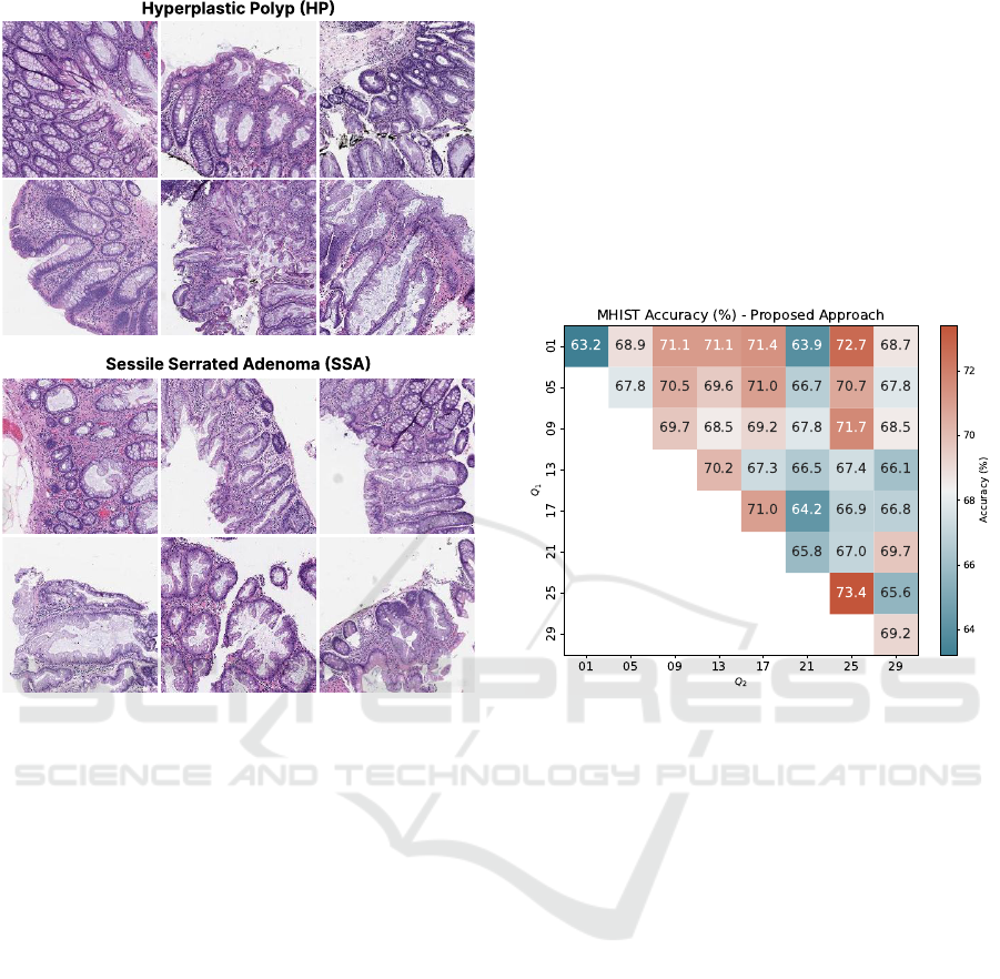
Figure 6: Samples of the MHIST (Wei et al., 2021) dataset.
The first two rows of images corresponds to samples of
Hyperplastic Polyp (HP) a typically benign growths, and
the last two ones correspond to Sessile Serrated Adenoma
(SSA), a precancerous lesion.
Figure 6 presents HP and SSA samples of MHIST.
For the experimental setup, Linear Discriminant
Analysis (LDA) was used as the classifier, utilizing
the pre-defined training and test splits of the MHIST
dataset, consisting of 2,175 and 977 samples, respec-
tively. Furthermore, we used four metrics for evalu-
ation: accuracy, precision, recall, and F-score, due to
their importance in medical applications.
In the experimentation, we evaluated the behav-
ior of our proposed texture descriptor,
⃗
Θ(Q) and
⃗
Ω(Q
1
,Q
2
), by analyzing all possible parameter com-
binations, as outlined in Section 3.2. Figure 7
presents a heatmap of the achieved accuracies. The
main diagonal contains the results for the descrip-
tor
⃗
Θ(Q), since Q
1
= Q
2
, while the off-diagonal
entries show the accuracies for the representation
⃗
Ω(Q
1
,Q
2
). The heatmap revealed that configurations
involving combinations of higher-dimensional pro-
jections,
⃗
Ω(Q
1
,Q
2
), did not result in high accuracies,
probably due to the large size of their feature vectors.
This is evident in the region of Figure 7 delimited
by Q
1
∈ {13, 17,21} and Q
2
∈ {21, 25,29}, which
shows a bluer area. In contrast, the proposed descrip-
tor
⃗
Θ(Q) which does not combine multiple represen-
tations, and the descriptor
⃗
Ω(Q
1
,Q
2
) when combin-
ing low-dimensional projections achieved the high-
est accuracies, such as
⃗
Θ(25) and
⃗
Ω(01,25), which
achieved accuracies of 73.4% and 72.7%, respec-
tively. Therefore, we selected the simple, compact
texture descriptor
⃗
Θ(25) which achieved the highest
accuracy of 73.4%, to be compared with other litera-
ture methods.
Figure 7: Accuracy rates (%) on MHIST dataset for the
proposed approach. The main diagonal corresponds to the
⃗
Θ(Q) descriptor, since Q
1
= Q
2
. The accuracies on the off-
diagonal corresponds to the
⃗
Ω(Q
1
,Q
2
) descriptor.
In Table 6, we presented the comparison of our
proposed approach against other methods in the liter-
ature. The results show that the proposed approach
outperformed all other texture-related methods in re-
lation to accuracy and precision, while ranking sec-
ond for recall and F-score. Compared to another ran-
domized neural network-based approach (SSR), our
method surpassed it by 4.8% in accuracy, correspond-
ing to 47 additional correctly classified images. This
result demonstrates the effectiveness of sliding 3D
color cubes over the images to capture both spatial
(texture) and color (spectral) patterns.
Additionally, we also compared our approach
with various pre-trained deep convolutional neural
networks used as feature extractors. In particular,
our approach achieved higher accuracy and precision
than all compared DCNNs, including VGG11 (0.4%),
ResNet18 (0.4%), ResNet50 (13.8%), DenseNet121
(0.9%), and InceptionResNetV2 (4.5%), where the
values in parentheses denote the accuracy improve-
ment of our approach over each DCNN.
Still, although our method ranks second in recall
VISAPP 2025 - 20th International Conference on Computer Vision Theory and Applications
218

Table 6: Comparison of classification accuracies of differ-
ent literature methods for the very challenging task of clas-
sification of colorectal polyps on the MHIST dataset. Bold
denotes the best result, and underline the second best.
Method Accuracy Precision Recall F-score
GLCM integrative 65.0 61.3 59.2 59.2
Fourier integrative 65.5 62.1 60.5 60.8
Fractal integrative 65.7 62.5 61.3 61.6
LBP integrative 60.1 56.7 56.5 56.6
LPQ integrative 63.1 59.6 58.9 59.0
LCP integrative 68.4 65.7 62.7 63.0
AHP integrative 65.3 62.0 60.8 61.0
BSIF integrative 63.7 60.8 60.6 60.7
CLBP integrative 54.8 54.0 54.2 53.5
LGONBP (gray-level) 62.7 60.0 60.1 60.1
LETRIST (gray-level) 68.5 65.7 63.6 64.0
SWOBP 67.5 64.5 62.4 62.8
SSR 68.6 66.1 65.7 65.9
VGG11 73.0 70.9 70.3 70.6
ResNet18 73.0 71.0 71.2 71.1
ResNet50 59.6 58.9 59.5 58.5
DenseNet121 72.5 70.5 70.6 70.5
InceptionResNetV2 68.9 66.9 67.3 67.0
Proposed Method
VCTex 73.4 71.4 70.6 70.9
and F-score, with ResNet18 achieving the highest val-
ues, improving by 0.6% in recall and 0.2% in F-score,
it is noteworthy that our approach produced competi-
tive results compared to these DCNNs pre-trained on
millions of images, highlighting the robustness of our
simple, fast and low computational cost approach, in
comparison to these larger and expensive DCNNs ar-
chitectures.
Finally, the results demonstrate that our method
outperformed all compared texture methods in accu-
racy, including pre-trained deep convolutional neural
networks used as feature extractors. This result high-
lights the effectiveness of our approach in the very
challenging and important task of classifying colorec-
tal polyps. These findings suggest that our method
could be further explored to other histological image
problems, offering a simple and cost-effective solu-
tion.
4 CONCLUSIONS
In this paper, we proposed a new color-texture rep-
resentation based on randomized autoencoder that si-
multaneously encodes texture and color information
using volumetric (3D) color cubes. For each image,
a 3D color cube slides over the image, capturing both
texture and color (spectral) patterns. These patterns
are then encoded by the randomized autoencoder, and
we use as color-texture representation the flattened
weights of the decoder’s learned weights. The effec-
tiveness of our approach is evidenced by the results
on color-texture datasets, where our method outper-
formed several methods from the literature, including
deep convolutional neural networks.
Moreover, we show the applicability and robust-
ness of the proposed approach in the challenging
and important task of colorectal polyp classifica-
tion, aiding the identification of colorectal cancer us-
ing only texture-related information. Therefore, this
study shows the effectiveness of random encoding
color-texture information using volumetric (3D) color
cubes, culminating in a simple, fast, and efficient ap-
proach. As future work, this method may be adapted
to hyperspectral images, dynamic textures, or alterna-
tive strategies for encoding color cube information.
ACKNOWLEDGEMENTS
R. T. Fares acknowledges support from FAPESP
(grant #2024/01744-8), L. C. Ribas acknowledges
support from FAPESP (grants #2023/04583-2 and
2018/22214-6). This study was financed in part by
the Coordenac¸
˜
ao de Aperfeic¸oamento de Pessoal de
N
´
ıvel Superior - Brasil (CAPES).
REFERENCES
Abdelmounaime, S. and Dong-Chen, H. (2013). New
brodatz-based image databases for grayscale color and
multiband texture analysis. International Scholarly
Research Notices, 2013.
Backes, A. R., Casanova, D., and Bruno, O. M. (2009).
Plant leaf identification based on volumetric fractal
dimension. International Journal of Pattern Recog-
nition and Artificial Intelligence, 23(06):1145–1160.
Backes, A. R., Casanova, D., and Bruno, O. M. (2012).
Color texture analysis based on fractal descriptors.
Pattern Recognition, 45(5):1984–1992.
Backes, A. R., Casanova, D., and Bruno, O. M. (2013). Tex-
ture analysis and classification: A complex network-
based approach. Information Sciences, 219:168–180.
Calvetti, D., Morigi, S., Reichel, L., and Sgallari, F. (2000).
Tikhonov regularization and the l-curve for large dis-
crete ill-posed problems. Journal of Computational
and Applied Mathematics, 123(1):423–446.
Choe, A. R., Song, E. M., Seo, H., Kim, H., Kim, G.,
Kim, S., Byeon, J. R., Park, Y., Tae, C. H., Shim,
K.-N., et al. (2024). Different modifiable risk fac-
tors for the development of non-advanced adenoma,
advanced adenomatous lesion, and sessile serrated le-
sions, on screening colonoscopy. Scientific Reports,
14(1):16865.
Cover, T. M. (1965). Geometrical and statistical properties
of systems of linear inequalities with applications in
pattern recognition. IEEE Transactions on Electronic
Computers, EC-14(3):326–334.
Volumetric Color-Texture Representation for Colorectal Polyp Classification in Histopathology Images
219

Deng, J., Dong, W., Socher, R., Li, L.-J., Li, K., and Fei-
Fei, L. (2009). Imagenet: A large-scale hierarchical
image database. In 2009 IEEE conference on com-
puter vision and pattern recognition, pages 248–255.
Ieee.
Fares, R. T. and Ribas, L. C. (2024). Randomized
autoencoder-based representation for dynamic texture
recognition. In 2024 31st International Conference
on Systems, Signals and Image Processing (IWSSIP),
pages 1–7. IEEE.
Fares, R. T., Vicentim, A. C. M., Scabini, L., Zielinski,
K. M., Jennane, R., Bruno, O. M., and Ribas, L. C.
(2024). Randomized encoding ensemble: A new ap-
proach for texture representation. In 2024 31st Inter-
national Conference on Systems, Signals and Image
Processing (IWSSIP), pages 1–8. IEEE.
Guo, Y., Zhao, G., and Pietik
¨
ainen, M. (2011). Texture clas-
sification using a linear configuration model based de-
scriptor. In BMVC, pages 1–10. Citeseer.
Guo, Z., Zhang, L., and Zhang, D. (2010). A completed
modeling of local binary pattern operator for texture
classification. IEEE Transactions on Image Process-
ing, 19(6):1657–1663.
Haralick, R. M. (1979). Statistical and structural approaches
to texture. Proceedings of the IEEE, 67(5):786–804.
He, K., Zhang, X., Ren, S., and Sun, J. (2016). Deep resid-
ual learning for image recognition. In Proceedings of
the IEEE conference on computer vision and pattern
recognition, pages 770–778.
Hu, S., Li, J., Fan, H., Lan, S., and Pan, Z. (2024).
Scale and pattern adaptive local binary pattern for tex-
ture classification. Expert Systems with Applications,
240:122403.
Huang, G., Liu, Z., Van Der Maaten, L., and Weinberger,
K. Q. (2017). Densely connected convolutional net-
works. In Proceedings of the IEEE conference on
computer vision and pattern recognition, pages 4700–
4708.
Huang, G.-B., Zhu, Q.-Y., and Siew, C.-K. (2006). Extreme
learning machine: Theory and applications. Neuro-
computing, 70(1):489–501.
Kannala, J. and Rahtu, E. (2012). Bsif: Binarized statistical
image features. In Pattern Recognition (ICPR), 2012
21st International Conference on, pages 1363–1366.
IEEE.
Krizhevsky, A., Sutskever, I., and Hinton, G. E. (2012). Im-
ageNet Classification with Deep Convolutional Neu-
ral Networks. Advances In Neural Information Pro-
cessing Systems, pages 1–9.
Li, L., Yao, Z., Gao, S., Han, H., and Xia, Z. (2024). Face
anti-spoofing via jointly modeling local texture and
constructed depth. Engineering Applications of Ar-
tificial Intelligence, 133:108345.
Liu, G.-H. and Yang, J.-Y. (2023). Exploiting deep textures
for image retrieval. International Journal of Machine
Learning and Cybernetics, 14(2):483–494.
Marin
´
o, G. C., Petrini, A., Malchiodi, D., and Frasca, M.
(2023). Deep neural networks compression: A com-
parative survey and choice recommendations. Neuro-
computing, 520:152–170.
Moore, E. H. (1920). On the reciprocal of the general al-
gebraic matrix. Bulletin of American Mathematical
Society, pages 394–395.
Ojala, T., M
¨
aenp
¨
a
¨
a, T., Pietik
¨
ainen, M., Viertola, J.,
Kyll
¨
onen, J., and Huovinen, S. (2002a). Outex - new
framework for empirical evaluation of texture analy-
sis algorithms. Object recognition supported by user
interaction for service robots, 1:701–706 vol.1.
Ojala, T., Pietikainen, M., and Maenpaa, T. (2002b). Mul-
tiresolution gray-scale and rotation invariant texture
classification with local binary patterns. IEEE Trans-
actions on pattern analysis and machine intelligence,
24(7):971–987.
Pao, Y.-H., Park, G.-H., and Sobajic, D. J. (1994). Learning
and generalization characteristics of the random vec-
tor functional-link net. Neurocomputing, 6(2):163–
180.
Pao, Y.-H. and Takefuji, Y. (1992). Functional-link net com-
puting: theory, system architecture, and functionali-
ties. Computer, 25(5):76–79.
Paszke, A., Gross, S., Massa, F., Lerer, A., Bradbury, J.,
Chanan, G., Killeen, T., Lin, Z., Gimelshein, N.,
Antiga, L., Desmaison, A., Kopf, A., Yang, E., De-
Vito, Z., Raison, M., Tejani, A., Chilamkurthy, S.,
Steiner, B., Fang, L., Bai, J., and Chintala, S. (2019).
PyTorch: An Imperative Style, High-Performance
Deep Learning Library. In Advances in Neural In-
formation Processing Systems 32, pages 8024–8035.
Curran Associates, Inc.
Penrose, R. (1955). A generalized inverse for matrices.
Mathematical Proceedings of the Cambridge Philo-
sophical Society, 51(3):406–413.
Rangaiah, P. K., Augustine, R., et al. (2025). Improving
burn diagnosis in medical image retrieval from graft-
ing burn samples using b-coefficients and the clahe al-
gorithm. Biomedical Signal Processing and Control,
99:106814.
Ribas, L. C., Scabini, L. F., Condori, R. H., and Bruno,
O. M. (2024a). Color-texture classification based
on spatio-spectral complex network representations.
Physica A: Statistical Mechanics and its Applications,
page 129518.
Ribas, L. C., Scabini, L. F., de Mesquita S
´
a Junior, J. J., and
Bruno, O. M. (2024b). Local complex features learned
by randomized neural networks for texture analysis.
Pattern Analysis and Applications, 27(1):1–12.
S
´
a Junior, J. J. d. M. and Backes, A. R. (2016). Elm based
signature for texture classification. Pattern Recogni-
tion, 51:395–401.
S
´
a Junior, J. J. d. M., Backes, A. R., and Bruno, O. M.
(2019). Randomized neural network based signature
for color texture classification. Multidimensional Sys-
tems and Signal Processing, 30(3):1171–1186.
Scabini, L. F., Condori, R. H., Gonc¸alves, W. N., and Bruno,
O. M. (2019). Multilayer complex network descrip-
tors for color–texture characterization. Information
Sciences, 491:30–47.
Schmidt, W., Kraaijveld, M., and Duin, R. (1992). Feed-
forward neural networks with random weights. In
Proceedings., 11th IAPR International Conference on
VISAPP 2025 - 20th International Conference on Computer Vision Theory and Applications
220

Pattern Recognition. Vol.II. Conference B: Pattern
Recognition Methodology and Systems, pages 1–4.
Simonyan, K. and Zisserman, A. (2014). Very deep con-
volutional networks for large-scale image recognition.
CoRR, abs/1409.1556.
Song, T., Feng, J., Luo, L., Gao, C., and Li, H. (2020a).
Robust texture description using local grouped order
pattern and non-local binary pattern. IEEE Transac-
tions on Circuits and Systems for Video Technology,
31(1):189–202.
Song, T., Feng, J., Wang, S., and Xie, Y. (2020b). Spa-
tially weighted order binary pattern for color tex-
ture classification. Expert Systems with Applications,
147:113167.
Song, T., Li, H., Meng, F., Wu, Q., and Cai, J. (2017).
Letrist: Locally encoded transform feature histogram
for rotation-invariant texture classification. IEEE
Transactions on circuits and systems for video tech-
nology, 28(7):1565–1579.
Su, Y., Yan, P., Lin, J., Wen, C., and Fan, Y. (2024). Few-
shot defect recognition for the multi-domain industry
via attention embedding and fine-grained feature en-
hancement. Knowledge-Based Systems, 284:111265.
Szegedy, C., Ioffe, S., Vanhoucke, V., and Alemi, A. A.
(2017). Inception-v4, inception-resnet and the impact
of residual connections on learning. In Thirty-First
AAAI Conference on Artificial Intelligence.
Tikhonov, A. N. (1963). On the solution of ill-posed prob-
lems and the method of regularization. Dokl. Akad.
Nauk USSR, 151(3):501–504.
Wang, Y., Huang, G., Song, S., Pan, X., Xia, Y., and Wu,
C. (2021). Regularizing deep networks with seman-
tic data augmentation. IEEE Transactions on Pattern
Analysis and Machine Intelligence, 44(7):3733–3748.
Wei, J., Suriawinata, A., Ren, B., Liu, X., Lisovsky, M.,
Vaickus, L., Brown, C., Baker, M., Tomita, N., Torre-
sani, L., et al. (2021). A petri dish for histopathology
image analysis. In International Conference on Artifi-
cial Intelligence in Medicine, pages 11–24. Springer.
Weszka, J. S., Dyer, C. R., and Rosenfeld, A. (1976). A
comparative study of texture measures for terrain clas-
sification. IEEE transactions on Systems, Man, and
Cybernetics, (4):269–285.
Zhu, Z., You, X., Chen, C. P., Tao, D., Ou, W., Jiang,
X., and Zou, J. (2015). An adaptive hybrid pattern
for noise-robust texture analysis. Pattern Recognition,
48(8):2592–2608.
Volumetric Color-Texture Representation for Colorectal Polyp Classification in Histopathology Images
221