Assessing the Influence of scRNA-Seq Data Normalization on

Dimensionality Reduction Outcomes

Marcel Ochocki

, Michal Marczyk

1,2 b

and Joanna Zyla

Department of Data Science and Engineering, Silesian University of Technology, Akademicka 16, Gliwice, Poland

Breast Medical Oncology, Yale Cancer Center, Yale School of Medicine, New Haven, CT, U.S.A.

Keywords: Unsupervised Learning, Data Normalization, Dimensionality Reduction, Single-Cell Sequencing.

Abstract: Through the decades, improvements in high-throughput molecular biology techniques have brought to the

level of sequencing transcripts from single cells (scRNA-Seq) instead of bulk material. Implementing these

new techniques requires innovative analytical methods and knowledge about their performance. Data

normalization is a crucial step in the bioinformatical pipeline applied in scRNA-Seq analysis. We evaluated

the impact of six commonly used normalization methods on two dimensionality reduction methods, namely

tSNE and UMAP, using three real scRNA-Seq datasets. We tested dispersion and clustering efficiency using

three clustering algorithms after dimensionality reduction. Our results demonstrated that simple normalization

methods, such as log2 or Freeman-Tukey, as well as scran normalization consistently outperformed other

scRNA-seq-dedicated techniques, yielding superior dimensionality reduction and clustering efficiency for

small and medium-sized datasets. Regardless of no statistically significant enhancement in results for any

dimensionality reduction methods or clustering techniques, the Louvain clustering method consistently

demonstrated lower performance results. We conclude, that the choice of normalization technique should be

carefully tailored to the dataset’s size and characteristics since it may affect the final within-pipeline

processing results.

1 INTRODUCTION

Recent advances in RNA sequencing technologies

have increased the sensitivity and specificity of

transcriptome analysis. The latest solutions allow for

precise analysis of transcript heterogeneity and reveal

novel subpopulations and cell types on an individual

cell level (single-cell RNA sequencing; scRNA-Seq).

Yet, the introduction of scRNA-Seq brought many

challenges to bioinformatical analysis (Hwang et al.,

2018). One of the first steps in scRNA-Seq analysis

is data normalization which reduces technical noise

and existing biases. Moreover, normalization results

in comparable gene counts within and between cells

that allow for more precise downstream analysis.

Throughout the development of scRNA-seq, a variety

of normalization methods have been employed,

including adaptations of bulk sequencing techniques

(Hafemeister and Satija, 2019) as well as novel

https://orcid.org/0009-0001-0814-3431

https://orcid.org/0000-0003-2508-5736

https://orcid.org/0000-0002-2895-7969

approaches specifically designed for scRNA-Seq

studies. Yet, the first one can overcorrect for scaling

factor sizes (Vallejos et al., 2017). Recently, many

normalization methods were introduced and several

studies tested their efficiency and impact on further

analysis (Cole et al., 2019, Vieth et al., 2019). In

(Lytal et al., 2020) authors assessed using empirical

visualization, impact on classification, and

computational time. In (Brown et al., 2021) authors

introduced a new normalization method (Dino) with

comparison to other solutions and tested their

influence on differential expression analysis based on

a relationship between average TPR and average FPR

for a Wilcoxon rank-sum test, as well as on clustering.

Finally, one of the biggest studies (Ahlmann-Eltze

and Huber, 2023) tested methods for consistency,

simulation, and downsampling.

In the presented manuscript, we concentrated on

the impact of the normalization step on dimensiona-

504

Ochocki, M., Marczyk, M. and Zyla, J.

Assessing the Inﬂuence of scRNA-Seq Data Normalization on Dimensionality Reduction Outcomes.

DOI: 10.5220/0013318700003911

Paper published under CC license (CC BY-NC-ND 4.0)

In Proceedings of the 18th International Joint Conference on Biomedical Engineering Systems and Technologies (BIOSTEC 2025) - Volume 1, pages 504-515

ISBN: 978-989-758-731-3; ISSN: 2184-4305

lity reduction outcomes and their clustering ability.

The dimensionality reduction by tSNE or UMAP is

one of the most common ways to present scRNA-Seq

data studies (Cakir et al., 2020). Moreover, it is one

of the most important steps to visualize the

heterogeneity of the analyzed dataset. Thus, joint

solutions were also introduced to compare different

datasets (j-tSNE and j-UMAP) (Do and Canzar,

2021). Yet, to our best knowledge, the impact of

normalization to reductions given by tSNE and

UMAP was not tackled before in non-empirical way.

To reach the gain of the study we collected three

real scRNA-Seq datasets with known cell labels and

different sample sizes, for which we ran six different

normalization techniques. Next, based on normalized

data we extracted the tSNE and UMAP 2D

embeddings and measured the effect of normalization

on dispersion in dimensionality reduction. Moreover,

we checked the impact of normalization on clustering

performance based on 2D transformed data by three

different clustering methods.

2 MATERIALS AND METHODS

2.1 scRNA-Seq Datasets

Three scRNA-Seq datasets of diverse sample sizes

and labeled cell types were used to assess the quality

of performed clustering (Table 1). The first dataset,

called Liver, including immunological cells, was

extracted from liver tissue (Wang et al., 2021) and is

available under access number E-MTAB-10553. The

dataset includes 15,650 labeled cells divided into 13

groups. The second dataset, PBMC, provides

information from peripheral blood mononuclear cells

(Ding et al., 2020). Only experiment 1A performed

on Chromium v2 10x platform, where 3,222 cells

were grouped into 9 cell types, was used here. The

data are available at the single-cell portal of Broad

Institute (https://singlecell.broadinstitute.org). The

smallest dataset includes cells derived from different

tissues of breast cancer (BC) subtypes (HER+,

Luminal A, Luminal B, and Tripple Negative Breast

Cancer) as well as normal ones (Chung et al., 2017).

Due to the presence of samples from healthy tissue,

this dataset was investigated in two ways: (i) with all

possible groups i.e. 5 (BC_sub), and (ii) healthy vs

cancer tissue cells (BC_dis). The dataset is publicly

available under access number E-GEOD-75367.

For every dataset, three pre-processing steps were

performed: (i) transcripts with only zero counts across

all cells and with low variance of normalized

expression were filtered out using GaMRed (Marczyk

et al., 2018); (ii) transcripts without annotation were

removed; (iii) for the transcripts with duplicated

Ensembl ID the one with higher variance were kept.

Table 1: Summary of used scRNA-Seq datasets.

Dataset # of

samples

# of

features

# of cell

types /

classes

Liver 15000 15,650 13

PBMC 3,222 15,817 9

Breast Cancer

(BC_sub)

244 16,639 5

Breast Cancer

(BC_dis)

244 16,639 2

2.2 Data Normalization Methods

Several normalization techniques widely used in

scRNA-seq data analysis were tested (Table 2). Both,

primary methods like the log2 transformation and the

Freeman-Tukey square root (FT) transformation, as

well as several novel normalization techniques

specifically suited for scRNA-seq data, were

included. Before basic transformations, data were

scaled by the median counts across all cells to

mitigate the sequencing-depth normalization and

stabilize the variance across the different gene

expression levels.

2.2.1 Simple Transformations

Logarithmic normalization, particularly the log2

transformation, is a popular choice for reducing

distribution skewness and is typically used in

standard RNA-seq preprocessing pipelines before

downstream feature selection (Luecken et al., 2019,

Lytal et al., 2020, Cuevas-Diaz et al., 2024).

Importantly, before applying the log2 transformation,

a small ‘pseudocount’ of one was added to all gene

counts to account for both technical and cell-specific

absences of transcript counts. This step is a well-

established standard in such a pipeline (Lytal et al.,

2020).

Square root transformation, though less common

than logarithmic one, is another effective

normalization technique in scRNA-seq data

processing (Lause et al., 2021, Booeshaghi et al.,

2022). The choice of square root transformation,

especially the FT transformation, is often vastly

justified by the characteristics of scRNA-seq data,

which are frequently modeled using a Poisson

distribution (Brown et al., 2021, Lause et al., 2021,

Choudhary and Satija, 2022).

Assessing the Inﬂuence of scRNA-Seq Data Normalization on Dimensionality Reduction Outcomes

505

2.2.2 Scran – Normalization via

Deconvolution Across Pooled Cells

The Scran normalization method (Lun et al., 2016)

aims to enhance overall normalization efficiency

through a deconvolution process. The core objective

of this approach is to estimate the adjusted cell

transcript count based on cell-specific parameters,

which describe the cell bias and its corresponding

adjustment factor, respectively. However, to obtain

unbiased estimates of true expressions, several

assumptions and computations must be taken into

account. First of all, cell pools are created by

grouping cells with similar library sizes. This is a

pivotal step in Scran normalization, that helps to

reduce variability arising from technical differences,

e.g. sequencing depth. Next, the pool-based size

factor can be determined as the ratio of the sum of

transcript counts within the k-th pool, and

the mean of

gene counts across the entire cell population. The

estimates of the factor within all cell pools are then

calculated as the median across genes, based on the

assumption that the majority of genes are non-

differentially expressed. Based on that, we can

construct a system of linear equations to estimate the

cell-specific biases, that finally can be solved with a

standard least-squares method.

2.2.3 SCnorm – Normalization Using

Quantile Regression with Gene

Grouping

The SCnorm approach (Bacher et al., 2017) models

the relationship between gene log-transformed

expression counts and the corresponding cells' log-

transformed sequencing depth (hereafter, the ‘log-

transformed’ participle will be omitted for

simplicity). The genes are initially grouped into K

pools (by default at the first step K=1) to preserve cell

variability. For each of these K groups, the

relationship between gene expression counts and

sequencing depth is modeled using median quantile

regression for each gene and cell. Additionally,

quantile regression is employed to estimate a similar

relationship for the overall expression of all genes.

SCnorm assumes that the median may not always be

the best estimate for the entire set of genes, thus it

considers multiple quantiles, as well as several

degrees of polynomial, to improve accuracy. The

authors propose that the optimal quantiles and

degrees minimize the difference between the count-

depth relationship value across predicted expressions,

estimated via median regression using a first-degree

polynomial, and the mode of such a relationship for

un-normalized counts. The scale factor for each cell

is computed based on the estimated quantiles for each

group. Specifically, for each gene group, the scale

factor for a cell is defined as the ratio between the

gene expression values at a selected quantile and the

corresponding predicted values from the regression

model. Moreover, to adjust the number of K, a

specific condition is defined; the modes of the slopes

within equal-sized gene groups must be less than 0.1.

If at least one of them is greater, the initial number of

K = 1 is increased by one, and the genes are pooled

across groups with the k-medoids algorithm.

However, the authors suggested considering pre-

defined conditions under which the normalization

procedure may proceed before being applied to the

entire dataset. To maintain the unsupervised nature of

the pipeline, we decided to pre-aggregate cells into

separate groups using hierarchical clustering, as

described in the supplementary materials provided in

the Bioconductor guides.

2.2.4 Dino – Normalization by

Distributional Resampling

Dino (Brown et al., 2021) is an approach that aims to

reconstruct transcript expression distributions that are

independent of the cell’s library size. Those

distributions are Poisson means modeled as Gamma

mixtures. In this study, the number of Gamma

components is set to 100, as a default value proposed

in the original paper. The normalized values of

transcript expression can be sampled from the

posterior distribution with an additional

concentration parameter, that reduces the variability

and centers the normalized values (set to 15, as

originally proposed by the authors).

2.2.5 SCtransform – Normalization with

Variance Stabilization Using

Regularized Negative Binomial

Distribution

The SCtransform normalization method (Hafemeister

and Satija, 2019) utilizes generalized linear models

with regularized Negative Binomial distributions to

model un-normalized transcript counts. Each model

is fitted separately for individual genes, based on the

assumption that uniform scaling factors across all

genes result in inefficient normalization, particularly

for high and medium-high abundance transcripts. To

prevent overfitting, the model parameters are

regularized by pooling information across genes with

similar average expression levels. To learn robust and

smoothed parameter estimates, the Kernel regression

BIOINFORMATICS 2025 - 16th International Conference on Bioinformatics Models, Methods and Algorithms

506

is applied. Finally, the true gene counts are calculated

as Pearson residuals. An improved version of the

method was chosen (Choudhary and Satija, 2022)

which excludes low-expressed genes from

regularization.

Table 2: Summary of applied scRNA-Seq data

normalization along with R package used.

Method Source Ver.

log2 - -

Freeman-

Tuke

- -

SCtransform

https://cran.r-

project.org/web/packages/Se

urat/index.html

5.1.0

scran

https://bioconductor.org/pac

kages/devel/bioc/vignettes/s

cran/inst/doc/scran.html

1.32.0

Dino

https://www.bioconductor.or

g/packages/release/bioc/html

/Dino.html

1.10.0

SCnorm

https://github.com/rhondaba

cher/SCnor

1.26.0

2.2.6 Normalized Transcript Post-

Processing

After applying all normalization methods, only the

top 20% of genes with the highest between-cells

normalized transcript variance was left to potentially

filter out non-differentially expressed ones. Next,

principal component analysis was performed and the

first 50 principal components were taken for further

analysis to reduce background noise of data.

2.3 Unsupervised Learning

For normalized and filtered data the following

unsupervised learning techniques were applied: (i)

two dimensionality reduction methods, and (ii) three

clustering methods.

2.3.1 Dimensionality Reduction

The first method was t-distributed stochastic neighbor

embedding (tSNE) (Van der Maaten and Hinton,

2008). At first, similarities between data points are

estimated (Euclidean distance here) and then

transformed into probabilities using Gaussian kernel

(high-dimensional space). Next, the low-dimensional

space is randomly generated for which each data

point has an assigned position. Similarly, the pairwise

similarities between data points are computed but

with the usage of t-distribution. The goal of tSNE is

to minimize the divergence between the pairwise

similarities in the high-dimensional space and

corresponding similarities in the low-dimensional

space. This procedure allows to preserve local

relationships and clusters within the data.

The second applied procedure was Uniform

Manifold Approximation and Projection (UMAP)

(McInnes, 2018). At first, pairwise similarities

between data points are calculated using specified

metrics (Euclidean metric here). Next, local

neighborhood structure is created based on pairwise

similarities. The optimization process between, a

random low-dimensional embedding and high-

dimensional structure is done by stochastic gradient

descent which minimizes the discrepancy between

the pairwise similarities of spaces. Moreover, the

UMAP procedure allows to preserve not only the

local relationships like tSNE but also the global ones

by constructing graph representation based on the

low-dimensional embedding (updated in iterations)

2.3.2 Clustering Algorithms

To evaluate the influence of normalization on

clustering outcomes, several common methods were

chosen. For each method, the Euclidean distance

metric was used. The optimal number of clusters was

determined by maximizing the Silhouette Index (SI)

value (Rousseeuw, 1987), calculated as the mean of

the Silhouette values computed for the entire dataset.

The first method used in this paper was k-means

(MacQueen, 1967). The main idea behind k-means is

to group observations into k pre-defined clusters,

minimizing the overall distance of each point to the

centroid of its respective cluster. When the

observations are assigned to each cluster, the

centroids are recalculated iteratively, until the loss

function reaches a plateau. Since the algorithm begins

with random initial conditions (where the preliminary

centroids are chosen from the data points), it may

produce non-deterministic outcomes. Therefore, to

find the optimal solution, it is recommended to run

the algorithm multiple times for the same pre-defined

value of k.

The second approach was hierarchical clustering

(h-clust). Specifically, agglomerative, complete-

linkage h-clust was employed, where clusters with the

smallest between-cluster distance are iteratively

combined into larger groups. This process continues

until all objects are grouped into a single cluster. In

the complete-linkage form, the between-cluster

distance is measured between the two furthest points

of each cluster (Hubert, 1974).

As the third method, the Louvain community

detection approach was used (Blondel et al., 2008).

Assessing the Inﬂuence of scRNA-Seq Data Normalization on Dimensionality Reduction Outcomes

507

Here, each cell is considered as a node and initially

assigned to its cluster. The algorithm iterates through

each node in the network, calculating the change in

modularity that would result from moving the node to

each of its neighboring clusters. If the modularity

increases, the node is merged with the cluster. This

step is repeated as long, as the increase in modularity

is no further observed. Then, the clusters are

aggregated, creating a set of new meta-communities,

and forming the nodes of a new network. The weights

of links between these meta-communities are

calculated as the sum of the weights of links between

the nodes in the corresponding original clusters. The

process is sequentially repeated, until the modularity

reaches its maximum and no further changes in

community structure occur. Before clustering, a

graph structure using the k-nearest neighbors

algorithm was constructed. To find the optimal

number of clusters, k was changed within the range 5-

100 with a step equal to 5, and the resolution

parameter from 0.4 to 2, with a step equal to 0.1.

2.4 Performance Metrics Used in

Evaluation

The silhouette index was used to estimate the effect

of normalization on dispersion after dimensionality

reduction. The index was also calculated for original

labels for comparison. The second evaluation relied

on clustering performance itself. For that, the

Adjusted Rand Index (ARI, Rand, 1971), Dice-

Sørensen coefficient (Dice, 1945; Sørensen, 1948),

and Mutual Information (Shannon, 1948) measures

were calculated.

Kruskal-Wallis test (Kruskal and Wallis, 1952)

was applied with Conover post-hoc (Conover and

Iman, 1979) to assess the difference in clustering

performance between normalization techniques. The

significance level was set to α=0.05. Additionally, the

effect size was measured using Cohen’s d modified

Conover’s d coefficient to support our inference.

During the final analysis, clustering and

dimensionality reduction methods were compared for

the same measures and statistical tests as in the

clustering performance evaluation. However, to test

differences between tSNE and UMAP the Wilcoxon

test was used (Wilcoxon, 1945).

All testing was conducted on the same PC with the

following parameters: Intel Core i5-10500 CPU @

3.10 GHz, and 64 GB of RAM. For all calculations,

computational time was collected and evaluated

alongside other performance metrics to ensure

comprehensive analysis. Furthermore, if parallel

computation was enabled within the implemented

functions, the number of cores to utilize was set to the

maximum available.

3 RESULTS

3.1 Effect of Normalization on Data

Dispersion in Reduced Space

For the BC_dis dataset reduced using tSNE, the

Kruskal-Wallis test indicated a significant difference

between methods (Figure 1A). Post-hoc Conover

tests revealed statistically significant differences

compared to non-normalized data for log2

normalization (p-value < 5.5e-6) and scran

normalization (p-value < 1.8e-9). Interestingly, FT

transformation achieved significance only before the

Bonferroni correction (uncorrected p-value = 0.03;

corrected p-value = 0.67). Conover's d effect sizes

suggest moderate effects for log2 (d = 0.47) and scran

(d = 0.59), while FT normalization exhibited a small

effect (d = 0.21) (Figure 2). In contrast, when using

UMAP for dimensionality reduction, the Kruskal-

Wallis test yielded insignificant results (Figure 1A)

marking a drastic change in findings between

reduction methods.

For the BC_sub dataset reduced using tSNE, the

Kruskal-Wallis test revealed highly significant

differences (p-value < 2.2e-16, Figure 1B). Pairwise

Conover tests confirmed significant differences for

FT (p-value < 1.3e-29), log2 (p-value < 2.8e-47), and

scran (p-value < 1.2e-50) normalizations, with large

effect sizes (d = 1.07, d = 1.37, and d = 1.42,

respectively, Fig 2). The other normalization

techniques yielded relatively small effect sizes. When

UMAP was used for dimensionality reduction, the

Kruskal-Wallis test results remained significant, but

the Conover pairwise comparisons revealed even

greater significance for FT, log2, and scran

normalizations, with corresponding effect sizes of d =

1.25, d = 1.48, and d = 1.78, respectively (Figure 2).

For the PBMC dataset, the Kruskal-Wallis test

produced significant results regardless of the

dimensionality reduction method (Figure 1C).

Pairwise multiple comparisons revealed significant

outcomes for all normalization techniques except

SCnorm. However, large effect sizes were observed

only for FT, log2, and scran normalizations. Under

tSNE, the effect sizes were d = 0.98, d = 1.04, and d

= 1.14, respectively, while UMAP yielded slightly

different effect sizes of d = 0.84, d = 1.14, and d =

1.09, respectively (Figure 2).

BIOINFORMATICS 2025 - 16th International Conference on Bioinformatics Models, Methods and Algorithms

508

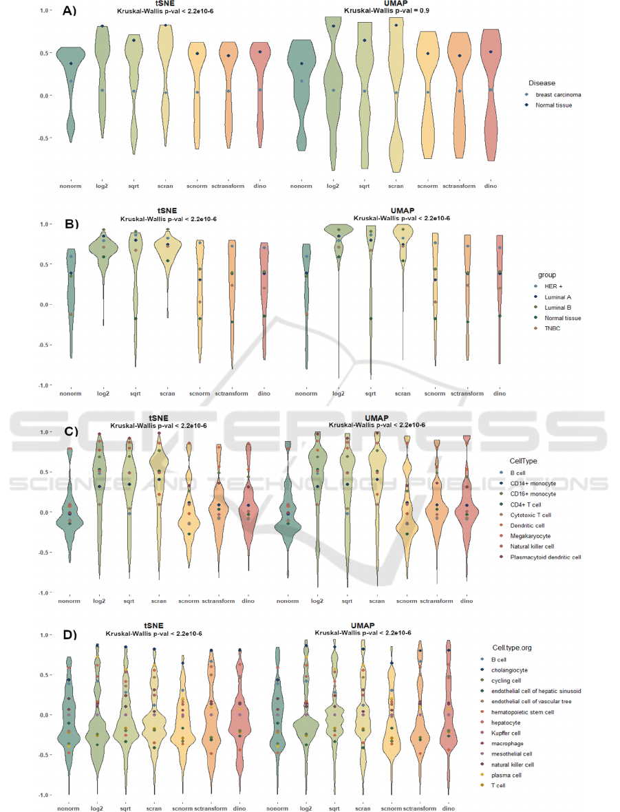
Figure 1: The violin plots illustrate the distribution of SI values after dimensionality reduction with t-SNE (left) and UMAP

(right) across all normalizations. Each point represents the mean SI values calculated across cell types. The panels show

results for A) PBMC, B) breast cancer disease, C) breast cancer subtypes, and D) liver datasets.

Assessing the Inﬂuence of scRNA-Seq Data Normalization on Dimensionality Reduction Outcomes

509

Figure 2: Results of multiple pairwise comparison. The color indicates p-value ranges after Bonferroni's correction, while the

values inside the boxes indicate the Conover’s d effect size.

In contrast to the other datasets, the Liver dataset

showed variation in outcomes depending on the

dimensionality reduction method used, despite the

Kruskal-Wallis test remaining significant overall

(Figure 1D). For tSNE, neither scran nor FT methods

reached significance, with the highest effects

observed for log2 (d = 0.25), SCnorm (d = 0.11), and

SCtransform (d = 0.09). When UMAP was applied,

log2 and scran normalizations failed to achieve

significant results. The greatest, even relatively small

effect sizes, were observed for SCnorm (d = 0.33),

SCtransform (d = 0.22), and FT (d = 0.11) (Figure 2).

These differences underscore the influence of the

dimensionality reduction method on the results.

3.2 Clustering Performance after

Normalization with Different

Methods

In BC_dis, for both ARI and MI, log2 and scran

normalization techniques outperformed all other

methods, particularly when applied in combination

with tSNE. FT transformation demonstrated better

performance than scran in scenarios where UMAP

was utilized. Overall, log2 and scran normalization

enabled the achievement of the best results for k-

means clustering, especially when paired with tSNE

(Figure 3A). For Dice and SI metrics, all techniques

produced relatively similar results, but slight

improvements were observed with Dice when

combined with tSNE, while UMAP yielded

noticeably better outcomes for SI.

For the BC_sub, when combined with tSNE, the

results across various clustering methods consistently

demonstrated the superior performance of both log2

and scran normalizations. In contrast, when paired

with UMAP, FT normalization performed slightly

better than scran. Furthermore, these normalization

techniques enabled k-means clustering to outperform

the other clustering methods (Figure 3B).

In PBMC, according to Dice values, the weakest

outcomes were observed with log2, FT, and scran

normalizations, while the best results were achieved

using tSNE combined with k-means clustering

(Figure 3C). In the case of MI values, and for Louvain

clustering, all normalization methods, except

SCnorm, demonstrated relatively better performance

compared to non-normalized data. In an overall

comparison, log2, FT, and scran normalization

methods outperformed the others. In Louvain

clustering, the choice of dimensionality reduction

method did not significantly impact the results,

except for dino, which showed a marked

improvement when combined with UMAP. It is

BIOINFORMATICS 2025 - 16th International Conference on Bioinformatics Models, Methods and Algorithms

510

worth mentioning that SCransform followed by

UMAP and clustering with either h-clust or k-means

yielded results even worse than non-normalized data.

ARI results consistently highlighted the advantages

of log2, FT, and scran normalization techniques,

particularly when combined with tSNE and k-means

clustering. In contrast to non-normalized data, SI

values showed little to no improvement when reduced

with tSNE across all clustering methods. However,

the scenario drastically changed when UMAP was

used. Here, improvements were observed across all

normalizations, with notable gains seen in k-means

and h-clust, especially with FT, log2, scran, and dino

techniques.

In contrast to the previous datasets, in liver for

tSNE reduction, only SCnorm normalization led to

improved ARI values compared to non-normalized

data - and this improvement was observed exclusively

after applying k-means clustering (Figure 3D). For

UMAP, small improvements were noted with

SCtransform, while the other normalization methods

resulted in performance deterioration. Similar trends

were observed for Dice coefficient values. For MI

values, when tSNE was used, all normalization

methods led to slight improvements. However, log2,

FT, and scran showed marginally better performance

compared to the others. When UMAP was applied,

the results improved across all normalization

methods, with the best outcomes achieved using the

same methods as in tSNE. It was observed that the

performance of SCnorm varied depending on the

dimensionality reduction method and clustering

technique. SCnorm performed worse with tSNE but

showed significantly better performance with UMAP

when followed by h-clust. Similarly, dino

normalization performed substantially better with

tSNE but slightly worse with UMAP when followed

by k-means clustering. The SI values were relatively

poor, similar to those observed with the PBMC

dataset. However, overall performance improved

when the data was reduced using UMAP.

3.3 Unsupervised Method Impact

We observed differences in clustering efficiency

across the same normalization methods with varying

dimensionality reduction methods. Therefore, the

results were compared between these reduction

methods, with particular attention to the clustering

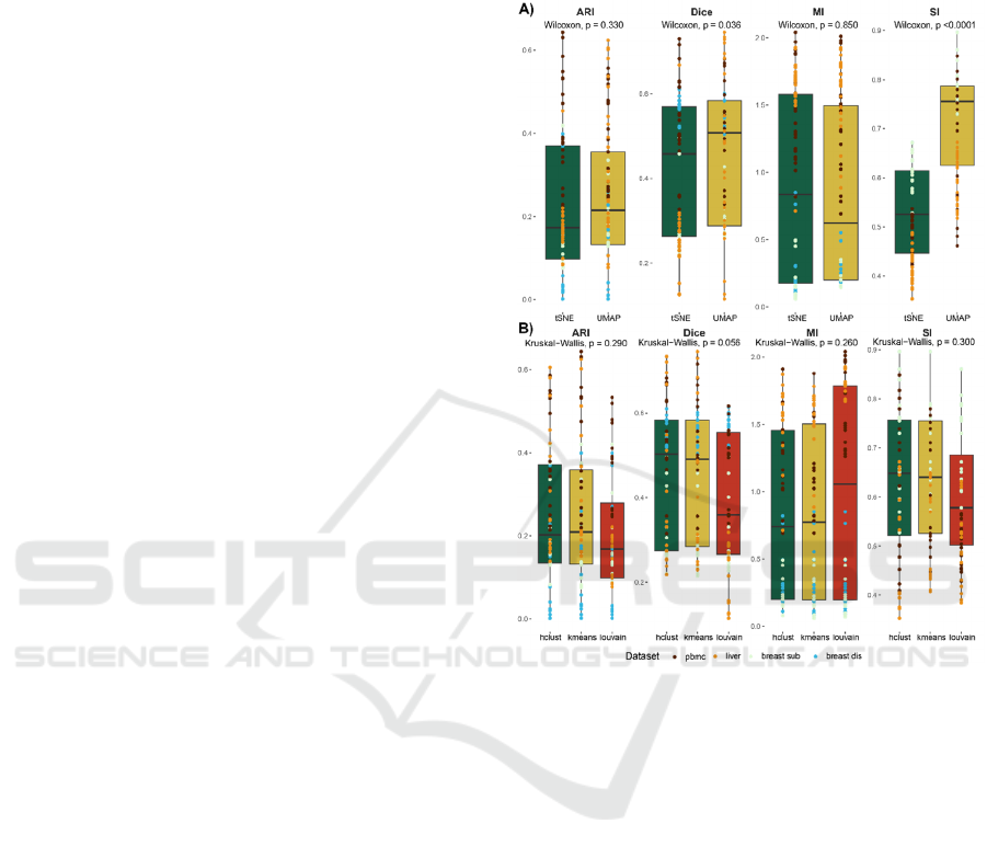
metrics utilized in this study. The results of Wilcoxon

testing (Figure 4A) showed no statistically significant

differences for both ARI and MI metrics. Although,

such differences exist for Dice and SI. Kruskal-Wallis

test did not reveal statistically significant differences

between clustering methods for any of the approaches

used (Figure 4B), though, Louvain performed slightly

worse compared to both k-means and h-clust.

Figure 3: Results evaluated on aggregated datasets. Panel

A) represents a comparison of dimensionality reduction

methods, without distinguishing between clustering

methods. Panel B) represents a comparison of clustering

method without division between dimensionality reduction.

For each comparison, the corresponding Wilcoxon’s test p-

values are indicated.

3.4 Computational Time

Finally, we investigated computational time of tested

normalizations (Table 3) as well as dimensionality

reduction methods (Table 4). As can be observed all

normalizations computational time increase with the

increasing number of samples/cells in experiment. As

expected the simplest mathematical procedures were

the fastest i.e. the log2 and FT normalization. Next

scran and SCtransform can be distinguished. The

worst time performance was observed for

SCnorm. A

similar trend was observed for dimensionality reduction

methods, however, UMAP significantly outperformed

tSNE in terms of computational time.

Assessing the Inﬂuence of scRNA-Seq Data Normalization on Dimensionality Reduction Outcomes

511

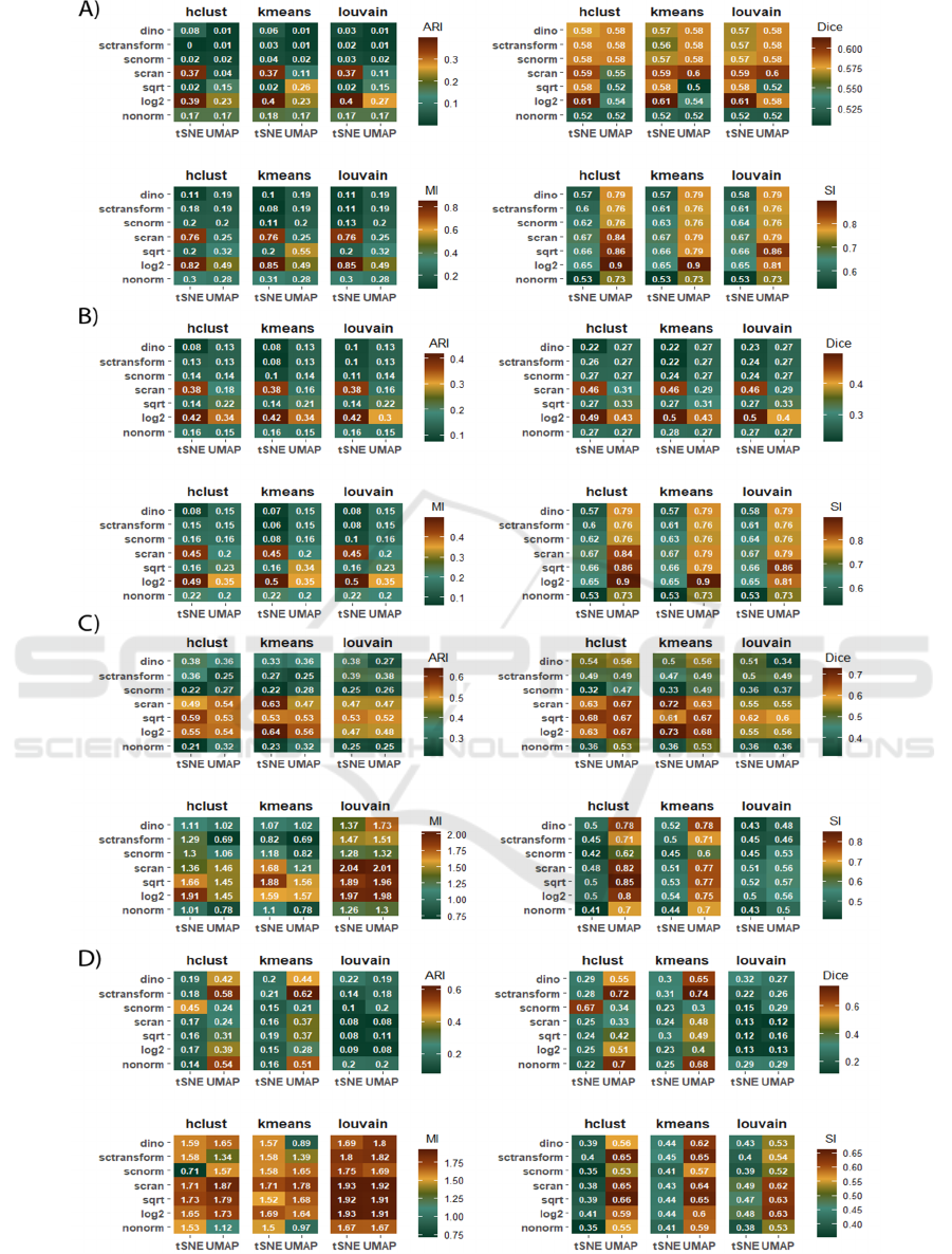
Figure 4: Comparison of clustering efficiency measures calculated with distinction to both normalization and dimensionality

reduction methods. Each subplot presents metric values for ARI, Dice, MI, and SI, arranged from top left to bottom right.

Subsequent subplots show results for A) breast cancer disease, B) breast cancer subtypes, C) PBMC, and D) liver datasets.

BIOINFORMATICS 2025 - 16th International Conference on Bioinformatics Models, Methods and Algorithms

512

Table 3: Computational time of normalization methods (in

seconds).

Dataset Liver PBMC

Breast

Cancer

log2 12.31 2.02 0.25

Freeman-Tukey 6.46 0.58 0.18

SCtransform 117.33 25.55 7.00

scran 93.72 17.55 2.70

Dino 2431.92 459.36 295.98

SCnorm 15850.23 3682.53 7640.03

Table 4: Computational time of dimensionality reduction

methods by average across normalizations (in seconds).

Dataset Liver PBMC Breast Cancer

UMAP 25.06 10.71 1.78

t-SNE 474.84 105.82 0.89

4 DISCUSSION AND

CONCLUSIONS

This study thoroughly examined the impact of

specific data normalization methods on the efficiency

of scRNA-seq data downstream analysis. Our results

indicate that simple normalization methods, such as

log2 and scran consistently enabled obtaining

superior outcomes compared to scRNA-seq domain-

specific techniques, especially for the small and

medium-sized datasets. Moreover, depending on the

dimensionality reduction method leveraged in the

processing, FT normalization sometimes obtains

superior performance compared to scran. However,

as dataset size increases, the performance gap

between simple normalizations and scRNA-seq-

specific techniques diminishes. This observation

suggests that for large and extra-large datasets,

specialized normalization techniques may become

essential to achieve optimal results. On the other

hand, the SCnorm, SCtransform, and dino techniques

appear to be sensitive to specific steps within the

overall pipeline procedure, a trend particularly

noticeable with the larger, Liver dataset. Therefore,

we strongly recommend to be aware when deciding

whether to use simple or domain-specific techniques.

It is worth noting that, in addition to overall

outcomes and performance measures, domain-

specific techniques demand significantly more

computing time. SCnorm normalization, in particular,

is better suited for smaller datasets, as its

computational requirements increase drastically with

larger datasets containing thousands of cells. Similar

conclusions also occur in the literature (Zhang et al.,

2023). Consequently, its inferior performance

compared to other methods, especially for smaller

datasets, is particularly surprising. The observed

dependence was made on few datasets and large scale

research is still needed.

In the overall comparison, it was noticed, that for

a smaller breast cancer dataset, tSNE enabled to

achieve slightly better clustering outcomes than

UMAP, regardless of the level of cell-type

differentiation. On the other hand, UMAP achieved

even statistically significant better results within SI

metric. However, these differences likely arise from

the specific manner in which UMAP performs

dimensionality reduction. Finally, the type of

normalization technique used before reduction may

affect the final level of data dispersion. Yet, presented

research does not include all dimensionality reduction

techniques like variational autoencoder (VAE) or

SIMLR (Wang et al., 2017) which were teste in

(Xiang et al., 2021) but not in terms of normalization

impact. Next, for both tested dimensionality

reduction techniques the impact of distance metric

might be as well observed. In presented research only

Euclidian distance was considered in UMAP and

tSNE.

Furthermore, compared to Louvain clustering, the

superior performance of k-means and h-clust was

consistently observed. However, statistical inference

did not reveal statistically significant differences for

any clustering metric across the clustering methods

evaluated.

Summarizing the results, it is evident that the

choice of normalization technique depends on the size

and diversity of the dataset, as different methods can

produce varying outcomes. Simple normalization

techniques, like log2 and FT, despite not accounting

for the complexity of the scRNA-seq data

characteristics, still yielded relatively good results.

Therefore, careful planning of the scRNA-seq data

processing pipeline is crucial, as each particular step

can strongly affect the final analysis outcomes.

ACKNOWLEDGMENTS

This study was supported by the Silesian University

of Technology grant for maintaining and developing

research potential [MO, MM] and the Excellence

Initiative - Research University program

implemented at the Silesian University of

Technology no. 02/070/SDU/10-21-01 [JZ].

Assessing the Inﬂuence of scRNA-Seq Data Normalization on Dimensionality Reduction Outcomes

513

REFERENCES

Ahlmann-Eltze, C., & Huber, W. (2023). Comparison of

transformations for single-cell RNA-seq data. Nature

Methods, 20(5), 665-672.

Bacher, R., Chu, L. F., Leng, N., Gasch, A. P., Thomson, J.

A., Stewart, R. M., Newton, M., & Kendziorski, C.

(2017). SCnorm: Robust normalization of single-cell

RNA-seq data. Nature Methods, 14(6), 584–586.

Blondel, V. D., Guillaume, J.-L., Lambiotte, R., &

Lefebvre, E. (2008). Fast unfolding of communities in

large networks. Journal of Statistical Mechanics:

Theory and Experiment, 2008(10), P10008.

Booeshaghi, A. S., Hallgrímsdóttir, I. B., Gálvez-Merchán,

Á., & Pachter, L. (2022). Depth normalization for

single-cell genomics count data. bioRxiv.

Brown, J., Ni, Z., Mohanty, C., Bacher, R., & Kendziorski,

C. (2021). Normalization by distributional resampling

of high throughput single-cell RNA-sequencing data.

Bioinformatics, 37(22), 4123-4128.

Cakir, B., Prete, M., Huang, N., Van Dongen, S., Pir, P., &

Kiselev, V. Y. (2020). Comparison of visualization

tools for single-cell RNAseq data. NAR Genomics and

Bioinformatics, 2(3), lqaa052.

Choudhary, S., & Satija, R. (2022). Comparison and

evaluation of statistical error models for scRNA-seq.

Genome Biology, 23(1), 27.

Chung, W., Eum, H. H., Lee, H. O., Lee, K. M., Lee, H. B.,

Kim, K. T., ... & Park, W. Y. (2017). Single-cell RNA-

seq enables comprehensive tumour and immune cell

profiling in primary breast cancer. Nature

communications, 8(1), 15081.

Cole, M. B., Risso, D., Wagner, A., DeTomaso, D., Ngai,

J., Purdom, E., ... & Yosef, N. (2019). Performance

assessment and selection of normalization procedures

for single-cell RNA-seq. Cell systems, 8(4), 315-328.

Conover, W. J., & Iman, R. L. (1979). On multiple-

comparisons procedures (Tech. Rep. LA-7677-MS).

Los Alamos Scientific Laboratory.

Cuevas-Diaz Duran, R., Wei, H., & Wu, J. (2024). Data

normalization for addressing the challenges in the

analysis of single-cell transcriptomic datasets. BMC

Genomics, 25, 444.

Dice, L. R. (1945). Measures of the amount of ecologic

association between species. Ecology, 26(3), 297–302.

Ding, J., Adiconis, X., Simmons, S. K., Kowalczyk, M. S.,

Hession, C. C., Marjanovic, N. D., ... & Levin, J. Z.

(2020). Systematic comparison of single-cell and

single-nucleus RNA-sequencing methods. Nature

biotechnology, 38(6), 737-746.

Do, V. H., & Canzar, S. (2021). A generalization of t-SNE

and UMAP to single-cell multimodal omics. Genome

Biology, 22(1), 130.

Hafemeister, C., & Satija, R. (2019). Normalization and

variance stabilization of single-cell RNA-seq data using

regularized negative binomial regression. Genome

Biology, 20(1), 296.

Hubert, L. (1974). Approximate evaluation techniques for

the single-link and complete-link hierarchical

clustering procedures. Journal of the American

Statistical Association, 69(347), 698–704.

Hwang, B., Lee, J. H., & Bang, D. (2018). Single-cell RNA

sequencing technologies and bioinformatics pipelines.

Experimental & molecular medicine, 50(8), 1-14.

Kruskal, W. H., & Wallis, W. A. (1952). Use of ranks in

one-criterion variance analysis. Journal of the

American Statistical Association, 47(260), 583–621.

Lause, J., Berens, P., & Kobak, D. (2021). Analytic Pearson

residuals for normalization of single-cell RNA-seq

UMI data. Genome Biology, 22(1), 258.

Luecken, M. D., & Theis, F. J. (2019). Current best

practices in single ‐ cell RNA

‐ seq analysis: A

tutorial. Molecular Systems Biology, 15(6).

Lun, A. T. L., Bach, K., & Marioni, J. C. (2016). Pooling

across cells to normalize single-cell RNA sequencing

data with many zero counts. Genome Biology, 17(1).

Lytal, N., Ran, D., & An, L. (2020). Normalization methods

on single-cell RNA-seq data: an empirical survey.

Frontiers in genetics, 11, 41.

MacQueen, J. B. (1967). Some methods for classification

and analysis of multivariate observations. In L. M. Le

Cam & J. Neyman (Eds.), Proceedings of the fifth

Berkeley symposium on mathematical statistics and

probability (Vol. 1, pp. 281–297). University of

California Press.

Marczyk, M., Jaksik, R., Polanski, A., & Polanska, J.

(2018). Gamred—Adaptive filtering of high-

throughput biological data. IEEE/ACM Transactions

on Computational Biology and Bioinformatics, 17(1),

149-157.

McInnes, L., Healy, J., Saul, N., & Großberger, L. (2018).

UMAP: Uniform Manifold Approximation and

Projection. Journal of Open Source Software, 3(29).

Rand, W. M. (1971). Objective criteria for the evaluation of

clustering methods. Journal of the American Statistical

Association, 66(336), 846-850.

Rousseeuw, P. J. (1987). Silhouettes: a graphical aid to the

interpretation and validation of cluster analysis. Journal

of computational and applied mathematics, 20, 53-65.

Shannon, C. E. (1948). A mathematical theory of

communication. Bell System Technical Journal, 27(3),

379–423.

Sørensen, T. (1948). A method of establishing groups of

equal amplitude in plant sociology based on similarity

of species and its application to analyses of the

vegetation on Danish commons. Kongelige Danske

Videnskabernes Selskab, 5(4), 1–34.

Tukey, J. W. (1949). Comparing individual means in the

analysis of variance. Biometrics, 99-114.

Vallejos, C. A., Risso, D., Scialdone, A., Dudoit, S., &

Marioni, J. C. (2017). Normalizing single-cell RNA

sequencing data: challenges and opportunities. Nature

methods, 14(6), 565-571.

Van der Maaten, L., & Hinton, G. (2008). Visualizing data

using t-SNE. Journal of machine learning research,

9(11).

Vieth, B., Parekh, S., Ziegenhain, C., Enard, W., &

Hellmann, I. (2019). A systematic evaluation of single

BIOINFORMATICS 2025 - 16th International Conference on Bioinformatics Models, Methods and Algorithms

514

cell RNA-seq analysis pipelines. Nature

communications, 10(1), 4667.

Wang, Z. Y., Keogh, A., Waldt, A., Cuttat, R., Neri, M.,

Zhu, S., ... & Nigsch, F. (2021). Single-cell and bulk

transcriptomics of the liver reveals potential targets of

NASH with fibrosis. Scientific reports, 11(1), 19396.

Wang, B., Zhu, J., Pierson, E., Ramazzotti, D., and

Batzoglou, S. (2017). Visualization and analysis of

single-cell RNA-seq data by kernel-based similarity

learning. Nat. Methods 14, 414–416.

Wilcoxon, F. (1945). Individual comparisons by ranking

methods. Biometrics Bulletin, 1(6), 80–83.

Xiang, R., Wang, W., Yang, L., Wang, S., Xu, C., & Chen,

X. (2021). A comparison for dimensionality reduction

methods of single-cell RNA-seq data. Front. Genet. 12,

646936.

Zhang, S., Li, X., Lin, J., Lin, Q., & Wong, K. C. (2023).

Review of single-cell RNA-seq data clustering for cell-

type identification and characterization. RNA, 29(5),

517–530.

Assessing the Inﬂuence of scRNA-Seq Data Normalization on Dimensionality Reduction Outcomes

515