Challenges of Generalizing Machine Learning Models in Healthcare

Steven Kessler

, Bastian Dewitz

, Santhoshkumar Sundarara, Favio Salinas, Artur Lichtenberg

Falko Schmid

and Hug Aubin

Digital Health Lab Düsseldorf, University Clinic Düsseldorf, Moorenstrasse 5, Düsseldorf, Germany

{steven.kessler, bastian.dewitz, santhoshkumar.sundararaj, favioernesto.salinassoto, falko.schmid, hug.aubin,

Keywords:

Generalization, Machine Learning, Healthcare, Data Analysis.

Abstract:

Generalization problems are common in machine learning models, particularly in healthcare applications.

This study addresses the issue of real-world generalization and its challenges by analyzing a speciﬁc use case:

predicting patient readmissions using a Recurrent Neural Network (RNN). Although a previously developed

RNN model achieved robust results on the Medical Information Mart for Intensive Care (MIMIC-III) dataset,

it showed near-random predictive accuracy when applied to the local hospital’s data (Moazemi et al., 2022).

We hypothesize that this discrepancy is due to patient demographics, clinical practices, data collection meth-

ods, and healthcare differences in infrastructure. By employing statistical methods and distance metrics for

time series, we identiﬁed critical disparities in demographic and vital data between the MIMIC and hospital

data. These ﬁndings highlight possible challenges in developing generalizable machine learning models in

healthcare environments and the need to improve not just algorithmic solutions but also the process of mea-

suring and collecting medical data.

1 INTRODUCTION

Machine Learning, especially deep learning applica-

tions, are becoming more common in healthcare (Ku-

mari et al., 2023). The vast availability of data via

public data sets, such as MIMIC (Johnson et al., 2023)

and established electronic health record systems, al-

lows for building end-to-end models via deep learn-

ing methods. These can then be used to build de-

cision support systems (Al-Zaiti et al., 2023; Alaa

et al., 2019) or to extract knowledge (Shapiro et al.,

2023) without necessarily relying on expert knowl-

edge or detailed preprocessing. Instead of human-

engineered features and rules, deep learning models

rely on a large dataset, especially if the data is multi-

variate. They may fail to learn properly if only limited

data is available. State-of-the-art deep learning mod-

els often outperform previously established methods,

which may lead to better healthcare and patient out-

comes. However, at the current state, the dependency

on large, digitally available datasets would limit the

https://orcid.org/0009-0006-1770-8541

https://orcid.org/0000-0002-0775-1056

https://orcid.org/0000-0001-8580-6369

https://orcid.org/0009-0005-3745-2021

https://orcid.org/0000-0001-9289-8927

application of deep learning models to large institu-

tions and healthcare providers that treat enough pa-

tients to collect the necessary amount and type of data

(Panch et al., 2019).

A possible solution could be to develop models

that truly generalize so they can be used to make pre-

dictions and classiﬁcations on new, independent data

sets. Machine Learning models are usually evaluated

on the same dataset used for training the model, uti-

lizing a subset of the data not used for training. Even

if the model performs well across all metrics, it may

fail for similar but truly independent data.

In the study (Moazemi et al., 2022), an accurate

prediction model was trained on multivariate time se-

ries data from MIMIC-III (Johnson et al., 2023) and

evaluated on a smaller COPRA dataset

originating

from the patient data management system (PDMS)

of a local university hospital. The goal of the model

was to classify whether patients are likely to be read-

mitted to the ICU within a speciﬁc time frame after

discharge, making this a binary classiﬁcation prob-

lem. Both datasets include patient data collected pri-

marily from the intensive care unit (ICU) and hos-

pital records, covering demographic information, vi-

tal signs, and laboratory results. The datasets were

This dataset is not publicly available.

254

Kessler, S., Dewitz, B., Sundarara, S., Salinas, F., Lichtenberg, A., Schmid, F. and Aubin, H.

Challenges of Generalizing Machine Learning Models in Healthcare.

DOI: 10.5220/0013320200003911

Paper published under CC license (CC BY-NC-ND 4.0)

In Proceedings of the 18th International Joint Conference on Biomedical Engineering Systems and Technologies (BIOSTEC 2025) - Volume 2: HEALTHINF, pages 254-260

ISBN: 978-989-758-731-3; ISSN: 2184-4305

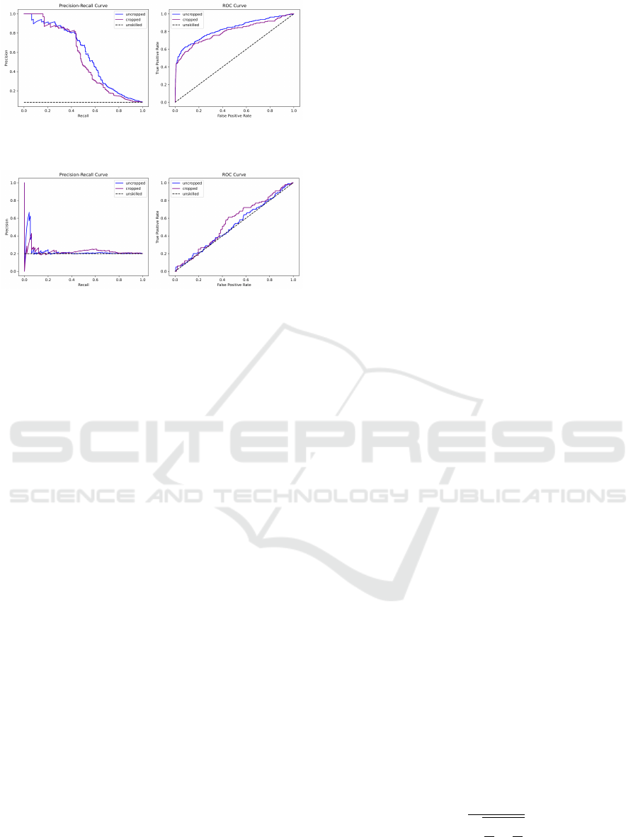
Figure 1: Evaluation results for two models trained and

evaluated on MIMIC-III. (Moazemi et al., 2022).

Figure 2: Evaluation results for two models trained on

MIMIC-III and evaluated on COPRA(Moazemi et al.,

2022).

prepared in the same way, and only those features

available in both datasets were used. The results

are presented in Figure 1 and Figure 2. Evaluating

the MIMIC-III-based model with the COPRA dataset

shows that the model is unable to make predictions on

a new independent dataset.

In this study, we compare both datasets to in-

vestigate possible differences in the data that can

explain the failure of generalization. We evaluate

whether there are minor differences between datasets

that could be solved by algorithmic solutions or if

generalization is a challenge that needs to be solved

by more complex solutions.

2 RELATED WORK

There is currently a vast amount of research regarding

machine learning in healthcare, but research into real-

world applications and arising challenges due to the

need for generalization is limited.

(Chekroud et al., 2024) evaluated a prediction

model for schizophrenia patients utilizing multiple

clinical trials and showed good accuracy for intra-trial

evaluations but failed for inter-trial evaluations. They

concluded that ﬁndings based on a single dataset pro-

vide limited insight into the general and future perfor-

mance of a model.

(Tonneau et al., 2023) have evaluated the general-

ization of a machine learning model in the domain

of radiomics. Although generalization results have

been improved by algorithmic solutions for one com-

bination of datasets, another combination of datasets

failed generalizability validations.

(Dexter et al., 2020) evaluated machine learning

generalization using free text laboratory data detec-

tion of speciﬁc diagnoses. Results show a signif-

icant decrease of model performance for inter-trial

evaluations, with the area under curve for the re-

ceiver operator characteristic as low as 0.48, indicat-

ing a model performance as good as guessing. They

concluded that “studies showing highly performant

machine learning models for public health analyti-

cal tasks cannot be assumed to perform well when

applied to data not sampled by the model’s train

dataset.”

Current research shows that while well-

performing models can be developed in healthcare,

generalization remains a challenge.

3 METHODS

Our goal was to evaluate the challenges of general-

izing machine learning methods in healthcare. To

achieve this, we conducted a comparative analysis be-

tween the COPRA database, used for evaluation in

(Moazemi et al., 2022) and the MIMIC III database.

The COPRA database includes 5,524 patient records,

while the MIMIC database contains 30,284 patient

records. Our analysis focused on two key aspects:

demographic information and time series data and the

differences of these features between the datasets.

3.1 Patient Demographics

We started with demographic data for age, height, and

weight retrieved from both databases. In this com-

parison, we analyze whether there were any signiﬁ-

cant discrepancies in the distribution of demographics

of the patients. We visualized the demographic dis-

tributions through KDE (Kernel Density Estimation)

plots. KDEs are a smoothed, continuous estimate of

the probability density function that describes the data

to compare distribution shapes and central tendencies

more easily between datasets.

To statistically assess any observed disparities, we

employed the following tests:

Welch’s t-test This test evaluates the signiﬁcance

of the difference between the means of two datasets.

The t-statistic is calculated as (WELCH, 1947):

t =

−

(1)

where

and

represent the sample means of the

two datasets, s

and s

are the sample variances, and

Challenges of Generalizing Machine Learning Models in Healthcare

255

and n

are the sample sizes of the two datasets.

This formula calculates how many standard devia-

tions the difference between the sample means is, pro-

viding a measure of the signiﬁcance of the mean dif-

ference.

Kolmogorov-Smirnov. This test assesses whether two

samples come from the same distribution. The K-S

statistic is deﬁned as (Massey, 1951):

D = sup

(x) − F

(x)

(2)

where F

(x) and F

(x) are the empirical cumulative

distribution functions of the two samples, and sup

denotes the supremum over all possible values of x.

The two statistical methods mentioned above are

a supplement to assess whether there are differences

between the distributions (apart from visual examina-

tion). The t-test is speciﬁcally designed to compare

the means of two groups and the K-S test compares

whether there are differences in the shape of the dis-

tributions, The K-S test does not assume a speciﬁc

distribution (like normality) and can be used with or-

dinal data or when the distribution of the data is un-

known.

3.2 Multivariate Time Series

We focused on Temperature, Oxygenation, Heart

Rate, and ambulatory blood pressure (ABP) for the

time series variables. To compute the distance be-

tween time series, evenly spaced time points are nec-

essary. Measurements are irregular across the original

datasets, hospital stays, features, and across time, as

they span from several minutes to hours. All time se-

ries data is resampled to a 15-minute sampling rate to

minimize the loss of information while regularizing

the time series. 15-minute bins are created through-

out the hospital stay, and the mean value of all values

in each bin is used for resampling.

We compared the time series data following two

complementary strategies:

First Strategy. We extracted all time series data for

each variable (e.g., temperature) from the COPRA

and MIMIC database and computed the following de-

scriptors: mean, standard deviation (std), trend, sea-

sonality, and cycle. These descriptors summarized the

central tendencies and temporal patterns within each

time series and are explained in Figure 3. To facili-

tate comparison, we plotted the distributions of these

descriptors for each variable, similar to our approach

to comparing patient demographics. This visualizes

any possible differences in the distribution of the vital

features and temporal patterns between the datasets.

Figure 3: Decomposition of a 48-hour vital sign time se-

ries into its components: cycle, trend, and seasonality. The

cycle refers to the longer-term oscillations within the data

that occur over an extended period, capturing patterns be-

yond daily or short-term ﬂuctuations. The trend represents

the overall direction or progression of the vital sign data

over time, whether increasing, decreasing, or remaining

constant. Seasonality highlights the recurring, predictable

patterns that repeat at regular intervals within 48 hours. To-

gether, these components help describe the structure of the

time series.

Second Strategy. We compared time series data us-

ing Dynamic Time Warping (DTW). DTW is a ro-

bust method for measuring the similarity between

two time series that may vary in speed or timing.

Given two time series, X = (x

, x

, ..., x

) and Y =

(y_1, y_2, ...., y

)where n and m represent the lengths

of the two-time series, DTW calculates an optimal

alignment between these sequences by minimizing

the cumulative distance (Müller, 2007).

The DTW distance is calculated by constructing

an n × m cost matrix C(i, j), where each element

C(i, j)represents the distance between points x

and

and is typically calculated as the squared Euclidean

distance:

C(i, j) = (x

− y

)

The goal is to ﬁnd a warping path W = (w

, w

, ...w

)

where each w

= (i

, j

) maps indices fromX to Y ,

that minimizes the total cumulative cost:

DTW (X,Y ) = min

(

∑

k=1

C(w

)) (3)

This optimal path minimizes the total distance by

allowing for shifts in time (i.e., stretching and com-

pressing of sequences) to better align the series. The

DTW distance provides a measure of similarity be-

tween the time series, with a lower DTW distance in-

dicating greater similarity.

Due to computational limitations, we computed

the DTW distance for a random subset of the data,

randomly sampling 1000 different data points from

each dataset for each vital feature (Temperature, Oxy-

genation, Heart Rate, and ABP). For example, we

measured the distance between 1000 temperature

time series from COPRA and 1000 temperature time

series from MIMIC.

HEALTHINF 2025 - 18th International Conference on Health Informatics

256

We created a DTW distance matrix between all

time series and plotted a heatmap to visualize any dif-

ferences between and in the two groups. This initial

analysis provided a broad and unbiased overview of

the similarities and differences between the datasets.

However, a high number of null values might impact

the DTW comparison. The reason is that all null

values are interpolated before calculating DTW dis-

tances, potentially misleading comparisons by com-

paring interpolation values (in case of many contin-

uous null values, e.g., a pattern line) rather than ac-

tual time series patterns. Recognizing this can lead to

misleading results due to the high proportion of null

values, we conducted a secondary analysis. This anal-

ysis involved ﬁltering out time series with more than

60 percent null values. In addition, we excluded time

series with fewer than 48 data points. We chose this

threshold because shorter time series might not cap-

ture enough temporal variation, something that is es-

sential for a meaningful DTW comparison.

4 RESULTS

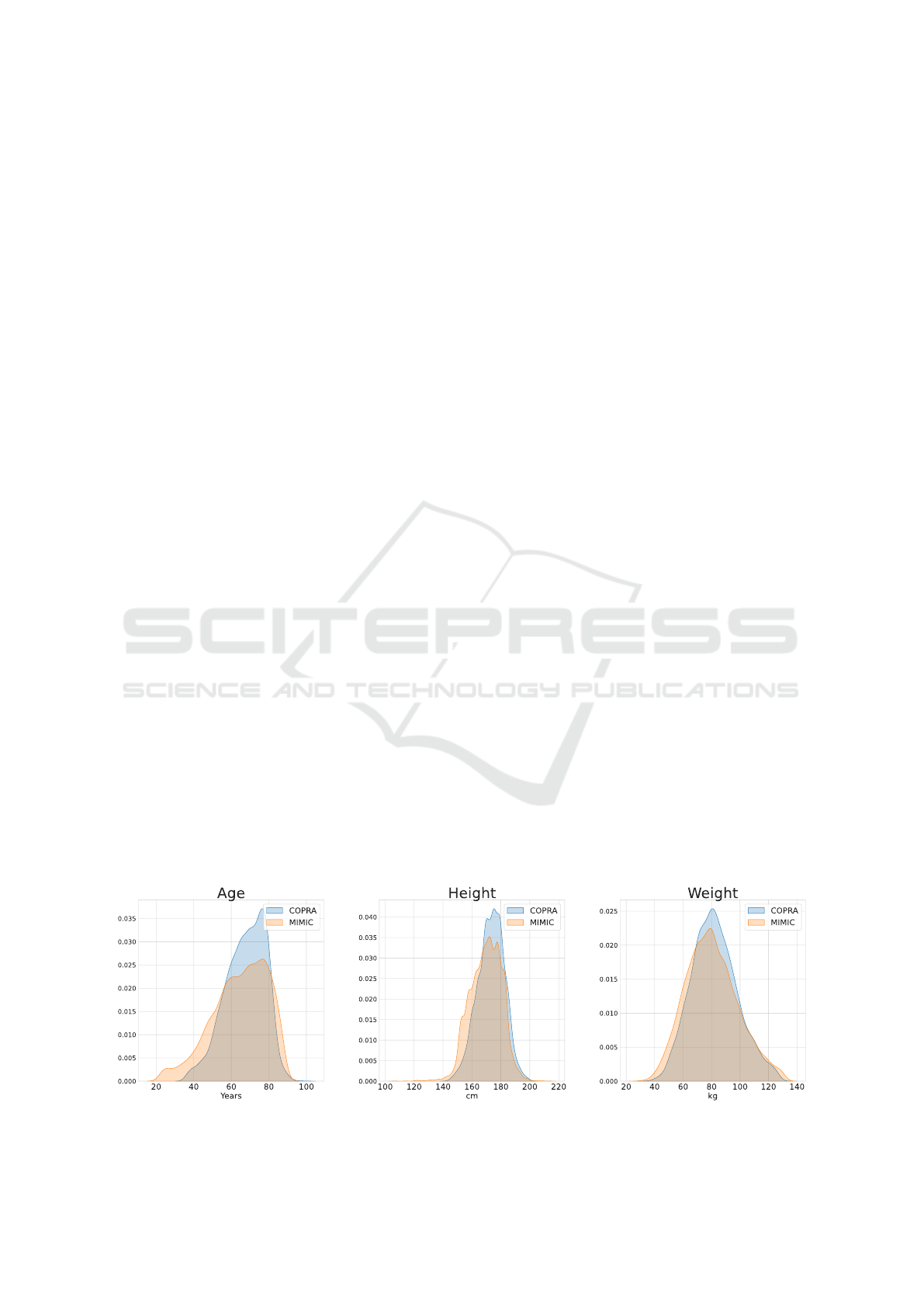
Figure 4 shows the comparison of demographic dis-

tributions of the variables age, height, and weight be-

tween COPRA and MIMIC datasets. The distribu-

tions of both datasets are overlapped to distinguish

the differences better. The distributions are approx-

imately normally distributed, although the age distri-

bution shows a skew towards higher values.

Table 1 shows the results of the t-test and k-test.

It shows signiﬁcant differences between the COPRA

and MIMIC datasets for age, height, and weight. The

large t-statistics tell us that these differences are not

just by chance; they are substantial. In particular,

height and weight show even bigger differences than

age. It is also important to note that the high t-values

are inﬂuenced by the large number of patient records

we compared. With such big groups, even slight dif-

ferences can become statistically signiﬁcant, so while

these differences are fundamental, the large sample

sizes make them stand out even more.

Figure 5 compares the time series descriptors for

Temperature, Oxygen, Heart Rate, and Arterial Blood

Pressure (ABP) between the COPRA and MIMIC

datasets. For each variable, violin plots display the

distribution of ﬁve key descriptors: mean, standard

deviation, trend, seasonality, and cycle. This visual

comparison helps us assess how consistent or variable

the time series data are across the two datasets.

The violin plots show the differences between

the two datasets across various descriptors. One of

the most striking differences is seen in the season-

ality of Temperature, where the median values for

COPRA and MIMIC are entirely different. More-

over, the cycles of the same variable are uniform in

MIMIC, whereas the COPRA dataset displays a pat-

tern with two distinct modes. These temperature vari-

ations could be due to differences in data collection

or processing methods used in the two datasets, or

they might reﬂect differences in patient populations

or conditions.

Figure 6 shows heatmaps of the distance between

time series computed via DTW. A majority of the

time series consists of mostly missing values due to

the resampling method and missing data. To calcu-

late the DTW, a linear interpolation is used to replace

the missing values. Due to computational limitations,

a subset of 2000 points from each dataset was used.

Brighter colors indicate a higher distance. The tem-

perature heatmap shows clearly that the distances in

the COPRA dataset are the lowest, and the distances

between COPRA and MIMIC are slightly higher than

the distances in the MIMIC dataset. There is no clear

visual difference for the other vital parameters.

To corroborate the visual results, the median dis-

tances are computed. The results are shown in Table

3. For Temperature and Oxygenation, the distance be-

Figure 4: Comparison of demographic distributions.

Challenges of Generalizing Machine Learning Models in Healthcare

257

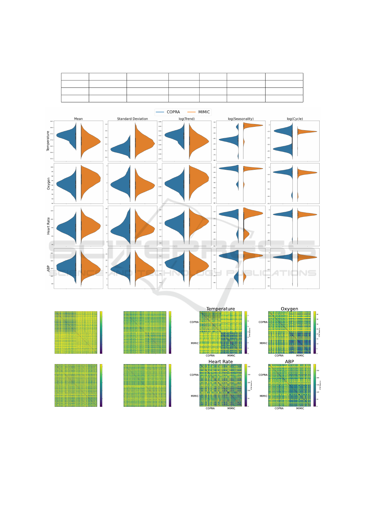
Table 1: Results of t-tests and Kolmogorov-Smirnov test comparing Demographic Variables Between the COPRA and MIMIC

Databases. All tests passed.

Variable Copra Mean MIMIC Mean t-Statistic p-Value K-S Statistic K-S p-Value

Age 66.83 62.02 13.39 < 0.001 0.26 < 0.001

Height 160.00 139.38 26.99 < 0.001 0.28 < 0.001

Weight 79.58 67.66 22.23 < 0.001 0.19 < 0.001

Figure 5: Comparison of time series descriptors across different variables.

COPRA MIMIC

COPRA

MIMIC

Temperature

COPRA MIMIC

COPRA

MIMIC

Oxygen

COPRA MIMIC

COPRA

MIMIC

Heart Rate

COPRA MIMIC

COPRA

MIMIC

ABP

DTW Distance

100

150

200

250

DTW Distance

100

150

200

250

300

DTW Distance

Figure 6: The DTW distances for vital values with 2000

data points from each data set.

Figure 7: The DTW distances for vital values. Only data

points with a limited number of missing values are depicted.

HEALTHINF 2025 - 18th International Conference on Health Informatics

258

tween COPRA and MIMIC is the highest, whereas,

for the other two features, the distance in the MIMIC

dataset is the highest. Due to the missing values, some

differences in the data might be unclear, as there can

be no new information obtained by comparing miss-

ing values against missing values.

Table 2: The median distances within and between datasets

with only data points with a limited number of missing val-

ues. The largest median distance for each feature is in bold.

COPRA MIMIC Mixed

Temperature 5.94 3.98 7.42

Oxygenation 32.16 18.15 33.38

Heart Rate 191.90 139.96 179.11

ABP 215.29 143.45 202.15

Table 3: The median distances within and between datasets.

The largest median distance for each feature is in bold.

COPRA MIMIC Mixed

Temperature 6.13 8.82 9.38

Oxygenation 26.63 26.60 29.23

Heart Rate 177.72 190.94 187.14

ABP 207.16 232.45 224.33

To obtain some more visual and precise numerical

results, we performed this analysis with time series

that consist of less than 60% missing values and at

least 12 hours of data. The results are shown in Fig-

ure 7 and Table 2. The higher inter-dataset distance is

more clearly visible for both Oxygenation and Tem-

perature. In Table 3, the effect of removing null values

can clearly be seen; the DTW mean distance within

the MIMIC group decreases, indicating that a large

number of null values can distort the results of DTW

calculations. On the other hand, the distances within

COPRA did not change signiﬁcantly, suggesting that

the analyzed COPRA dataset has higher-quality data

with fewer null values.

5 DISCUSSION

Differences in data are also evident in the distri-

bution of vital features, which cannot be attributed

solely to patient demographics and may instead stem

from variations in measurement techniques and clin-

ical protocols. This discrepancy is highlighted in our

DTW analysis, where Temperature and Oxygenation

show particularly high distances between the datasets.

(Lin et al., 2019) identify Oxygenation and Temper-

ature as critical for predicting patient readmissions

and suggest that substantial differences in these fea-

tures could impair model generalization. This ﬁnd-

ing indicates that there is no "free lunch" in machine

learning: models learn from and ﬁt to the data distri-

bution they are trained on, and they cannot generally

make reliable predictions for truly out-of-distribution

data. This also shows in the results of (Moazemi

et al., 2022): Slight differences in data would result

in less predictive performance, which could be im-

proved, e.g., by imputation methods. However, such

a failure to make correct predictions indicates that the

problem needs to be solved a step before: in data col-

lection and the construction of the model architecture.

To build general model architectures, these need

to be built with limitations of future datasets in mind -

if the architecture relies on relatively high availability

and quality of the data (which is available with pub-

lic datasets like MIMIC) it might not work for less

established datasets.

Another challenge arises from differences in miss-

ing values and sampling rates within and across

datasets. These variations complicate dataset com-

parisons and impact model performance. If a criti-

cal feature in a new dataset has a low sampling rate

or a signiﬁcant amount of missing data, it is unrealis-

tic to expect the model to utilize the data effectively,

even if it captures relationships in a more complete

dataset. Although algorithmic solutions such as impu-

tation can be helpful, they are no substitute for high-

quality data. Ultimately, creating more generalizable

models will require improvements in data quality and

availability.

6 CONCLUSION

By examining MIMIC-III and COPRA datasets, we

found signiﬁcant differences in demographic distribu-

tion and vital signs, which are likely to impact model

performance, limiting the efﬁcacy of models trained

on one dataset when applied to another. These ﬁnd-

ings highlight the need for models that not only pre-

dict accurately within a controlled setting but also

adapt to the diverse and evolving nature of real-world

healthcare data. Healthcare data is uniquely challeng-

ing due to its heterogeneity and how commonly data

is missing (Wells et al., 2013). Differences in clinical

practices, patient care protocols, and patient demo-

graphics between hospitals contribute to disparities in

datasets, which can alter model predictions and com-

promise patient outcomes. Such variations between

datasets make it clear that achieving generalizabil-

ity requires more than just reﬁning model architec-

tures. Algorithmic approaches like data imputation

and transfer learning can mitigate these issues but are

not sufﬁcient for data with stark differences. This im-

pacts machine learning in the domain of healthcare

Challenges of Generalizing Machine Learning Models in Healthcare

259

more than other domains, such as general natural lan-

guage processing, where large, well-curated datasets

are available.

As such, developing machine learning applica-

tions for healthcare needs more consideration. De-

veloping a machine learning model that makes cor-

rect predictions for one dataset might not be enough

to build general real-world applications. Overall, to

ensure the development and integration of machine

learning into healthcare applications, more collabo-

ration, more standards, and more data collection are

needed.

ACKNOWLEDGMENT

This research is funded by the German Federal Min-

istry of Education and Research (BMBF) under the

grant numbers 16KISR003 and 13GW0598C and by

the Susanne Bunnenberg Heart Foundation. We are

grateful for the funding received.

REFERENCES

Al-Zaiti, S., Martin-Gill, C., Zègre-Hemsey, J., Bouzid, Z.,

Faramand, Z., Alrawashdeh, M., Gregg, R., Helman,

S., Riek, N., Kraevsky-Phillips, K., Clermont, G., Ak-

cakaya, M., Sereika, S., Dam, P., Smith, S., Birnbaum,

Y., Saba, S., Sejdic, E., and Callaway, C. (2023). Ma-

chine learning for ecg diagnosis and risk stratiﬁcation

of occlusion myocardial infarction. Nature Medicine,

29:1–10.

Alaa, A. M., Bolton, T., Di Angelantonio, E., Rudd, J. H. F.,

and van der Schaar, M. (2019). Cardiovascular disease

risk prediction using automated machine learning: A

prospective study of 423,604 uk biobank participants.

PLOS ONE, 14(5):1–17.

Chekroud, A. M., Hawrilenko, M., Loho, H., Bondar,

J., Gueorguieva, R., Hasan, A., Kambeitz, J., Cor-

lett, P. R., Koutsouleris, N., Krumholz, H. M., Krys-

tal, J. H., and Paulus, M. (2024). Illusory gener-

alizability of clinical prediction models. Science,

383(6679):164–167.

Dexter, G. P., Grannis, S. J., Dixon, B. E., and Kasthuri-

rathne, S. N. (2020). Generalization of Machine

Learning Approaches to Identify Notiﬁable Condi-

tions from a Statewide Health Information Exchange.

AMIA Joint Summits on Translational Science pro-

ceedings. AMIA Joint Summits on Translational Sci-

ence, 2020:152–161.

Johnson, A., Pollard, T., and Mark, R. (2023). Mimic-iii

clinical database.

Kumari, J., Kumar, E., and Kumar, D. (2023). A structured

analysis to study the role of machine learning and deep

learning in the healthcare sector with big data analyt-

ics. Archives of Computational Methods in Engineer-

ing, 30(6):3673–3701.

Lin, Y.-W., Zhou, Y., Faghri, F., Shaw, M. J., and Campbell,

R. H. (2019). Analysis and prediction of unplanned

intensive care unit readmission using recurrent neu-

ral networks with long short-term memory. PloS one,

14(7):e0218942.

Massey, F. J. (1951). The kolmogorov-smirnov test for

goodness of ﬁt. Journal of the American Statistical

Association, 46(253):68–78.

Moazemi, S., Kalkhoff, S., Kessler, S., Boztoprak, Z., Het-

tlich, V., Liebrecht, A., Bibo, R., Dewitz, B., Licht-

enberg, A., Aubin, H., et al. (2022). Evaluating a

recurrent neural network model for predicting read-

mission to cardiovascular icus based on clinical time

series data. Engineering Proceedings, 18(1):1.

Müller, M. (2007). Dynamic time warping. Information

retrieval for music and motion, pages 69–84.

Panch, T., Mattie, H., and Celi, L. A. (2019). The “in-

convenient truth” about ai in healthcare. NPJ digital

medicine, 2(1):1–3.

Shapiro, D., Lee, K., Asmussen, J., Bourquard, T., and

Lichtarge, O. (2023). Evolutionary action–machine

learning model identiﬁes candidate genes associated

with early-onset coronary artery disease. Journal of

the American Heart Association, 12(17):e029103.

Tonneau, M., Phan, K., Manem, V. S. K., Low-Kam, C.,

Dutil, F., Kazandjian, S., Vanderweyen, D., Panasci,

J., Malo, J., Coulombe, F., Gagné, A., Elkrief, A.,

Belkaïd, W., Di Jorio, L., Orain, M., Bouchard, N.,

Muanza, T., Rybicki, F. J., Kaﬁ, K., Huntsman, D.,

Joubert, P., Chandelier, F., and Routy, B. (2023). Gen-

eralization optimizing machine learning to improve

CT scan radiomics and assess immune checkpoint

inhibitors’ response in non-small cell lung cancer:

a multicenter cohort study. Frontiers in Oncology,

13:1196414.

WELCH, B. L. (1947). The generalization of ‘student’s’

problem when several different population varlances

are involved. Biometrika, 34(1-2):28–35.

Wells, B. J., Chagin, K. M., Nowacki, A. S., and Kattan,

M. W. (2013). Strategies for Handling Missing Data

in Electronic Health Record Derived Data. eGEMs,

1(3):1035.

HEALTHINF 2025 - 18th International Conference on Health Informatics

260