Telosian: Reducing False Positives in Real-Time Cyber Anomaly
Detection by Fast Adaptation to Concept Drift
Iker Antonio Olarra Maldonado
1 a
, Erik Meeuwissen
1
, Puck de Haan
1
and Rob van der Mei
2 b
1
Cyber Security Technologies, TNO, The Hague, The Netherlands
2
Department of Stochastics, CWI, Amsterdam, The Netherlands
Keywords:
Anomaly Detection, Real-Time, Concept Drift, Unsupervised Learning, Intrusion Detection, False Positives.
Abstract:
We propose Telosian
∗
, an unsupervised anomaly detection model that dynamically adapts to concept drift.
Telosian uses a novel update scheme that measures drift and adapts the model accordingly. We show that
our update is faster than existing methods and results in an increased detection performance by reducing false
positives. In practice this will also reduce the workload of security teams. Moreover, through our experiments,
we show the importance of considering concept drift when deploying models. Further, the proposed model
is designed to be easily implemented in practice, taking into account the ease of deployment and reducing
operational costs without sacrificing detection performance. Additionally, we provide clear guidelines on how
such an implementation should be done. Moreover, we investigate the presence of drift in popular datasets
and conclude that the amount of drift is limited. We call on the academic community to develop more (cyber
security) datasets that capture drift.
1 INTRODUCTION
The development of effective intrusion detection sys-
tems plays a strategic role in safeguarding commer-
cial and military assets (Asif et al., 2013). Although
extensive research has been done in developing su-
pervised machine learning methods to perform this
task, several challenges prevent state of the art meth-
ods to be used in practice. The practical implica-
tions of deploying proposed methods are often over-
looked (Apruzzese et al., 2023b). These challenges
in implementation are related to: (1) The high cost
of labeling (Andresini et al., 2021), which makes
labeled data hard to procure (Tufan et al., 2021).
(2) The changes in the distribution of the data (con-
cept drift), which degrades the models’ performance
over time (Lu et al., 2018), and results in a constant
need to update deployed models. (3) The heteroge-
a
https://orcid.org/0009-0009-3665-6515
b
https://orcid.org/0000-0002-5685-5310
∗
The Telosian organ of cognition is housed inside a
segmented body that buds and grows at one end while with-
ering and shedding at the other. Every year, a fresh segment
is added at the head to record the future; every year, an old
segment is discarded from the tail, consigning the past to
oblivion. - Ken Liu, An Advanced Readers’ Picture Book
Of Comparative Cognition.
neous nature of networks, which makes the models
difficult to transfer from one environment to another
(Apruzzese et al., 2022), and finally (4) the high com-
putational and technical requirements of some meth-
ods (Apruzzese et al., 2023a).
Specially in Cyber Security, labeling observations
comes at a high cost (Andresini et al., 2021). In
(Apruzzese et al., 2022), it was seen that a company
can only afford to label 80 malware samples a day.
Furthermore, alarms must be reviewed constantly by
security analysts to stay up-to-date with the envi-
ronment and reduce false positives (Alahmadi et al.,
2022). These changes also produce label inaccuracy
due to label shift (Arp et al., 2022). Combined, these
factors could result in unreliable or outdated labeled
datasets. To mitigate these issues, anomaly detection
has become a central component in intrusion detec-
tion, as it can be used to develop more flexible and
efficient solutions to detect new attacks which pass
undetected to more traditional methods (Ahsan et al.,
2022). The importance of anomaly detection lies in
its flexibility to detect new outliers instead of learn-
ing specific cases (Zoppi et al., 2021). Besides, unsu-
pervised anomaly detection algorithms do not require
labeled datasets. This makes anomaly detection tech-
niques highly relevant when exploiting large amounts
of unlabeled data (Tufan et al., 2021).
84
Maldonado, I. A. O., Meeuwissen, E., de Haan, P. and van der Mei, R.
Telosian: Reducing False Positives in Real-Time Cyber Anomaly Detection by Fast Adaptation to Concept Drift.
DOI: 10.5220/0013320500003899
Paper published under CC license (CC BY-NC-ND 4.0)
In Proceedings of the 11th International Conference on Information Systems Security and Privacy (ICISSP 2025) - Volume 2, pages 84-97
ISBN: 978-989-758-735-1; ISSN: 2184-4356
Proceedings Copyright © 2025 by SCITEPRESS – Science and Technology Publications, Lda.

Furthermore, concept drift has been increasingly
identified as a main issue in the Cyber Security do-
main (Apruzzese et al., 2022), (Andresini et al.,
2021), (Arp et al., 2022). Concept drift occurs when
the underlying data distribution changes over time,
deviating from known patterns (Benjelloun et al.,
2019) and has been the cause of decreased perfor-
mance in many information systems, such as early
warning systems and decision support systems (Lu
et al., 2018). Nevertheless, the assumption that
data is stationary, independent and identically dis-
tributed is still prevalent in many methods (Andresini
et al., 2021), (Barbero et al., 2022), (Apruzzese et al.,
2023b). The only way of addressing concept drift is
through a constant update of the ML systems with
new data that reflects the current trends (Apruzzese
et al., 2023a). However, deciding when and how to
perform the update is difficult (Yang et al., 2021).
Additionally, systems become increasingly com-
plex and dynamic, which calls for more efficient and
flexible detection methods (Zoppi et al., 2021). Also,
the heterogeneity between environments makes trans-
fer learning hard; what is anomalous in one setting
could be normal in another one (Apruzzese et al.,
2022). This calls for models that are able to adapt
quickly to changes in the environment.
Finally, despite the advances in Machine Learn-
ing for intrusion detection, the proposed solutions
are seldom used in practice. For instance, in (Alah-
madi et al., 2022) only two out of 20 survey partic-
ipants reported using ML-based tools in their daily
operations. Oftentimes, proposed solutions focus on
benchmarks instead of building practical solutions
(Apruzzese et al., 2023b). This has led to large and
complex methods that are costly to maintain and op-
erate (Nadeem et al., 2023). For example, deep learn-
ing models have not shown a clear superiority over
existing methods while their cost and complexity is
evidently higher (Apruzzese et al., 2023a). There-
fore, there is need to develop effective solutions that
require few prerequisites, are easy to operate and are
able to perform in heterogeneous environments.
To address the challenges above, we propose
Telosian. A model that requires no labels and that is
designed to swiftly adapt when concept drift or sud-
den changes are present in the data, reducing false
positives. Additionally, it has few requirements mak-
ing it easy to implement in heterogeneous environ-
ments at a low cost. Our contributions are the follow-
ing:
• We propose an update scheme that leverages drift
measurement to dynamically adapt to different
kinds of drift.
• We introduce Telosian, a model that extends the
iForest algorithm by incorporating our proposed
update scheme, allowing it to dynamically adapt
to drift.
• We compare Telosian to BWOAIF (Hann
´
ak et al.,
2023), a state of the art model that adapts to drift.
We show that Telosian is able to reduce the num-
ber of false positives due to its dynamic adapta-
tion.
• We quantify the drift of existing benchmark
datasets and determine they have limited drift. We
make a call to the scientific community to gener-
ate more datasets that capture drift.
• We modify a real-world dataset to simulate drift.
The dataset can be used as a benchmark for drift
detection.
• To ensure the model’s applicability in practice,
we perform thorough experimentation on several
datasets, to study the effect of the model param-
eters and be able to provide clear guidelines for
deployment of the model in a new environment.
The remainder of the paper is organized as fol-
lows. In Section 2, we discuss anomaly detection
methods. We also introduce iForest. Then, in Sec-
tion 3 we explain the importance of addressing con-
cept drift and ways to detect it. We also describe the
NNDVI algorithm. Afterwards, in Section 4, we dis-
cuss the importance of considering drift when build-
ing anomaly detection models. We also introduce the
BWOAIF algorithm. Then, in Section 5, we present
Telosian. Subsequently, in Section 6, we describe our
experiment design as well as the SMD dataset used
for the experiments. Afterwards, in Section 7, we an-
alyze the experiments’ results and quantify the bene-
fits of dynamically adapting to drift. Finally, in Sec-
tion 8, we synthesize the results of the research and
the advantages of Telosian.
2 ANOMALY DETECTION
The goal of this research is to propose a method ca-
pable of performing unsupervised anomaly detection
in real-time streams of network data, taking concept
drift into account. In this section, we summarize some
of the proposed solutions to perform intrusion detec-
tion. First, we will discuss different anomaly detec-
tion methods and their application in the cyber secu-
rity domain. Then, we give a more in-depth expla-
nation of iForest, an accurate and efficient anomaly
detection algorithm.
The value of anomaly detection relies on the ca-
pacity to quickly identify anomalous patterns in data
Telosian: Reducing False Positives in Real-Time Cyber Anomaly Detection by Fast Adaptation to Concept Drift
85

without a need for previous knowledge of the na-
ture of the anomalous observations. Identifying these
anomalies reduces the amount of information that
needs to be carefully analyzed and results in a more
efficient use of resources. Anomaly detection is used
in multiple sectors. For example, in fraud detection,
anomaly detection is used to infer complexities and
dynamic changes in criminal behaviour (Gomes et al.,
2021), or in a military context, it is used on marine
traffic data to identify suspicious vessels (Bistron and
Piotrowski, 2021). In this section, we will discuss dif-
ferent methods that can be used to detect anomalies.
2.1 Anomaly Detection Methods
One of the challenges in anomaly detection is to de-
fine what normal behaviour entails. In this subsection
we will explore some of the methods that have been
proposed to detect anomalies. These methods can be
divided into the following main categories: density-
based methods, clustering methods, and isolation-
based methods (Benjelloun et al., 2019). All have
a different approach in identifying anomalies, which
can be useful in different contexts.
Firstly, clustering- and density-based anomaly de-
tection methods rely on the computation of distances
between data points in the feature space in order to
find patterns. Clustering methods partition the dataset
into groups, whose elements share similar character-
istics. Once the clusters are determined, points that do
not belong to any of these clusters or are the furthest
from them, according to a predefined metric, are la-
beled as anomalies (Zoppi et al., 2021). An example
of this approach is the k-Medoids algorithm, which
identifies anomalies by checking which points are fur-
thest from the central element of a cluster (Chitrakar
and Chuanhe, 2012). Density based methods, on the
other hand, group subsets of points that are close to
each other according to a chosen distance measure.
Then, the areas with lower density are used to find
anomalies (Togbe et al., 2020). The Local Outlier
Factor (LOF) algorithm (Breunig et al., 2000) is an
example of a density based method. Density-based
methods are more sensitive towards local outliers,
while clustering-based algorithms are more suited to
identify global anomalies (Benjelloun et al., 2019).
These approaches require pairwise distance calcu-
lation to compare the data instances, which makes
them ineffective in large datasets (Tufan et al., 2021).
These algorithms are still used in practice to this day,
for example in (Andresini et al., 2021), a Nearest Cen-
troid Neighbor classifier is used as a label estimator.
Contrarily, isolation-based methods rely on the as-
sumption that anomalies are few, different and that
the values of their attributes significantly differ from
those of normal instances of the data (Liu et al., 2008).
Hence, by separating the data based on individual at-
tributes, isolation-based methods can identify anoma-
lies without the need for computing distances, which
reduces their complexity and allows them to process
larger amounts of data (Togbe et al., 2020). In (Sid-
diqui et al., 2019), for example, the isolation-based
algorithm iForest was used to rapidly identify anoma-
lies in a database of over 300 million data instances,
which shows the scalability of this kind of method.
In the next section we discuss how anomaly detection
has been used in the cyber security context.
2.2 Anomaly Detection in Cyber
Security
In cyber security, anomaly detection has gained im-
portance as conventional methods have become in-
sufficient to detect the increasing number of incidents
(Ahsan et al., 2022). Although mechanisms to detect
known attacks are already present, such as rule-based
intrusion detection systems, these mechanisms lack
the flexibility needed to discover novel types of at-
tacks (Tufan et al., 2021). It has been recognized that
adequate cyber defense requires the capabilities of AI
to address the new threats that arise everyday (Lee-
nen and Meyer, 2021), (Layton, 2021). Algorithms
such as Random Forest, Naive Bayes and Neural Net-
works have been successfully utilized in the cyber se-
curity context. In (Ahsan et al., 2022) a summary of
the good performance of such algorithms on multiple
benchmark datasets is given. However, as stated be-
fore, high-quality labeled datasets are uncommon in
the cyber security field, which poses a major obstacle
for supervised algorithms. Existing labeled datasets
are often outdated or capture only a limited spectrum
of the cyber domain (Apruzzese et al., 2022). Ad-
ditionally, to make it possible for supervised algo-
rithms to detect new attacks, examples of them must
be recorded, labeled and used to retrain the algorithm.
This is time consuming and requires human labeling.
Semi-supervised methods have also gained impor-
tance recently. For example, insomnia (Andresini
et al., 2021) trains a model with an existing set of la-
beled data, the model then self-learns from the new
data by automatically labeling uncertain observations
with the aid of an assisting model (oracle). However,
this approach relies on the accuracy of the oracle. On
the other hand, new attacks could be labeled with high
confidence to an existing class, leading to misleading
results (Yang et al., 2021). Another example is (Sid-
diqui et al., 2019), where anomaly detection is com-
bined with expert feedback to increase accuracy and
ICISSP 2025 - 11th International Conference on Information Systems Security and Privacy
86

reduce the number of false positives in future runs.
Since unlabeled data is abundant in cyber secu-
rity, unsupervised methods are of particular impor-
tance. First, most of the publicly available datasets
in the cyber security domain have quality issues such
as lack of representation of existing attacks, class im-
balance and noisy or non-existent class labels (Ahsan
et al., 2022). Secondly, the continuous streams of data
require algorithms to be efficient and scalable. How-
ever, the assumption that anomalies are rare and show
deviating behavior holds for streaming data (Togbe
et al., 2020). This means that the traditional methods
could be adapted to process streaming data (Benjel-
loun et al., 2019). Few models are able to handle the
large amounts of data in combination with the neces-
sity for real time processing (Benjelloun et al., 2019).
Due to its scalability, efficiency and detection perfor-
mance, we consider iForest (Liu et al., 2008) to be an
ideal model to be extended to address concept drift.
The algorithm is explained in more detail below.
2.3 iForest
iForest (Liu et al., 2008), is an unsupervised ensem-
ble model designed to detect anomalies by isolation.
It uses recursive random partitioning of the data to de-
termine which instances are the most abnormal. It is
built under the assumption that anomalies are few and
different, and therefore easier to isolate than “normal”
instances of the data. The main advantages that make
iForest relevant for this research are: (1) its focus on
finding anomalies rather than profiling normal points,
(2) the fact that it does not require a labeled dataset
and (3) its high scalability (Liu et al., 2008). In this
section, we first explain the algorithm and then de-
scribe the characteristics that provide it with the afore-
mentioned advantages.
First, the algorithm is trained on a dataset of n
points where each point is composed of Q features
or attributes. To construct a single iTree, first, an at-
tribute is chosen from the data and then a random
split value is selected between the minimum and max-
imum value of this attribute. The split results in
two partitions of the original dataset which are subse-
quently divided by selecting another random attribute
and split value for each sub-dataset. This process is
repeated recursively until: (1) every partition reaches
a minimum size, or (2) a predefined number of splits
(iTree height) is reached. Following this process re-
sults in an iTree where the most anomalous points are
closer to the root of the tree. To build an iForest, T
iTrees are created from T independent samples of size
ψ taken without replacement of the dataset X . These
trees are used in an ensemble to assign an anomaly
score to each instance of the entire dataset X.
Once the trees are trained, the average path length
h
t
(x) of the point x across the iTree t ∈ {1, . . . , T } is
calculated. Then the average path length of an unsuc-
cessful search in BST is used to calculate the anomaly
score (Liu et al., 2008).
Despite its advantages, the algorithm is insuffi-
cient to address significant changes in the data (drift).
However, we can leverage its ensemble nature to per-
form partial updates of the model.
3 CONCEPT DRIFT
Concept drift refers to how the underlying distribu-
tion of the data changes over time and is one of the
main challenges in cyber security data (Layton, 2021)
(Andresini et al., 2021) (Arp et al., 2022). Address-
ing it is of paramount importance, as it can turn high-
performing models into outdated low-accuracy mod-
els. The only real way of addressing concept drift
is by continuously updating the model with data that
captures the new reality (Apruzzese et al., 2023a).
However, when and how to perform such task is not
trivial (Barbero et al., 2022).
Concept drift occurs in various ways. For ex-
ample, computer networks may present small grad-
ual changes due to an organic growth of the user
base, but also experience sudden changes caused by
a new type of attack. The different types of change
can be grouped in the following four categories: sud-
den drift, gradual drift, incremental drift and reoc-
curring concepts (Lu et al., 2018). In sudden drift
(Figure 1.a), the underlying distribution of the data
changes in a short period of time. Meanwhile, gradual
drift (Figure 1.b) occurs when the previous concept is
progressively replaced by the new one. Incremental
drift (Figure 1.c) is when the previous drift starts to
transform into the new one with a smooth transition.
Lastly, recurring concepts (Figure 1.d) refer to cases
where old concepts reoccur after some time. In cyber
security, both malicious and benign behavior experi-
ence drift, the former being sudden while the latter is
usually gradual (Andresini et al., 2021), (Apruzzese
et al., 2023a). It is important that models are able to
detect different kinds of concept drift in order to be
effective. In (Henriksen, 2023), for example, a model
trained to detect gradual and seasonal (reoccurring)
drift was shown to obtain better results than when
only one type of drift was considered. In the next
subsection, we will go through some methods used to
detect concept drift.
Telosian: Reducing False Positives in Real-Time Cyber Anomaly Detection by Fast Adaptation to Concept Drift
87

Figure 1: Types of concept drift (Lu et al., 2018).
3.1 Concept Drift Detection
There are a number of ways to detect concept drift,
however, most of the existing methods are supervised
approaches, which makes them unsuitable in sectors
where such data is scarce. For instance, in (Iwashita
and Papa, 2018), only two of the 59 surveyed methods
constitute unsupervised concept drift detection meth-
ods. We focused on unsupervised approaches, since
the implementation of supervised methods can be in-
feasible in cyber security application due to the lack
of reliable labels. Further, we identified three main
approaches to detect concept drift in an unsupervised
way: (1) assuming that drift exists, (2) tracking a spe-
cific statistic, and (3) measuring the discrepancies be-
tween batches of data.
The first approach simply assumes that concept
drift exists and periodically updates the model. This
approach is followed by (Tan et al., 2011) and (An-
dresini et al., 2021), where the model is updated with
every new batch or time window. Although simple
and effective, it can result in excessive training as
the models are replaced regardless of the existence of
drift and also, patterns learnt by the model could be
prematurely discarded.
On the other hand, the statistic tracking approach
consists of monitoring specific metrics of the model
to determine the existence of concept drift. When the
statistic changes significantly, an update is triggered.
In (Ding and Fei, 2013) and (Li et al., 2019), this
method is leveraged by tracking the average anomaly
rate of an anomaly detector. A more recent example
is (Yang et al., 2021), where a non-conformity mea-
sure is used to assess whether a record belongs to a
class. If this non-conformity measure is too big, then
it is assumed that drift is present. Nevertheless, this
approach is not effective for all types of concept drift
(Hann
´
ak et al., 2023) and relies on the accuracy of the
underlying model.
Finally, a more robust method relies on measuring
the differences between subsets of data. Samples are
taken from a reference batch and compared to samples
in a future window (Liu et al., 2018). This approach is
more sensitive to local drifts and is also application-
independent, because the subset can be taken from
any type of streaming data (Gemaque et al., 2020).
The NNDVI algorithm leverages this technique and is
explained below.
3.2 Nearest Neighbor-Based Density
Variation Identification
The NNDVI algorithm (Liu et al., 2018) compares
dissimilarities between samples taken from different
batches of the data. It has two main components:
a data modeling component, which builds a repre-
sentation of the data instances, and a distance func-
tion, which quantifies the dissimilarity between two
datasets. Below we elaborate on both components.
The data modeling component creates a repre-
sentation of the data to make different batches com-
parable (i.e., batches of data). NNDVI uses the Near-
est Neighbor-based Partitioning Schema (NNPS). The
schema groups similar data instances into partitions
and then compares the differences in density between
the partitions to asses their dissimilarity. The process
is similar to comparing two (high-dimensional) his-
tograms. NNPS, however, can be used for high dimen-
sional data and is more robust than other approaches
(Liu et al., 2018).
The NNPS assumes that closely located data in-
stances are related to each other. It expands each data
instance into a hypersphere like in Figure 2. In this ex-
ample, each point d
i
was expanded and this resulted in
three partitions p
i
. The intersection p
3
is the similar-
ity between the instances. For high-dimensional data,
NNPS defines the hyperspheres as multisets of parti-
cles. A multiset summarizes the relationship between
a set of particles and its k-nearest neighbors by tak-
ing into account the density of points around each in-
stance and the closeness with their neighbors. The as-
sumption is that if the distribution of the data changes
significantly, the closeness between neighbors and ar-
eas of density would change as well. Under this as-
sumption, a distance metric is used to compute the
similarity between two multisets, according to the in-
tersection between their elements.
Distance Function. To compare the multisets, a
weighted sum of the intersection between the hyper-
spheres of each element is computed. This distance
function follows a normal distribution, which allows
to perform z-test to assess the existence of drift.
Algorithm. The algorithm uses samples S
1
and S
2
from two datasets. Then, their corresponding multi-
ICISSP 2025 - 11th International Conference on Information Systems Security and Privacy
88

Figure 2: Example of hyperspheres and their intersection.
sets are obtained and the distance δ between the mul-
tisets is estimated. This process is repeated s times
with different samples to obtain an estimation of the
distribution of the distance. With this distribution, we
perform a statistical test on δ using a z-test. If the null
hypothesis (H
0
: “there is no difference between the
distance distribution of the samples”) is rejected, we
assume the existence of drift.
Apart from being an unsupervised algorithm,
NNDVI is robust to high dimensional data since data
instances are summarized into multisets. Also, ex-
panding the data instances into hyperspheres, makes
NNDVI more sensitive to changes in the distribu-
tion. Finally, the distance metric used to compare the
datasets returns a number between 0 and 1, which we
use to determine the size of update to be made. In
Section 5 we will explain how we use this to update
the initial ensemble.
4 NEED FOR DYNAMIC DRIFT
ADAPTATION
Existing techniques can benefit from awareness of the
observed drift. Which will allow the models to adapt
according to the type of change that is occurring in the
new data (Hann
´
ak et al., 2023). In Section 3 we listed
some examples of how models detect drift as well as
strategies of drift detection. In this section we will
motivate why measuring drift could be of great bene-
fit to improve their detection performance and explain
BWOAIF, a state of the art drift adaptating algorithm.
An initial idea to temper drift was to using traditional
models in sliding windows (Benjelloun et al., 2019),
allowing the algorithm to learn on the most up-to-
date data. In order to do this, many methods recre-
ate models from scratch every batch to stay up-to-date
(Hann
´
ak et al., 2023). Examples are the iForestASD
Figure 3: Update mechanism for the BWOAIF algorithm
with T = 8 trees and E = 2 new trees per batch.
algorithm (Ding and Fei, 2013) which trains a new
iForest algorithm every time concept drift is detected,
or the HS-Trees algorithm (Tan et al., 2011), which
resets the learnt parameters with every new batch of
data. This approach can be inefficient when concept
drift is small or nonexistent.
The BWOAIF algorithm (Hann
´
ak et al., 2023), on
the other hand, leverages the speed, scalability and
the ensemble nature of iForest to design a more effi-
cient method. This approach uses a sliding window
but only updates a fraction of the ensemble with ev-
ery batch, which improves accuracy and resource ef-
ficiency in comparison to existing methods such as
the iForestASD algorithm (Ding and Fei, 2013). This
state of the art model will be the baseline we will use
to compare Telosian. The BWOAIF algorithm is ex-
plained in the next subsection.
4.1 Bilateral-Weighted Online Adaptive
Isolation Forest
The Bilateral-Weighted Online Adaptive Isolation
Forest (BWOAIF) (Hann
´
ak et al., 2023) extends the
iForest algorithm to be used on streaming data. Its up-
date scheme allows it to deal with concept drift by
performing a partial update of the trees. The update is
done using non-overlapping data batches of size B and
replacing the oldest E trees with newly trained E trees
each batch. Figure 3 illustrates the process of tree re-
placement as new data arrives. Additionally, a weigh-
ing scheme is applied during the anomaly score cal-
culation. This results in an ensemble method where
the most recent iTrees have a stronger influence on
the computation of the anomaly score, thus allowing
it to deal with concept drift. In (Hann
´
ak et al., 2023),
it was shown that this constant retraining of the al-
gorithm resulted in higher accuracy and use of fewer
trees than other methods such as the iForestASD.
One of the limitations of this algorithm is that the
parameters that determine the speed of the update are
set at the beginning of execution. While the weighing
scheme and replacement of trees help the algorithm
address different types of concept drift
1
, with sud-
1
The algorithm includes a weighing method that allows
Telosian: Reducing False Positives in Real-Time Cyber Anomaly Detection by Fast Adaptation to Concept Drift
89

den drift only a predefined portion of the trees will
be trained on the new data. This can be an issue be-
cause, even if the obsolete trees are ignored, updated
trees might be too few to compute an adequate score.
On the other hand, with small or no concept drift, the
algorithm will still perform the same update size, re-
sulting in unnecessary computations. Our contribu-
tion is a new update scheme that is dependent on the
size of the concept drift. We believe that taking the
characteristics of the drift into account will improve
the performance of the algorithm.
5 TELOSIAN
The Telosian algorithm was designed to accurately
detect anomalies, and swiflty update according to
the amount of drift observed. Towards this goal,
Telosian uses three main components: (1) an en-
semble learner (iForest), (2) concept drift measuring
mechanism (NNDVI) and (3) an update scheme for the
ensemble model. These components allow the algo-
rithm to perform proportional and timely updates to
the model.
Figure 4 shows the process of the algorithm. Ini-
tially, the ensemble learner, which is trained with data
of previous batches, is used to predict the anomaly
scores (s
t
) of the current batch at time-step t. After-
wards, data is processed in batches performing four
main steps:
1. Concept drift is measured for the current batch us-
ing the NNDVI algorithm. The result is a value
ν
t
∈ [0, 1] which represents the drift.
2. The concept drift measurement is used to deter-
mine the proportion of the ensemble that should
be updated (E
t
: number of trees). This is done
using an update function explained later.
3. The update scheme, analogous to the one pro-
posed in the BWOAIF algorithm, replaces the E
t
oldest trees of the ensemble with newly trained
classifiers from the most recent data.
4. The new batch (t + 1) is processed with the latest
ensemble to predict the new anomaly scores, and
the process starts again.
To build the Telosian model, we make use of ex-
isting methods (iForest, BWOAIF and NNDVI) that
were explained in subsections 2.3, 3.2 and 4.1. In this
to give more or less influence to some trees and acceler-
ate or slow down the adaptation. However, the number of
replaced regressors, which constitute the basis of the algo-
rithm, remains constant
Figure 4: Components of the Telosian algorithm.
section we will further explain the role of each com-
ponent of the model, as well as the choice for methods
chosen for each task.
5.1 Initial Ensemble
The first step to build our model is training an ensem-
ble learner with existing static data. For this purpose,
we chose the iForest (Liu et al., 2008) algorithm, ex-
plained in subsection 2.3. The main advantages of the
algorithm are: its capacity to scale and its capacity
to detect multiple types of anomalies, without requir-
ing a labeled dataset (Liu et al., 2008). Despite these
advantages, the algorithm is not designed to handle
drift. However, iForest’s ensemble nature is compati-
ble with our proposed update scheme, to perform par-
tial updates of the model.
5.2 Concept Drift Measurement
The central component of our proposed model is the
measurement of concept drift, which allows us to de-
termine to what extent the model needs to be updated.
The Nearest Neighbor-Based Density Variation Iden-
tification (NNDVI) algorithm (Liu et al., 2018), ex-
plained in subsection 3.2, is of great use to achieve
this task. NNDVI can output a value ν ∈ [0, 1] depend-
ing on the amount of drift. We use this measurement
to determine the type of update that should be per-
formed on the model’s ensemble. Furthermore, the
algorithm is unsupervised, robust to high dimensional
data and more sensitive to changes in the distribution
in comparison to other methods (Liu et al., 2018).
5.3 Update Scheme
The next component of our proposed model is the up-
date scheme. This is what translates the drift mea-
surement into the number of trees to replace from the
ensemble. The proposed function takes the drift mea-
surement ν and outputs the number of trees to replace.
However, it is also important to see which trees are
to be replaced and how they are retrained. To per-
form this update, we use a schema similar to the one
proposed in the BWOAIF algorithm (Hann
´
ak et al.,
ICISSP 2025 - 11th International Conference on Information Systems Security and Privacy
90

2023), explained in subsection 4.1. In our approach
however, the parameter E that determines the num-
ber of trees to be updated is determined dynamically.
Below we explain how this update size is determined.
5.3.1 Tree Update Function
The tree update function translates the measurement
of concept drift into the number of trees to be re-
placed in the ensemble. The goal of the function is
to make the algorithm respond to different types of
drift by varying the update size. For example, when
drift is gradual or incremental, the function results
in small incremental changes, which maintain previ-
ously learnt patterns (iTrees), while slowly replacing.
When drift is sudden, on the other hand, the func-
tion will yield a large update so that the adaptation
is quick. Finally, the functions was defined to pre-
vent a full replacement of the ensemble in subsequent
batches, even with a maximum amount of drift. This
is useful for recurrent concepts where the data fluctu-
ates between different distributions. The function that
allows Telosian to accommodate changing drift is the
following:
τ(ν) = 2
⌊log
2
(νT )⌋
.
The function uses the drift score (ν) as argument.
The total number of trees T is also used
2
. A step func-
tion is used so similar concept drift results in a similar
update size. This also prioritizes small updates, but
allows for larger updates when the drift is high. The
chosen function will change at most half of the trees
to prevent over-fitting to a single batch.
Once the number of trees E to be updated is com-
puted, the scheme proposed in (Hann
´
ak et al., 2023)
for the BWOAIF algorithm is used. In this update
scheme, the oldest E trees are replaced by E new trees
trained on more recent data. Then, the data from the
new batch is given an anomaly score with the new
ensemble. Note that the bilateral weighing scheme
proposed in (Hann
´
ak et al., 2023) is also used.
Together, the previous steps allow the algorithm to
perform fast and proportional updates with respect to
the concept drift in the data.
6 EXPERIMENTATION
In this section, we describe how the Telosian algo-
rithm was tested. We compare Telosian with our own
implementations of the iForest and BWOAIF algo-
rithms. In the iForest case, our aim is to compare the
2
The number of trees T is considered a constant as it re-
mains unchanged throughout the execution of the algorithm
performance against an algorithm that does not con-
sider drift. On the other hand, we chose BWOAIF be-
cause it is a similar algorithm but, unlike Telosian, the
update size remains constant. This allows to evaluate
the effect of dynamically adapting to drift.
We used the Server Machines Dataset (SMD) (Su
et al., 2019) to complete the experiments. To measure
detection performance in unseen data, while still us-
ing that data for future updates, we make the batch
available for training, only after the algorithm has
made its predictions on it. To compare the algorithms,
we ran a grid search with more than 300 different
combinations of parameters for each algorithm. Then,
we used different thresholds to determine the param-
eter combination that maximized the F1-score.
6.1 Data
The data on which the algorithms are tested is highly
relevant. Unfortunately, there are few publicly avail-
able datasets for network intrusion detection, that cap-
ture drift (Maci
´
a-Fern
´
andez et al., 2018). We in-
vestigated the limited presence of drift by measur-
ing the amount of drift in existing datasets (see Ap-
pendix 5) using three different algorithms (NNDVI
(Liu et al., 2018), HDDDM (Ditzler and Polikar,
2011) and KdqTree (Dasu et al., 2006)). We con-
cluded that there is a gap in the literature for a real-
world network intrusion detection dataset that cap-
tures drift. Such a dataset would be of great impor-
tance for the development and testing of new algo-
rithms.
Nevertheless, we did identify the presence of drift
in the Server Machines Dataset (Su et al., 2019). For
this reason we chose it as the main dataset for our
experiments. Below, we describe some of the most
important characteristics of the chosen dataset.
Server Machines Data (Su et al., 2019). (SMD)
The dataset corresponds to the cyber security sec-
tor and consists of five weeks of data collected from
servers from an undisclosed large internet company.
The dataset contains labels for the anomalous records.
The labels will allow us to evaluate performance but
will not be used in the training the algorithm.
This dataset is comprised of 3 entities with 8, 9
and 11 machines respectively, for a total of 28 ma-
chines. This is the main dataset used for the research,
as it contains time dependent real world cyber secu-
rity data with various types of concept drift, making it
a suitable dataset to test the algorithms. This dataset
contains 38 features per observation, a total size of
1,416,825 observations (about 47,000 for every sub-
set) and an anomaly ratio of 2.08%
3
.
3
In the data repository a total of 4.16% is reported.
Telosian: Reducing False Positives in Real-Time Cyber Anomaly Detection by Fast Adaptation to Concept Drift
91

To be able to test the algorithms in a more re-
alistic setting, we opted to combine the sub-datasets
within each entity into a single dataset. This resulted
in one large dataset per entity (so three entity-datasets
in total) comprised of multiple weeks. Since all ma-
chines belong to the same entity, with similar behav-
ior, we aim to simulate different users the same ma-
chine. However, the anomalies seen in a machine will
be different from those seen on the other, thus simu-
lating zero-day attacks. We used the first two subsets
of each entity to train the initial ensemble and then
ran the algorithms on the remaining data.
6.2 Hardware Specifications
The experiments were run on the same server. The
server has 256GB of Memory, 32 cores and an In-
tel(R) Xeon(R) Gold 6244 CPU @ 3.60GH. The al-
gorithm was also deployed in a personal work sta-
tion with 16GB of Memory, 12 cores and an Intel(R)
Core(TM) i7-1255U processor to test its feasibility to
run in commodity hardware. The time performance is
reported in Appendix 9.
6.3 Algorithm Comparison Design
To compare the performance under various condi-
tions, we ran the algorithm with multiple parameter
configurations. The list below includes the subset of
parameters that were varied. The value of the rest of
the parameters was determined according to the best
practices stated in the literature. For instance, the
weighing of the anomaly scores of the BWOAIF al-
gorithm were set to σ
a
= 1000 and σ
v
= 0.05, follow-
ing the best practices stated in (Hann
´
ak et al., 2023).
Because Telosian uses a similar weighing scheme, we
used the same values.
• psi: The different values of subsampling which
will be used. The chosen values were {128, 256,
512}.
• ntrees: The different values for the number of
trees. The values used for the experiment are:
{256, 512, 1024, 2048}.
• n new trees: The different values for the number
of new trees. The values used for the experiment
are: {128, 256, 512, 1024}.
• batch size: The batch size to be used for the
streaming process. The batch sizes were selected
from the following values: {512, 1024, 4096,
8192, 16384}.
However, this proportion only considers the test set which
accounts for roughly 50% of the data.
This resulted in a total of |datasets| * |psi|
* |ntrees| * |n new ntrees| * |algorithms|
parameter combinations (1,008 valid combinations).
The best configuration (based on F1-score) was found
through a grid search. First, the initial ensemble was
trained over the two first sub-datasets of each entity.
Then, the rest of the entity-data was processed by
batches. In the case of the iForest, the ensemble re-
mains the same during the execution, while for the
other algorithms every batch was added to the slid-
ing window and used for training after the predictions
on the test set were computed. This way the labels
remain unseen to the algorithm during the anomaly
score computation phase. The final F1-score score
was computed using the predictions obtained during
every batch.
The metrics recorded during each execution were:
1. False Positive and False Negative count. To mea-
sure this we used four different cutoffs (0.5, 0.55,
0.6, 0.65, 0.7) for the anomaly score, to determine
which records are labeled as anomalies.
2. F1-score. The F1-score is the geometric mean
between precision and recall. It allows us to ac-
count for the imbalance of the dataset and gives
visibility on the errors of the dataset (Yang et al.,
2021).
3. AUC. Area Under the Receiver Operating Char-
acteristics curve (hereafter AUC). This metric
is more consistent than accuracy and makes it
easier to discriminate between classifiers (An-
dretta Jaskowiak et al., 2020). Additionally, it has
been widely used for iForest-related algorithms
(for example (Liu et al., 2008), (Hann
´
ak et al.,
2023), (Ding and Fei, 2013)).
4. Execution time. For every execution, the total
computation time and the time per batch were also
recorded.
7 RESULTS
In this section, we comment on the performance of the
three algorithms during the experimental phase de-
scribed in Section 6. First, we will present the overall
results obtained by the algorithms iForest, BWOAIF
and Telosian. After that, we analyze the performance
over time for the algorithms. Further, in Appendix
9 we discuss the effect of each hyperparameter on
Telosian with the goal of easing its implementation
in practice.
Table 1 shows the best AUC-ROC score obtained
after performing grid search for hyperparameter tun-
ing for all algorithms and entity-datasets. For each
ICISSP 2025 - 11th International Conference on Information Systems Security and Privacy
92

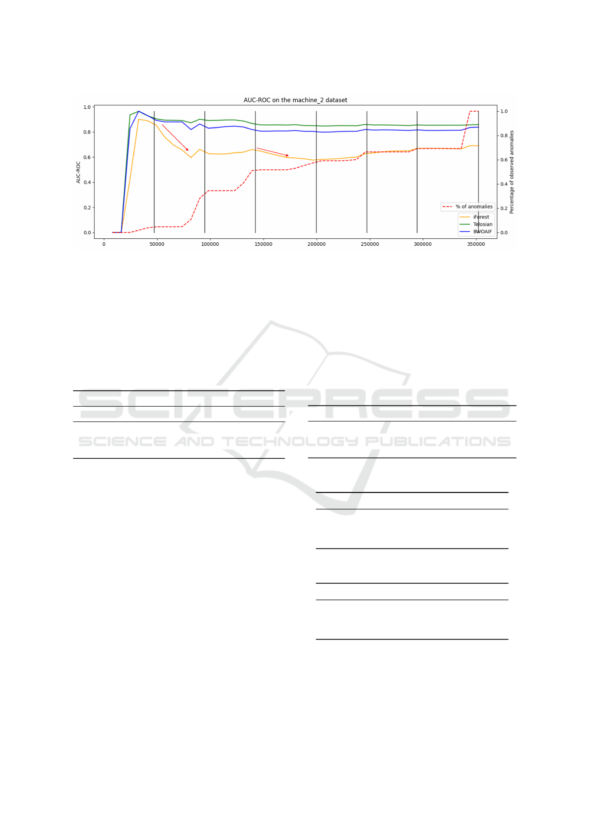
Figure 5: Cumulative AUC-ROC score for all three algorithms in machine 3.
dataset, the average drift score per batch is also
shown. An evident conclusion is that Telosian out-
performed the other algorithms. We can explain this
by two main reasons: first, the ability of Telosian to
adapt to new trends, and second, the speed at which it
performs this update. Below we further explain why
this occurs.
Table 1: Summary of the AUC scores of the three algo-
rithms on all entity-datasets.
Data Drift score AUC-ROC score
iForest BWOAIF Telosian
SMD1 0.776 0.804 0.804 0.808
SMD2 0.764 0.690 0.854 0.859
SMD3 0.677 0.646 0.782 0.795
Figure 5 shows the AUC-ROC score for all three
algorithms over time. The black vertical lines indicate
a change from one sub-dataset to another (i.e., a sud-
den change in the data). The red dotted line, shows
the accumulated (ground truth) anomalies until that
moment, which gives visibility on when the algorithm
should detect anomalies. From the figure, the ability
of both Telosian and BWOAIF to adapt to new trends
is evident, as they are able to maintain their perfor-
mance over time. iForest, on the other hand, exhibits
a decrease in performance. This is especially evi-
dent when changing from one sub-dataset to the other
(see red arrows). During these changes, we observe a
slight decrease in AUC from Telosian and BWOAIF,
followed by a recovery in performance. In contrast,
for iForest, there is a decay. This illustrates the im-
portance of including an update scheme to avoid de-
graded performance in the presence of drift. Now, we
will show how Telosian’s update scheme allows for a
better update than BWOAIF. The False Positive and
False Negative analysis is focused on BWOAIF and
Telosian. This is due to the greater number of mis-
classified records by the iForest algorithm (see Table
1), which would obfuscate the comparison between
Telosian and BWOAIF.
An initial observation from Table 1is the slightly
superior AUC scores of Telosian over BWOAIF. Ad-
ditionally, in Table 2 we also see similar performance.
However, we are interested in when the errors occur.
For this reason, we will analyze the false positives (ta-
ble 3) and false negatives (table 4) over time.
Table 2: F1-Score (Weighted F1-score).
Data Threshold BWOAIF Telosian
SMD1 0.60 0.248 (0.940) 0.230 (0.949)
SMD2 0.60 0.201 (0.963) 0.215 (0.968)
SMD3 0.65 0.174 (0.975) 0.176 (0.976)
Table 3: False Positives (FP).
Data Threshold BWOAIF Telosian
SMD1 0.60 15,616 9,403
SMD2 0.60 12,993 9,670
SMD3 0.65 7,282 7,159
Table 4: False Negatives (FN).
Data Threshold BWOAIF Telosian
SMD1 0.60 5,084 6,171
SMD2 0.60 3,610 3,846
SMD3 0.65 5,262 5,259
After analyzing the False Positives (FP) and False
Negatives (FN), we concluded that Telosian adapts to
new trends more quickly. This can be observed in Fig-
ure 6 which shows the FP generated by the algorithm
for entity-dataset 2. In the entity’s data, after every
sudden change (black vertical line), we observe an in-
Telosian: Reducing False Positives in Real-Time Cyber Anomaly Detection by Fast Adaptation to Concept Drift
93

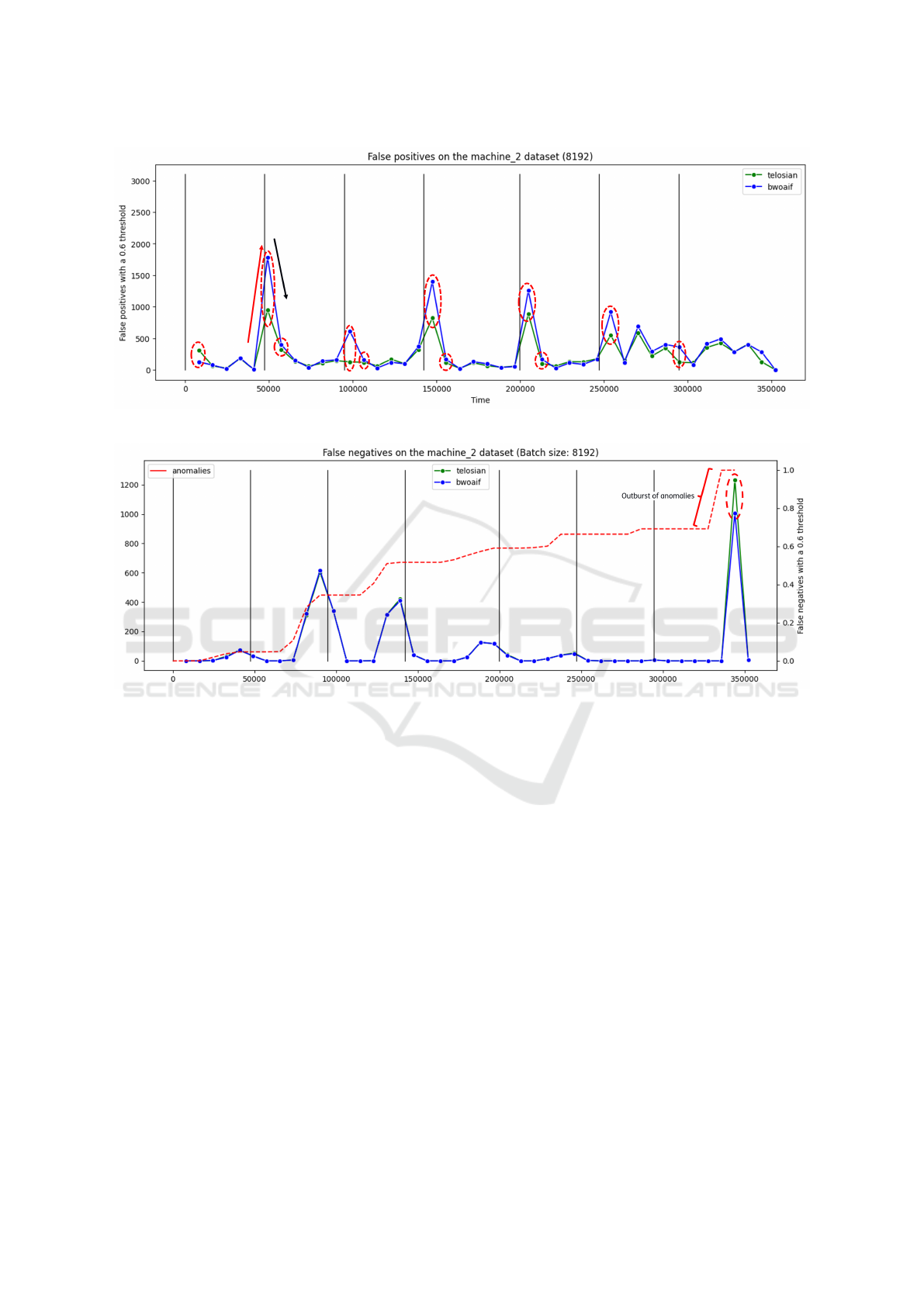
Figure 6: False positives per batch in machine 2.
Figure 7: False negatives per batch in machine 2.
crease the errors for both algorithms (this is shown
by the red arrow). After the initial increase in FP,
both algorithms detect the change in trend and adjust
accordingly, resulting in a detection performance re-
covery for the next batch (black arrow). This trend
repeats after every sudden change. Furthermore, the
errors produced by Telosian are fewer immediately af-
ter the update. The faster adaptation is also observed
in enitity-dataset SMD1 and SMD3, where Telosian
also produced fewer FP. A faster update is significant
advantage, as it allows it to ameliorate outbursts of FP
produced by changes in the distribution of the data. A
delayed response could be detrimental as real threats
could be concealed by large amounts of false alarms.
When analyzing false negatives, on the other
hand, we did not notice an evident difference in the
performance between BWOAIF and Telosian. In this
case, the fluctuations are more related to the appear-
ance of anomalies. In Figure 7, the red dotted line
shows how many of the total real anomalies present
in the data have been seen until that moment. The
solid lines show the FN for each algorithm. In the
Figure, we see an increase in FN correlated to the ap-
pearance of real anomalies (red dotted line). Telosian
produces slightly more FN in total. In figure 7, the
main difference in FN occurs when there is an out-
burst of anomalies. We can see in the graph that al-
most 30% of the anomalies occur in a small amount
of time. This also occurs in the other two datasets.
Since Telosian quickly adapts to new trends, when
many similar anomalies appear, the initial anomalies
will be detected. However, after some time Telosian
will stop seeing them as anomalies. In practice, this
is not necessarily undesirable, as the first anomalies
are flagged, giving time for the experts to investigate
them without generating repeated alerts for the fol-
lowing events.
Summarizing, the experiments showed a superior
overall performance of Telosian over BWOAIF, influ-
enced by the ability of Telosian to swiftly adapt to new
trends and thus generate fewer false positives after
sudden changes. However, a side effect are increased
false negatives when there is an outburst of anoma-
lies, This occurs because due to the fast adaptation,
ICISSP 2025 - 11th International Conference on Information Systems Security and Privacy
94

consequent anomalies may stop being flagged. How-
ever, as discussed in above, in practice this is not nec-
essarily undesirable. Further, the reduction of false
positives outweighs the slight increase in false nega-
tives. Additionally, comparing Telosian with a static
algorithm iForest, shows the importance of adding an
update scheme when addressing concept drift.
8 CONCLUSION
The goal of this research was to develop a model that
effectively detects anomalies, has minimal require-
ments and is able to address concept drift – one of
the main challenges when dealing with cyber security
data. We developed Telosian, an efficient, unsuper-
vised model that is able to adapt to changes in the
data in a swift manner.
Our experiments showed the importance of adapt-
ing to concept drift to maintain performance as well
as the impact of doing so in a swift way. Telosian’s
fast update allows it to reduce false positives specially
when sudden drift is present. However, a small in-
crease in false negatives could occur if an outburst
of anomalies is present. Nevertheless, this could be
solved by running another classifier in parallel. More-
over, Telosian is composed of scalable components
and only triggers updates when necessary, thus hav-
ing low computational requirements. Additionally, it
has a high detection performance without the need of
labels. These characteristics ease its implementation
in practice.
Finally, we investigated the presence of drift in ex-
isting datasets, concluding that current publicly avail-
able data for cyber security does not capture drift.
We make a call to the academic community to de-
velop more datasets that capture drift, as this is of
paramount importance in the development of novel
concept drift adapted methods.
9 FUTURE WORK
We identified some aspects of the algorithm which
could be investigated in future work to improve per-
formance. For instance, experiment with other algo-
rithms to measure and identify the type of drift. Ad-
ditionally, adding a functionality to temper outburst
of anomalies would add great value to the algorithm.
Furthermore, testing the algorithm on new cyber se-
curity datasets with labels for when drift occurs could
prove of great value. Finally, the trained trees could
be leveraged to try to explain the anomalies by us-
ing, e.g., information gain to determine which fea-
tures have a greater impact on a data instance being
an anomaly.
ACKNOWLEDGEMENTS
The work was partially funded by the European Union
– European Defence Fund under GA no. 101103385
(AInception). Views and opinions expressed are how-
ever those of the author(s) only and do not necessarily
reflect those of the European Union. The European
Union cannot be held responsible for them.
We would like to thank Dr. G
´
abor Horv
´
ath, one
of the authors of (Hann
´
ak et al., 2023), for his clari-
fications on the implementation of the BWOAIF algo-
rithm.
REFERENCES
Kdd cup 1999 data data set. Accessed: 2023-03-10.
Statlog (shuttle) data set. Accessed: 2023-03-10.
Ahsan, M., Nygard, K. E., Gomes, R., Chowdhury, M. M.,
Rifat, N., and Connolly, J. F. (2022). Cybersecurity
threats and their mitigation approaches using machine
learning—a review. Journal of Cybersecurity and Pri-
vacy, 2(3):527–555.
Alahmadi, B. A., Axon, L., and Martinovic, I. (2022).
99% false positives: A qualitative study of {SOC}
analysts’ perspectives on security alarms. In 31st
USENIX Security Symposium (USENIX Security 22),
pages 2783–2800.
Andresini, G., Pendlebury, F., Pierazzi, F., Loglisci, C., Ap-
pice, A., and Cavallaro, L. (2021). Insomnia: Towards
concept-drift robustness in network intrusion detec-
tion. In Proceedings of the 14th ACM workshop on
artificial intelligence and security, pages 111–122.
Andretta Jaskowiak, P., Gesteira Costa, I., and Jos
´
e
Gabrielli Barreto Campello, R. (2020). The area under
the roc curve as a measure of clustering quality. arXiv
e-prints, pages arXiv–2009.
Apruzzese, G., Laskov, P., Montes de Oca, E., Mallouli,
W., Brdalo Rapa, L., Grammatopoulos, A. V., and
Di Franco, F. (2023a). The role of machine learn-
ing in cybersecurity. Digital Threats: Research and
Practice, 4(1):1–38.
Apruzzese, G., Laskov, P., and Schneider, J. (2023b). Sok:
Pragmatic assessment of machine learning for net-
work intrusion detection. In 2023 IEEE 8th Euro-
pean Symposium on Security and Privacy (EuroS&P),
pages 592–614. IEEE.
Apruzzese, G., Laskov, P., and Tastemirova, A. (2022). Sok:
The impact of unlabelled data in cyberthreat detection.
In 2022 IEEE 7th European Symposium on Security
and Privacy (EuroS&P), pages 20–42. IEEE.
Arp, D., Quiring, E., Pendlebury, F., Warnecke, A., Pier-
azzi, F., Wressnegger, C., Cavallaro, L., and Rieck, K.
Telosian: Reducing False Positives in Real-Time Cyber Anomaly Detection by Fast Adaptation to Concept Drift
95

(2022). Dos and don’ts of machine learning in com-
puter security. In 31st USENIX Security Symposium
(USENIX Security 22), pages 3971–3988.
Asif, M. K., Khan, T. A., Taj, T. A., Naeem, U., and Yakoob,
S. (2013). Network intrusion detection and its strate-
gic importance. In 2013 IEEE Business Engineer-
ing and Industrial Applications Colloquium (BEIAC),
pages 140–144.
Barbero, F., Pendlebury, F., Pierazzi, F., and Cavallaro, L.
(2022). Transcending transcend: Revisiting malware
classification in the presence of concept drift. In 2022
IEEE Symposium on Security and Privacy (SP), pages
805–823. IEEE.
Benjelloun, F.-Z., Lahcen, A. A., and Belfkih, S. (2019).
Outlier detection techniques for big data streams: fo-
cus on cyber security. International Journal of Inter-
net Technology and Secured Transactions, 9(4):446–
474.
Bistron, M. and Piotrowski, Z. (2021). Artificial intelli-
gence applications in military systems and their in-
fluence on sense of security of citizens. Electronics,
10(7):871.
Breunig, M. M., Kriegel, H.-P., Ng, R. T., and Sander, J.
(2000). Lof: identifying density-based local outliers.
In Proceedings of the 2000 ACM SIGMOD interna-
tional conference on Management of data, pages 93–
104.
Chitrakar, R. and Chuanhe, H. (2012). Anomaly detection
using support vector machine classification with k-
medoids clustering. In 2012 Third Asian himalayas in-
ternational conference on internet, pages 1–5. IEEE.
Dasu, T., Krishnan, S., Venkatasubramanian, S., and Yi,
K. (2006). An information-theoretic approach to de-
tecting changes in multi-dimensional data streams. In
Proc. Symposium on the Interface of Statistics, Com-
puting Science, and Applications (Interface).
Ding, Z. and Fei, M. (2013). An anomaly detection ap-
proach based on isolation forest algorithm for stream-
ing data using sliding window. IFAC Proceedings Vol-
umes, 46(20):12–17.
Ditzler, G. and Polikar, R. (2011). Hellinger distance based
drift detection for nonstationary environments. In
2011 IEEE symposium on computational intelligence
in dynamic and uncertain environments (CIDUE),
pages 41–48. IEEE.
Gemaque, R. N., Costa, A. F. J., Giusti, R., and Dos San-
tos, E. M. (2020). An overview of unsupervised drift
detection methods. Wiley Interdisciplinary Reviews:
Data Mining and Knowledge Discovery, 10(6):e1381.
Gomes, C., Jin, Z., and Yang, H. (2021). Insurance fraud
detection with unsupervised deep learning. Journal of
Risk and Insurance, 88(3):591–624.
Hann
´
ak, G., Horv
´
ath, G., K
´
ad
´
ar, A., and Szalai, M. D.
(2023). Bilateral-weighted online adaptive isolation
forest for anomaly detection in streaming data. Statis-
tical Analysis and Data Mining: The ASA Data Sci-
ence Journal, 16(3):215–223.
Henriksen, A. (2023). Db-drift: Concept drift aware
density-based anomaly detection for maritime trajec-
tories. In 2023 Sensor Signal Processing for Defence
Conference (SSPD), pages 1–5.
Huasuya, T. (2019). Omnianomaly.
Iwashita, A. S. and Papa, J. P. (2018). An overview on con-
cept drift learning. IEEE access, 7:1532–1547.
Layton, P. (2021). Fighting artificial intelligence battles:
Operational concepts for future ai-enabled wars. Net-
work, 4(20):1–100.
Leenen, L. and Meyer, T. (2021). Artificial intelligence
and big data analytics in support of cyber defense. In
Research anthology on artificial intelligence applica-
tions in security, pages 1738–1753. IGI Global.
Li, B., Wang, Y.-j., Yang, D.-s., Li, Y.-m., and Ma, X.-
k. (2019). Faad: an unsupervised fast and accurate
anomaly detection method for a multi-dimensional se-
quence over data stream. Frontiers of Information
Technology & Electronic Engineering, 20(3):388–
404.
Liu, A., Lu, J., Liu, F., and Zhang, G. (2018). Accumulat-
ing regional density dissimilarity for concept drift de-
tection in data streams. Pattern Recognition, 76:256–
272.
Liu, F. T., Ting, K. M., and Zhou, Z.-H. (2008). Isolation
forest. In 2008 eighth ieee international conference
on data mining, pages 413–422. IEEE.
Lu, J., Liu, A., Dong, F., Gu, F., Gama, J., and Zhang,
G. (2018). Learning under concept drift: A review.
IEEE transactions on knowledge and data engineer-
ing, 31(12):2346–2363.
Maci
´
a-Fern
´
andez, G., Camacho, J., Mag
´
an-Carri
´
on, R.,
Garc
´
ıa-Teodoro, P., and Ther
´
on, R. (2018). Ugr ‘16:
A new dataset for the evaluation of cyclostationarity-
based network idss. Computers & Security, 73:411–
424.
Moro, S., R. P. and Cortez, P. (2012). Bank Market-
ing. UCI Machine Learning Repository. DOI:
https://doi.org/10.24432/C5K306.
Nadeem, A., Vos, D., Cao, C., Pajola, L., Dieck, S., Baum-
gartner, R., and Verwer, S. (2023). Sok: Explainable
machine learning for computer security applications.
In 2023 IEEE 8th European Symposium on Security
and Privacy (EuroS&P), pages 221–240. IEEE.
Quinlan, R. (1987). Thyroid Disease. UCI
Machine Learning Repository. DOI:
https://doi.org/10.24432/C5D010.
Siddiqui, M. A., Stokes, J. W., Seifert, C., Argyle, E., Mc-
Cann, R., Neil, J., and Carroll, J. (2019). Detecting cy-
ber attacks using anomaly detection with explanations
and expert feedback. In ICASSP 2019-2019 IEEE In-
ternational Conference on Acoustics, Speech and Sig-
nal Processing (ICASSP), pages 2872–2876. IEEE.
Su, Y., Zhao, Y., Niu, C., Liu, R., Sun, W., and Pei, D.
(2019). Robust anomaly detection for multivariate
time series through stochastic recurrent neural net-
work. In Proceedings of the 25th ACM SIGKDD inter-
national conference on knowledge discovery & data
mining, pages 2828–2837.
Tan, S. C., Ting, K. M., and Liu, T. F. (2011). Fast anomaly
detection for streaming data. In Twenty-second in-
ICISSP 2025 - 11th International Conference on Information Systems Security and Privacy
96

ternational joint conference on artificial intelligence.
Citeseer.
Togbe, M. U., Barry, M., Boly, A., Chabchoub, Y., Chiky,
R., Montiel, J., and Tran, V.-T. (2020). Anomaly de-
tection for data streams based on isolation forest using
scikit-multiflow. In Computational Science and Its
Applications–ICCSA 2020: 20th International Con-
ference, Cagliari, Italy, July 1–4, 2020, Proceedings,
Part IV 20, pages 15–30. Springer.
Tufan, E., Tezcan, C., and Acart
¨
urk, C. (2021). Anomaly-
based intrusion detection by machine learning: A case
study on probing attacks to an institutional network.
IEEE Access, 9:50078–50092.
Yang, L., Guo, W., Hao, Q., Ciptadi, A., Ahmadzadeh, A.,
Xing, X., and Wang, G. (2021). {CADE}: Detect-
ing and explaining concept drift samples for security
applications. In 30th USENIX Security Symposium
(USENIX Security 21), pages 2327–2344.
Zoppi, T., Ceccarelli, A., and Bondavalli, A. (2021). Unsu-
pervised algorithms to detect zero-day attacks: Strat-
egy and application. Ieee Access, 9:90603–90615.
APPENDIX
Drift in Popular Datasets
Table 5 shows the drift observed in six datasets. The
methods used for measuring drift compare consecu-
tive batches. However, the HDDDM (Ditzler and Po-
likar, 2011) and KdqTree (Dasu et al., 2006) are bi-
nary, so they only assess the existence of drift but not
its size. The number displayed on the table indicates
on which proportion of the batches drift was detected.
For NNDVI, on the other hand, the value displayed is
the mean amount of drift measured in each batch.
Effect of Hyperparameters on Telosian
The grid-search approach to find the best combina-
tion of hyperparameters also gives more visibility on
the effect of changing a specific parameter on the
accuracy of the model for each dataset. The purpose
of this section is to explain the found trends and give
Figure 8: The effect of changing the number of trees (T )
and sub-sampling size (ψ) in the processing time per batch.
guidelines to set the hyperparameters.
Effect of the Number of Total Trees. (T ) We
advise to use values slightly below 500 for Telosian
to balance detection performance and computational
efficiency.
Effect of the Subsampling Size. (ψ) We recom-
mend using values of 1000 or greater for Telosian.
However, if the number of attributes is small, values
of ψ around 250 should be used.
Effect of the Batch Size. We advise to use 600 to
2500 records per batch, but the user should adjust this
depending on the business logic.
Processing Time per Second
For most parameter combinations, Telosian is able to
process 100 records in less than 1 second. This pro-
cessing time includes the training of new trees, mea-
suring of drift and the computation of the anomaly
scores. Furthermore, specific combinations of param-
eters take less than 0.2 seconds, which shows that
changing the parameters of the algorithm could fur-
ther reduce run times.
Figure 8 shows that the algorithm scales linearly
with the number of records and that even with a large
number of trees and sub-sampling size, which makes
it a feasible option for a real-time use case.
Table 5: Measured drift in the datasets using multiple methods.
Dataset NNDVI HDDDM KdqTree
SMD (Huasuya, 2019) 0.73 0.148 0.988
KDDCUP Http (kdd, ) 0.28 0.209 0.001
KDDCUP Smtp (kdd, ) 0.17 0.276 0.459
Thyroid disease (Quinlan, 1987) 0.18 0.231 0.077
Bank marketing (Moro and Cortez, 2012) 0.13 0.062 0.012
Shuttle (shu, ) 0.13 0.084 0.0
Telosian: Reducing False Positives in Real-Time Cyber Anomaly Detection by Fast Adaptation to Concept Drift
97