Skeleton-Based Bilateral Symmetry: Theoretical Concepts and Detection
via Dynamic Programming
Nikita Lomov
a
, Oleg Seredin
b
and Olesia Kushnir
c
Tula State University, Prospekt Lenina, 92, Tula, 300012, Russia
Keywords:
Skeleton, Bilateral Symmetry, Medial Representation, Jaccard Index, Dynamic Programming.
Abstract:
This study presents a formal definition and an algorithm for the detection of bilateral symmetry in flexible
planar objects. We proposed to analyze the skeleton of a 2D figure and detect its symmetry using the auto-
morphism of the original and reflected skeleton graphs enhanced with additional requirements. The axis of
symmetry is formed by the skeleton edges invariant under reflection. We developed a dynamic programming
algorithm that finds the optimal mapping of the half-edges of the skeleton considering their “duality”. We
also implemented a symmetrization of the skeleton and original figure, making the detected axis the figure’s
vertical axis of reflective symmetry. We showed that the optimized target value when searching for the skeletal
mapping agrees well with the Jaccard similarity index.
1 INTRODUCTION
Symmetry is an important feature of many objects
perceived by human vision. Symmetry detection
tools are important for many computer graphics and
computer vision applications such as morphing, ob-
ject classification, style transfer, parametrization, etc.
Apart from the intuitive concept of symmetry as
“something composed of identical elements” or “self-
similar”, symmetry is a meaningful mathematical
concept. It implies the existence of a transformation
that does not change the object’s shape when its parts
are rearranged. The simplest examples are reflection
and rotation. The points invariant to such transforma-
tions (the axis of reflection and the center of rotation)
are called the center of the object.
Symmetry detection is complicated for real-world
objects captured by cameras, scanners, and sensors.
First, the transformation becomes rather complex.
Second, even when the formal transformation applies,
complete self-similarity of the object is impossible.
The first aspect is mostly attributed to the fact that
real-world shapes are at least partly flexible, so the
axis of symmetry is curvilinear; besides, segments of
many living beings can articulate independently of the
major axis. Human arms are a good example of this.
As a result, the definition of symmetry through only
a
https://orcid.org/0000-0003-4286-1768
b
https://orcid.org/0000-0003-0410-7705
c
https://orcid.org/0000-0001-7879-9463
one axis is insufficient. We need to specify how the
pairs of the object points map onto each other.
The symmetry of a planar figure requires a pair-
wise correspondence between all the points of the fig-
ure. Any planar shape can be represented by a set
of lines with non-zero thickness and is completely
“packed” into a skeleton, a set of its skeleton axes.
The skeleton of a 2D figure is a planar graph, so we
can apply the well-developed graph theory to the sym-
metry analysis.
The purpose of this study is to rigorously formal-
ize the concept of planar graph symmetry and develop
a symmetry detection algorithm. The proposed algo-
rithm can be applied to the analysis of planar figures
defined as their medial representations to evaluate the
degree of symmetry and symmetrization. Our exper-
iments show that the proposed symmetry index cor-
relates well with the Jaccard index of the figure after
symmetrization. The algorithm is versatile and offers
high computational efficiency.
2 RELATED WORK
The simplest type of bilateral symmetry that requires
a nontrivial deformation of the figure is curvilinear
symmetry. It is completely defined by the equation of
its axis. A method for detecting all possible curvi-
linear axes approximated by polylines using a dy-
namic programming algorithm is proposed in (Lomov
746
Lomov, N., Seredin, O. and Kushnir, O.
Skeleton-Based Bilateral Symmetry: Theoretical Concepts and Detection via Dynamic Programming.
DOI: 10.5220/0013321400003912
Paper published under CC license (CC BY-NC-ND 4.0)
In Proceedings of the 20th International Joint Conference on Computer Vision, Imaging and Computer Graphics Theory and Applications (VISIGRAPP 2025) - Volume 3: VISAPP, pages
746-754
ISBN: 978-989-758-728-3; ISSN: 2184-4321
Proceedings Copyright © 2025 by SCITEPRESS – Science and Technology Publications, Lda.

and Seredin, 2023). A greedy algorithm for tracing
a curvilinear symmetry axis is proposed in (Seredin
et al., 2023). It aims to pass the points with the best
local symmetry along the normal to the path. A graph-
based algorithm is used in (Liu and Liu, 2011) to con-
struct the symmetry axis as a polyline for the full-
color image region so that the characteristic of the
polyline at each point is the spread (the length of the
symmetric perpendicular section).
In (Huang et al., 2023), a planar shape is repre-
sented by a polygon for which an integer program-
ming algorithm finds the optimal mapping of the
sides.
An approach that reduces the symmetry detection
problem to mapping chains of skeleton primitives is
discussed in (Kushnir et al., 2017). The properties of
skeleton edges are length, angle of rotation relative to
the previous edge (in the order of traversal), and the
width of the figure along the edge. For the efficiency
of comparison, the width is defined by the Legendre
polynomial’s coefficients.
In (Qian et al., 2015), the authors consider the
main chain of the skeleton as the axis of curvilinear
symmetry and introduce a mutual correspondence be-
tween the terminal vertices of the skeleton and the
chains connecting these vertices. The properties of
the vertices are the distances to the axis, the proxim-
ity of their joint points, and the width of the figure in
the vicinity of the point. The edges are defined by the
ratio of geodesic distances between their ends. A ge-
netic algorithm is used to find the optimal mapping.
For symmetrization, the shape width between the cor-
responding branches of the skeletal graph is averaged.
The method proposed in (Yang et al., 2008) di-
vides the contour into two parts. They are compared
using the distribution of geodesic distances between
their critical points measured along the contour. A
similar approach is used in (Bai and Latecki, 2008) to
compare two different shapes for image classification.
The distances are measured along the skeleton edges.
Note that the methods analyzing the distribution
of skeletal distances can be generalized to 3D shapes
and therefore are quite popular. In (Wang et al.,
2019), skeletons are used to map convex shape frag-
ments that have extrinsic symmetry, ultimately defin-
ing intrinsic symmetry. Another area of research
is the analysis of 3D skeletons represented by point
clouds (Jiang et al., 2013) or triangular meshes (Na-
gar and Raman, 2018). Reflective symmetry of rigid
3D shapes is studied in (Cicconet et al., 2017) in terms
of the point cloud mapping problem. Methods for di-
rect analysis of 3D skeletons with various representa-
tions are developed in (Song et al., 2018; Huang et al.,
2013).
Self-symmetry of the shape can be an issue be-
cause the dual points have similar properties. This
drawback is analyzed in (Xu and Zhang, 2016) as ap-
plied to human 3D skeletons. The symmetry of many
organic shapes is analyzed in (Li et al., 2019) to map
the parts of two symmetrical shapes (such as animal
figures). For this, an axis of symmetry is detected
in each skeleton by comparing subgraphs connected
to the axis candidate, and subgraphs of the different
shapes with similar intrinsic properties are compared.
A correspondence between two symmetric 3D shapes
is sought in (Liu et al., 2012), but the symmetry is
defined by a closed curve on the surface.
However, the proposed methods do not allow one
to directly derive a normalized and well-interpretable
measure of symmetry for 2D shapes.
3 PLANE SHAPE SKELETONS
It is reasonable to digitally represent the shape of ob-
jects as binary raster images. However, we consider
continuous skeletonization resulting in planar shapes
and skeletons represented as parametric curves, since
this is much more convenient for analytical process-
ing.
A figure is a closed region bounded by a finite
number of non-intersecting Jordan curves. The skele-
ton S of a figure A is the closure of the set of shape
points having several nearest boundary points. The
radial function r(c) : S → R
+
takes the value of the
radius of the largest circle centered at s and inscribed
in the shape. We will denote the circle as B(c). The
skeleton and radial function combined are called the
medial representation. We will also define a silhou-
ette H(S
′
) for the skeleton’s fragment S
′
⊆S: H(S
′
) =
∪
c∈S
′
B(c). Since A = H(S), a conversion to the me-
dial representation allows us to completely recon-
struct the original shape and preserves all the shape
information.
The medial representation exists for all planar
shapes, but for real-life applications, it is convenient
to restrict the range of shapes to polygonal shapes
whose boundaries are simple polygons. In this case,
the skeleton consists of a finite number of straight
and parabolic segments, while the radial function has
a simple analytic form. Any shape can be approxi-
mated by a polygon with sufficient accuracy. Since
the skeletons may have many occasional edges, a
pruning procedure is used to simplify the skeleton by
removing the edges that have little effect on the sil-
houette. The basic concepts of skeletons are shown in
Fig. 1.
To approximate the shape of binary image objects
Skeleton-Based Bilateral Symmetry: Theoretical Concepts and Detection via Dynamic Programming
747

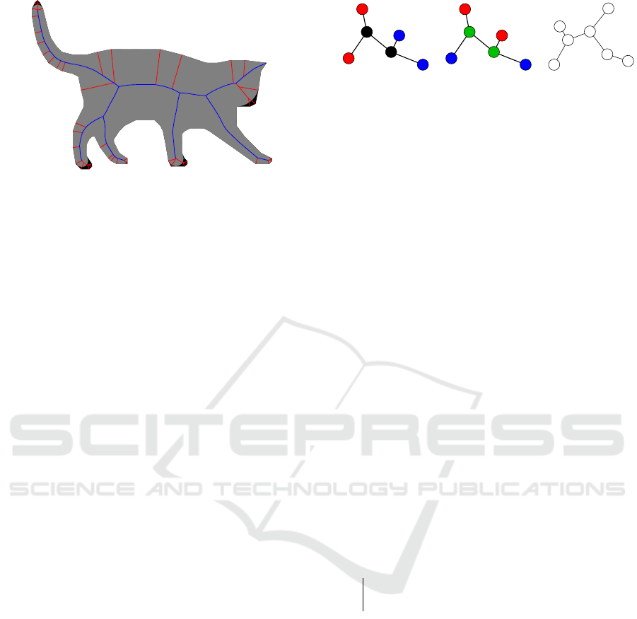
Figure 1: Skeleton of a planar shape approximated by a
polygon. Red: branches removed by pruning. Blue: re-
maining branches. Grey: their silhouette. Black: part of the
shape lost due to pruning.
with polygonal figures and calculate their skeletons,
we used the algorithms described in (Mestetskiy and
Semenov, 2008; Mestetskiy and Koptelov, 2024). It
is reasonable to consider that for a shape with some
symmetry its skeleton graph is also symmetric. The
formalization of planar graph bilateral symmetry will
be discussed below.
4 DEFINITION OF SKELETAL
SYMMETRY
Let us consider an undirected planar graph G =
(V, E). It has reflective symmetry, if there exists
a rectilinear planar embedding g : V → R
2
, g(u) =
(x(u), y(u)), which is symmetric about Y -axis:
∀(u, u
′
) ∈ E ∃(v, v
′
) ∈ E :
g(v) = (−x(u), y(u)), g(v
′
) = (−x(u
′
), y(u
′
)).
We will consider the vertices for which x(u) < 0
to be left ones and belonging to the set L. The set
of right vertices R contains the vertices for which
x(u) > 0. Finally, the vertices with x(u) = 0 consti-
tute the set of center vertices C . Then we can define
the symmetry in terms of the graph itself: there exists
an automorphism f : V →V such that:
1. f (u) = v =⇒ f (v) = u,
2. u ∈L =⇒ f (u) ∈ R ,
3. (u, v) ∈E and u ∈ L and v ∈ R =⇒ f (u) = v,
4. We cannot move any elements from C to L and R
keeping the above properties intact.
Note that the contrary is also true: if such an auto-
morphism exists, then the corresponding planar em-
bedding also exists.
Examples of symmetric and asymmetric graphs
are shown in Fig. 2. Note that the symmetrizing au-
(a) (b) (c)
Figure 2: Symmetric (a,b) and non-symmetric (c) graphs.
Pairs of vertices with the same color are symmetric to each
other. Black vertices map into themselves.
tomorphism f can be defined in multiple ways and
specify various axes of symmetry.
5 SEARCH FOR OPTIMAL
SKELETAL SELF-MATCHING
Let us construct a connected, undirected, acyclic
planar graph G = (V, E) with half-edges
ˆ
E =
S
(u,v)∈E
{u → v, v → u}. Using a planar embedding
of graph G, for each vertex u and its incident vertex
v, we can create a function next
v
(u) : V → V , which
defines the final vertex of the edge v → u
′
following
counterclockwise the edge v → u. Then, starting from
an arbitrary half-edge e ∈
ˆ
E, we can find a unique or-
der of traversal for the graph G (Algorithm 1). As a
result, the list T will contain all 2|E| half-edges of G
without repetitions.
Data: Graph
ˆ
G = (V,
ˆ
E), embedding g
Result: Traversal T
Choose any e ∈
ˆ
E;
T = [];
e
0
= e;
do
T .append(e);
e = v → next
v(e)
(u(e));
while e ̸= e
0
;
Algorithm 1: Planar graph traversal.
Let us symmetrically reflect the embedding of the
graph G. Then during its traversal, the next clock-
wise edge will be previous in the original embedding.
Therefore, a new traversal T
′
can be obtained by ar-
ranging the edges in T in reverse order.
Let T = [t
1
,t
2
, . . .t
n
], T
′
= [t
′
1
,t
′
2
, . . .t
′
n
], and a func-
tion p defines the index of the twin half-edge: t
i
=
u → u
′
, t
j
= u
′
→ u =⇒ p(i) = j. The function
p
′
(i) is defined similarly. For a symmetric graph G,
we construct a one-to-one correspondence s between
the elements of T and T
′
: for f (u) = v, f (u
′
) = v
′
,
t
i
= u → u
′
, t
′
j
= v → v
′
, s(i) = j. The opposite is also
true: we can restore the automorphism f from that
VISAPP 2025 - 20th International Conference on Computer Vision Theory and Applications
748

Data: Traversals T , T
′
, |T | = n, |T
′
| = m
Function align(i
1
, i
2
, j
1
, j
2
)
if R(i
1
, i
2
, j
1
, j
2
) ≥ 0 then
; // do nothing
end
else if j
1
> j
2
then
r = 0; //
e
T
′
is empty
for i = i
2
, . . . , i
1
do
r = r + w
i0
;
R(i, i
2
, j
1
, j
2
) = r;
B(i, i
2
, j
1
, j
2
) = 1;
end
end
else if i
1
> i
2
then
r = 0; //
e
T is empty
for j = j
2
, . . . , j
1
do
r = r + w
0 j
;
R(i
1
, i
2
, j, j
2
) = r;
B(i
1
, i
2
, j, j
2
) = 2;
end
end
else
d = [w
i0
+ align(i
1
+ 1, i
2
, j
1
, j
2
),
w
0 j
+ align(i
1
, i
2
, j
1
+ 1, j
2
)];
if p(i
1
) > i
1
then
d.append(2w
i
1
j
1
+ align(i
1
+
1, p(i
1
) −1, j
1
+ 1, p
′
( j
1
) −1) +
align(p(i
1
)+1, i
2
, p
′
( j
1
)+1, j
2
);
end
R(i
1
, i
2
, j
1
, j
2
) = mind;
B(i
1
, i
2
, j
1
, j
2
) = argmind;
end
return R(i
1
, i
2
, j
1
, j
2
);
end
Algorithm 2: Calculation of the symmetry functional as the
similarity of skeleton subsequences.
one-to-one correspondence. It is also obvious that
s(p(i)) = p
′
(s(i)).
If the graph is not symmetric, it can be made sym-
metric by a sequence of edge contractions. In the ex-
treme case, we get a graph with just one vertex, which
is symmetric by definition. Note that when contract-
ing the edge (u, u
′
), in the traversal sequence T both
half-edges u → u
′
and u
′
→ u are simply eliminated,
and the vertices u and u
′
are replaced by the merged
vertex u
′′
. Therefore, the minimum number of edge
removals from T and T
′
, allowing to establish a bi-
jection between T and T
′
, determines the minimum
number of edge contractions that make G symmetric.
We can assume that for a half-edge t
i
to be removed
s(i) = ε, so at the smallest number of contractions, the
number of such t
i
is the smallest.
Result: s function values:
S = [s(1), s(2), . . . , s(n)]
Procedure backtrace(i
1
, i
2
, j
1
, j
2
)
if i
1
> i
2
or j
1
> j
2
then
return;
end
if B(i
1
, i
2
, j
1
, j
2
) = 1 then
// skip in T
backtrace(i
1
+ 1, i
2
, j
1
, j
2
);
end
if B(i
1
, i
2
, j
1
, j
2
) = 2 then
// skip in T
′
backtrace(i
1
, i
2
, j
1
+ 1, j
2
);
end
else
s(i
1
) = j
1
;
s(p(i
1
)) = p
′
( j
1
);
backtrace(i
1
+ 1, p(i
1
) −1, j
1
+
1, p
′
( j
1
) −1);
backtrace(p(i
1
)+1, i
2
, p
′′
( j
1
)+1, j
2
);
end
end
s(i) ← ε, i = 1, . . . n;
R ← −ones(n, n, m, m); // Rewards
B ← zeros(n, n, m, m); // Steps
align(1, n, 1, m);
backtrace(1, n, 1, m);
Algorithm 3: Restoration of optimal matching.
Note that in the case of a symmetric G, there
exists T
′′
, a cyclic shift of T
′
, such that s(i) = i,
i = 1, . . . , n (here s links T and T
′′
). Therefore, for
a non-symmetric G there exists a shift T
′′
for which
s(i
1
) ̸= ε and s(i
2
) ̸= ε and i
1
< i
2
=⇒ s(i
1
) < s(i
2
).
The optimal solution of the problem with
mapped t
i
and t
′
s(i)
includes the optimal matching
of subsequences
e
T = [t
i+1
,t
i+2
, . . .t
p(i)−1
] and
e
T
′
=
[t
′
s(i)+1
,t
′
s(i)+2
, . . .t
′
p
′
(s(i))−1
]. It allows us to use the dy-
namic programming approach (Algorithm 2), where
the difference between is
e
T and
e
T
′
is stored in R(i +
1, p(i) −1, s(i) + 1, p
′
(s(i)) −1).
Algorithm 2 must be applied to all cyclic shifts of
T
′
. In this case, the results can be reused. It is suf-
ficient to assume that the indices j
1
and j
2
are also
shifted by some k and to perform checks for j
1
−k
and j
2
− k modulo m. Besides, if T
′
is a traver-
sal of the graph T in reverse order, then due to the
data duplication R(i
1
, i
2
, j
1
, j
2
) = R(n+1 − j
2
, n+1 −
j
1
, n + 1 −i
2
, n + 1 −i
1
), B(i, p(i), j, p( j)) = 3 =⇒
B(n + 1 − p( j), n + 1 − j, n + 1 − p(i), n + 1 −i) = 3.
The weights w
i0
, w
0 j
, and w
i j
are penalties for
missing i-th element in T, j-th element in T
′
, and
Skeleton-Based Bilateral Symmetry: Theoretical Concepts and Detection via Dynamic Programming
749

for mapping such elements, respectively (the penalty
does not change when both edges are reversed so that
w
i j
= w
p(i)p
′
( j)
).
13
12
11
10
14
9
7
6
3
8
15
2
4
5
26
1
16
25
19
24
17
18
22
23
20
21
(a)
1
1
2
2
3
3
4
4
5
5
6
6
7
7
8
8
9
9
10
10
11
11
12
12
13
13
14
14
15
15
16
16
17
17
18
18
19
19
20
20
21
21
22
22
23
23
24
24
25
25
26
26
(b)
Figure 3: (a) Graph traversal, and (b) edge mapping for the
subgraph with maximum symmetry. The twin half-edges
are connected by arcs.
An example of optimal graph matching with its
reflection, restored by Algorithm 3, is shown in Fig.
3. Note that edges have not yet been assigned any
properties, the penalties for missing edges are 1, and
the penalties for matching edges are 0.
6 CHARACTERIZATION OF
EDGES
To analyze the degree of symmetry of the shape A,
area-based metrics are commonly used. One of them
is the Jaccard index J(A, A
′
) =
|A∩A
′
|
|A∪A
′
|
, where A
′
is the
transformation (e.g. reflection) of the shape A. When
searching for the symmetry parameters, we aim to
maximize this value. The Jaccard index can be de-
fined from the dissimilarity of the figures:
J(A, A
′
) =
|A ∩A
′
|
|A ∩A
′
|+ |A △A
′
|
=
|A|+ |A
′
|−|A △A
′
|
|A|+ |A
′
|+ |A △A
′
|
,
since 2|A∩A
′
|+|A△A
′
|= |A|+|A
′
|. Maximizing the
Jaccard index is equivalent to minimizing the dissimi-
larity |A△A
′
|. For the graph shown in Fig. 3a we can
consider that |T | = |T
′
| = 26, |T \T
′
| = |T
′
\T | = 4,
and |T △T
′
| = 8. Therefore, the potential Jaccard in-
dex is
44
60
= 0.733.
Since dynamic programming requires problem de-
composition, it is reasonable to assume that the entire
area of the shape is distributed along individual edges.
Let the skeleton S of the shape A contains the edges
{e
i
}
k
i=1
, where e
i
= (x
i
(t), y
i
(t)), t ∈[0, 1], i = 1, . . . , k.
Let us define the density q(c) ∈R
+
at each point c ∈S
in such a way that
∑
k
i=1
a
i
= |A|, where
a
i
=
Z
1
0
q(x
i
(t), y
i
(t))
q
(x
′
i
(t))
2
+ (y
′
i
(t))
2
dt.
This equality is preserved for any partitioning into
edges.
(a) (b) (c)
Figure 4: (a) Part of the skeleton (highlighted in red) with
circles covering a given point. (b) Visualization of the l(p)
function. (c) Visualization of the q(c) function, circle areas
are proportional to function values.
To choose q(c), we use the criterion of point c
“importance” for the construction of shape A. It is
the higher, the less other points of the skeleton can re-
cover the points of circle B(c). Let S
′
(p) = {c ∈ S :
p ∈B(c)} for point p ∈A, and l(p) = |S
′
(p)| (the total
length of curves in S
′
(p)). Then
q(c) =
ZZ
p∈B(c)
1
l(p)
d p.
It means that all points of A are distributed equally
over all centers of the circles covering them. Fig. 4
shows an example of determining the values of l(p)
and q(c).
We use {a
i
} as weights (penalties) for missing
edges: w
i0
= a
i
, w
0 j
= a
n+1−i
. We set the mapping
penalties as w
i j
= |a
n+1−j
−a
i
| (recall that j-th edge
in T
′
is (n + 1 − j)-th in T ). For better accuracy of
VISAPP 2025 - 20th International Conference on Computer Vision Theory and Applications
750

the area dissimilarity estimations, it is reasonable to
make the edges {e
j
} both sufficiently short and ap-
proximately equal. To do this, we find the maxi-
mum length of the edge l
max
and break the skeleton
branch (path between terminals and forks) of length
l into ⌈
l
l
max
⌉ edges of equal length. Since the origi-
nal skeleton edges are straight or parabolic segments,
their lengths can be calculated analytically. An exam-
ple of such a skeleton’s unification is shown in Fig. 5.
As a result, the skeleton has 46 edges instead of 117.
(a) (b)
Figure 5: (a) Vertices of the original skeleton. (b) Vertices
of the unified skeleton.
Since Algorithm 2 has to calculate the values of
R(i
1
, i
2
, j
1
, j
2
) for all possible values of the four in-
dices, the total complexity of the exact algorithm is
O(|E|
4
). To improve the performance, we can ap-
ply the algorithm at the level of skeleton branches.
Let the branch b
i
consist of edges with areas a
i
=
[a
i1
, . . . , a
in
′
], and the branch b
j
consists of edges with
areas a
j
= [a
j1
, . . . , a
jn
′′
]. Then w
i
=
∑
n
′
t=1
a
it
, and
w
i,n+1−j
is found through optimal mapping of a
i
and
a
j
by the dynamic time warping (DTW) algorithm
with the same penalties as for the individual edges.
Since the DTW complexity of a pair of branches is
O(n
′
n
′′
), and we need to compare each branch to each
branch, the total complexity is O(|E|
2
).
7 IMAGE STRAIGHTENING
Shape straightening means making the shape reflec-
tively symmetric. For this, the skeleton axis of
symmetry is turned vertical, and the reflected skele-
ton edges are placed at equal angles to the axis.
Unlike the symmetrization procedure described in
(Qian et al., 2015), we do not average the widths of
the skeleton edges but average the angles. There-
fore these procedures complement each other. The
straightening only rotates the skeleton edge, which
can be considered a flexible transformation of the pla-
nar shape.
Let E
′
be the set of the skeleton edges, form-
ing an axis of symmetry, i.e. invariant to the map-
ping, V
′
= {v
′
1
, . . . , v
′
l
} is the set of their vertices in
the chain traversal order. To make the edge e
′
i
=
(v
′
i
, v
′
i+1
) vertical, it must be rotated by the angle
γ
i
=
π
2
−atan2(y(v
′
i+1
) −y(v
′
i
), x(v
′
i+1
) −x (v
′
i
)).
Figure 6: Standardization of the shape articulation. (a)
Original shape with subdivided edges. New directions of
the edges after straightening: red: axial; blue: having a pair;
pink: unmapped. (b) Straightened shape and its skeleton.
Each mapped pair of edges (u
1
, v
1
) and (u
2
, v
2
)
with angles α
1
and α
2
between vertices is rotated by
the angle γ
j
+ β with the minimum absolute value β
such as:
α
1
+ α
2
2
+ γ
j
+ β ∈
n
+
π
2
, −
π
2
o
,
where γ
j
is determined from the edge in E
′
nearest to
the pair.
For an unmapped edge, we find the rotation angle
by averaging the angles of the nearest mapped edges
in the skeleton graph. When the rotation angles are
available, we sequentially recalculate the coordinates
of the vertices by descending the skeleton tree. The
root is v
′
1
. The final shape is constructed by drawing
the edge silhouettes with the same radii of the circles
but in new positions.
Fig. 6 shows the result of straightening. The
straightened shape can be used to estimate the final
degree of symmetry with the Jaccard index, taking the
x = x(v
′
1
) line as the symmetry axis. In this case, the
Jaccard index J is 0.833, and its approximation by the
mapping algorithm
˜
J =
4|A|−R(1,n,1,n)
4|A|+R(1,n,1,n)
is 0.824.
8 EXPERIMENTS
We tested the proposed methods with 11 images of
complex shapes with non-rigid symmetry presented
Skeleton-Based Bilateral Symmetry: Theoretical Concepts and Detection via Dynamic Programming
751

in (Qian et al., 2015). The length of the edge l
max
is
0.03
√
W H, where W and H are the width and height
of the image. The pruning threshold which defines
the maximum Hausdorff distance to the original sil-
houette is 1 pixel. We used the accelerated version of
the method: it compares branches rather than skeleton
edges. We also tested the alternative method for find-
ing the curvilinear axis described in (Seredin et al.,
2023).
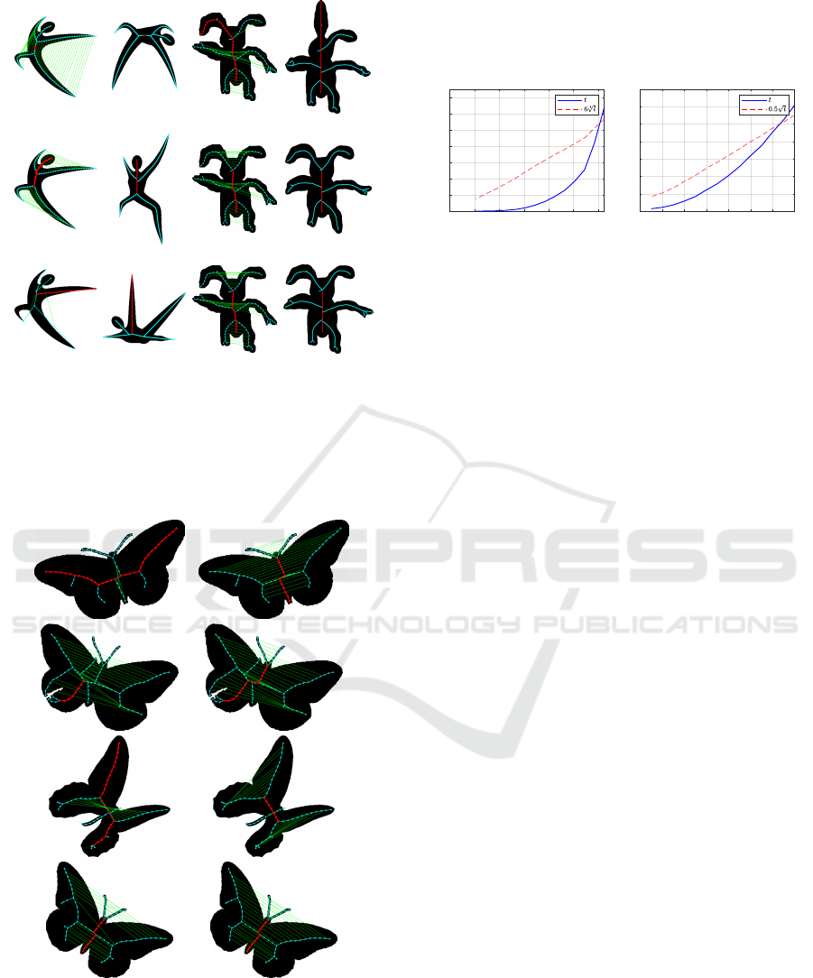
Fig. 7 shows that the proposed method finds the
symmetry axis which is either similar to or better
than provided by the alternative method. An advan-
tage of the proposed method is the highly efficient
image straightening procedure which can straighten
fragments of the share separately from the symmetry
axis. The results are better both aesthetically and in
terms of the Jaccard index: in most cases, it is higher
for straightened images. Note that the correlation of
the Jaccard index J and its approximation
˜
J for this
set is 0.8165.
Let us discuss the reasons for the method failure
with these images. Fig. 8ab shows the effects of the
area characteristics of the skeleton edges. In terms of
the Jaccard index, it is more favorable to compare the
shape fragments that are close in size (top row) rather
than semantically identical (middle row). If we ignore
the area and consider all branches of the skeleton as
individual edges, the skeleton would be symmetric in
the strict sense of graph symmetry, but the symmetry
axis again deviates from the desired one (bottom row).
The example shows that even for simple shapes, the
perception of symmetry is not purely geometric, but
involves external information.
The importance of proper selection of the pruning
parameter is shown in Fig. 8cd. In the upper row, the
ears cannot be mapped completely because the left
ear consists of several branches due to the noise (an
extra skeleton branch). The problem is solved by in-
creasing the acceptable threshold ρ of the Hausdorff
distance between the silhouettes of the original and
clipped skeletons from 3 to 4 pixels (middle row). An
alternative solution to the problem is using the exact
edge-level method. Then not only entire branches,
but their parts can be compared. A disadvantage of
this approach is the dramatic increase in the number
of edges, and decrease in performance. For this ex-
ample, the number of edges increases from 25 to 104,
and the runtime, from 8 milliseconds to 4 seconds,
i.e., by a factor of 500.
To evaluate the performance with obviously sym-
metric shapes, we used 95 images of butterflies from
the animal dataset (Bai et al., 2009) (total number of
images is 100, but 5 butterflies are shown with their
wings folded and have no symmetry). For ρ = 4,
˜
J = 0.515 J = 0.416 J = 0.329
˜
J = 0.948 J = 0.925 J = 0.425
˜
J = 0.550 J = 0.501 J = 0.470
˜
J = 0.665 J = 0.724 J = 0.478
˜
J = 0.553 J = 0.689 J = 0.598
˜
J = 0.583 J = 0.628 J = 0.724
˜
J = 0.573 J = 0.445 J = 0.501
˜
J = 0.845 J = 0.825 J = 0.445
˜
J = 0.581 J = 0.728 J = 0.643
(a) (b) (c) (d)
Figure 7: Restoration of symmetry in flexible shapes. Edge
mapping by the proposed method (a) and the (Seredin et al.,
2023) method (c). Shape straightening by the proposed
method (b) and by the alternative method (d).
l
max
= 0.05
√
W H, the symmetry axis is correctly
found in 71 images when processing branches, and
VISAPP 2025 - 20th International Conference on Computer Vision Theory and Applications
752

˜
J = 0.561 J = 0.634
˜
J = 0.570 J = 0.639
˜
J = 0.398 J = 0.413
˜
J = 0.593 J = 0.688
˜
J = 1 J = 0.377
˜
J = 0.631 J = 0.692
(a) (b) (c) (d)
Figure 8: Symmetry Restoration Errors. A shape with un-
equal areas of its mapping (a) and straightening (b) regions.
Results for various pruning parameters and the conversion
from skeleton branches to edges: mapping (c) and straight-
ening (d).
(a) (b)
Figure 9: Finding the symmetry axis: (a) at the branch level,
(b) at the edge level.
in 85 images when processing edges. Fig. 9 shows
the difference in the results. Note that
˜
J for the
edge method is guaranteed to be no lower than that
of the branch method since any correspondence be-
tween branches is representable as a correspondence
between edges.
0 20 40 60 80 100 120
0
2
4
6
8
10
12
14
0 500 1000 1500 2000 2500 3000 3500
0
0.05
0.1
0.15
0.2
0.25
0.3
0.35
(a) (b)
Figure 10: Time costs in seconds when processing (a) at the
edge level, (b) at the branch level.
The general runtime vs. number of edges E curve
is shown in Fig. 10. The experimental results agree
well with the theory. The runtime increase pat-
tern corresponds to O(|E|
4
) when comparing edges,
O(|E|
2
) when comparing branches. When using
the right exponents, the curves become linear. The
average runtime of the alternative method is 0.313
seconds, which is roughly equivalent to running a
method with 60 branches or 3500 edges.
9 CONCLUSION
We proposed a formal concept of symmetry in flex-
ible planar shapes using their skeletons. The search
for symmetry is reduced to finding the best mapping
of the original and reflected skeletons of the shape.
The optimized functional is defined in such a way as
to resemble the Jaccard area index and can be used
for its approximation. Since it consists of summands
representing the comparisons of individual edges, the
solution of the problem fits into the dynamic program-
ming paradigm. We offered an analytical solution for
distributing the shape area along the skeleton edges.
The algorithm successfully restores the symmetry of
complex flexible objects except for substantial differ-
ences in their areas (perspective distortions, for exam-
ple). In the “fast” version, the pruning parameter has
to be adjusted, while the “precise” version limits the
number of edges. Future work involves generalizing
the method to 3D shapes and, conversely, adaptation
of already existing 3D methods to the planar case.
ACKNOWLEDGEMENTS
This work was supported by the Ministry of Sci-
ence and Higher Education of the Russian Federation
Skeleton-Based Bilateral Symmetry: Theoretical Concepts and Detection via Dynamic Programming
753

within the framework of the state task FEWG-2024-
0001.
REFERENCES
Bai, X. and Latecki, L. J. (2008). Path Similarity Skele-
ton Graph Matching. IEEE Transactions on Pattern
Analysis and Machine Intelligence, 30(7):1282–1292.
Bai, X., Liu, W., and Tu, Z. (2009). Integrating contour
and skeleton for shape classification. 2009 IEEE 12th
International Conference on Computer Vision Work-
shops, ICCV Workshops, pages 360–367.
Cicconet, M., Hildebrand, D. G. C., and Elliott, H. (2017).
Finding Mirror Symmetry via Registration and Opti-
mal Symmetric Pairwise Assignment of Curves. In
2017 IEEE International Conference on Computer Vi-
sion Workshops (ICCVW), pages 1749–1758.
Huang, H., Wu, S., Cohen-Or, D., Gong, M., Zhang, H., Li,
G., and Chen, B. (2013). L1-medial skeleton of point
cloud. ACM Trans. Graph., 32(4):65:1–8.
Huang, J., Stoter, J., and Nan, L. (2023). Symmetrization of
2D Polygonal Shapes Using Mixed-Integer Program-
ming. Computer-Aided Design, 163:103572.
Jiang, W., Xu, K., Cheng, Z.-Q., and Zhang, H. (2013).
Skeleton-based intrinsic symmetry detection on point
clouds. Graphical Models, 75(4):177–188.
Kushnir, O., Fedotova, S., Seredin, O., and Karkishchenko,
A. (2017). Reflection Symmetry of Shapes Based on
Skeleton Primitive Chains. In Analysis of Images,
Social Networks and Texts, pages 293–304, Cham.
Springer International Publishing.
Li, S., Liu, X., Cao, J., and Wang, S. (2019). Organic
skeleton correspondence using part arrangements. Ap-
plied Mathematics-A Journal of Chinese Universities,
34:326–339.
Liu, J. and Liu, Y. (2011). Curved Reflection Symmetry
Detection with Self-validation. In Computer Vision
– ACCV 2010, pages 102–114, Berlin, Heidelberg.
Springer Berlin Heidelberg.
Liu, T., Kim, V., and Funkhouser, T. (2012). Finding surface
correspondences using symmetry axis curves. Com-
puter Graphics Forum, 31(5):1607–1616.
Lomov, N. and Seredin, O. (2023). Dynamic Program-
ming for Curved Reflection Symmetry Detection in
Segmented Images. The International Archives of the
Photogrammetry, Remote Sensing and Spatial Infor-
mation Sciences, XLVIII-2/W3-2023:157–163.
Mestetskiy, L. and Semenov, A. (2008). Binary Image
Skeleton – Continuous Approach. In Proceedings
of the Third International Conference on Computer
Vision Theory and Applications - Volume 1: VIS-
APP, (VISIGRAPP 2008), pages 251–258. INSTICC,
SciTePress.
Mestetskiy, L. M. and Koptelov, D. A. (2024). Constructing
the Internal Voronoi Diagram of Polygonal Figure Us-
ing the Sweepline Method. Program. Comput. Softw.,
50(4):292–303.
Nagar, R. and Raman, S. (2018). Fast and Accurate Intrinsic
Symmetry Detection. In Computer Vision – ECCV
2018, pages 433–450, Cham. Springer International
Publishing.
Qian, Z., Zhuming, H., Hui, H., Kai, X., Hao, Z., Daniel,
C.-O., and Baoquan, C. (2015). Skeleton-Intrinsic
Symmetrization of Shapes. Computer Graphics Fo-
rum, 34(2):275–286.
Seredin, O., Liakhov, D., Lomov, N., Kushnir, O., and
Kopylov, A. (2023). Greedy algorithm for fast find-
ing curvilinear symmetry of binary raster images. In
Analysis of Images, Social Networks and Texts - 11th
International Conference, AIST 2023, Yerevan, Arme-
nia, September 28-30, 2023, Revised Selected Papers,
volume 14486 of Lecture Notes in Computer Science,
pages 241–251. Springer.
Song, C., Pang, Z., Jing, X., and Xiao, C. (2018). Distance
field guided L
1
-median skeleton extraction. The Vi-
sual Computer, 34(2):243–255.
Wang, W., Ma, J., Xu, P., and Chu, Y. (2019). Intrinsic
Symmetry Detection on 3D Models with Skeleton-
guided Combination of Extrinsic Symmetries. Com-
puter Graphics Forum, 38(7):617–628.
Xu, Z. and Zhang, Q. (2016). Symmetry-Aware Human
Shape Correspondence Using Skeleton. In MultiMe-
dia Modeling, pages 632–641, Cham. Springer Inter-
national Publishing.
Yang, X., Adluru, N., Latecki, L. J., Bai, X., and Pizlo,
Z. (2008). Symmetry of Shapes Via Self-similarity.
In Advances in Visual Computing, pages 561–570,
Berlin, Heidelberg. Springer Berlin Heidelberg.
VISAPP 2025 - 20th International Conference on Computer Vision Theory and Applications
754