Construction of Football Agents by Inverse Reinforcement Learning
Using Relative Positional Information Among Players
Daiki Wakabayashi
1
, Tomoaki Yamazaki
2 a
and Kouzou Ohara
2 b
1
Graduate School of Science and Engineering, Aoyama Gakuin University, Kanagawa, Japan
2
College of Science and Engineering, Aoyama Gakuin University, Kanagawa, Japan
Keywords:
Neural Networks, Trajectory, Simulation, Multi-Agent, Reinforcement Learning.
Abstract:
Recent advancements in reinforcement learning have made it possible to develop football agents that au-
tonomously emulate the behavior of human players. However, it is still challenging for existing methods to
successfully replicate realistic player behaviors. In fact, agents exhibit behaviors like clustering around the ball
or shooting prematurely. One cause of this problem lies in reward functions that always assign large rewards
to certain actions, such as scoring a goal, regardless of the situation, which bias agents towards high-reward
actions. In this study, we incorporate the relative positional reward and the positional weight for shooting into
the reward function used for reinforcement learning. The relative positional reward, derived from the positions
of players, the ball, and the goal, is estimated using inverse reinforcement learning on a dataset of real football
games. The positional weight for shooting is similarly based on actual shooting positions observed in these
games. Through experiments on a dataset derived from real football games, we demonstrate that the relative
positional reward helps align the agents’ behaviors more closely with those of human players.
1 INTRODUCTION
With advancements in reinforcement learning tech-
niques, the development of sophisticated autonomous
agents for tasks such as self-driving and robotic con-
trol is rapidly progressing (Prudencio et al., 2024).
These autonomous agents are being applied across a
wide range of domains. In the field of sports, par-
ticularly football, numerous studies have focused on
developing football agents within simulation environ-
ments (Kitano et al., 1997; Kurach et al., 2020) us-
ing reinforcement learning to explore and analyze the
behavior of football players (Scott et al., 2021; Lin
et al., 2023; Fujii et al., 2023; Song et al., 2023a). De-
veloping football agents that closely mimic real play-
ers can offer systematic, simulation-based methods
for addressing various tasks in this domain, including
exploring diverse strategies and assessing the perfor-
mance of actual football players (Scott et al., 2021;
Song et al., 2023b).
Zhu et al. (Zhu et al., 2020) addressed the task of
controlling a single player in an 11 vs. 11 scenario. In
their study, they employed Long Short-Term Mem-
a
https://orcid.org/0009-0009-4170-725X
b
https://orcid.org/0000-0002-7399-2472
ory (LSTM) (Hochreiter and Schmidhuber, 1997)
and Proximal Policy Optimization (PPO) (Schulman
et al., 2017) to develop a football agent named We-
Kick. Lin et al. (Lin et al., 2023) proposed a dis-
tributed multi-agent reinforcement learning system
leveraging Multi-Agent Proximal Policy Optimiza-
tion (MAPPO) (Yu et al., 2022) to control 10 play-
ers, excluding the goalkeeper, in an 11 vs. 11 sce-
nario. They adopted a learning framework designed
to train agents in environments with sparse rewards.
This framework includes curriculum self-play learn-
ing, where the scenario’s difficulty is gradually in-
creased for bots with low difficulty, and challenge
self-play learning, where the agent competes against a
past version of itself that has been previously trained.
However, the football agents developed using existing
methods often struggle to replicate the movements of
real players, exhibiting behaviors such as excessively
crowding around the ball or shooting prematurely. To
address the domain gap between the actions of rein-
forcement learning-based football agents and those of
real football players, Fujii et al. (Fujii et al., 2023)
proposed a method that combines supervised learning
and reinforcement learning using a football dataset
derived from actual games. However, the resulting
agents learned only to pass the ball and shoot, with-
208
Wakabayashi, D., Yamazaki, T. and Ohara, K.
Construction of Football Agents by Inverse Reinforcement Learning Using Relative Positional Information Among Players.
DOI: 10.5220/0013322900003890
Paper published under CC license (CC BY-NC-ND 4.0)
In Proceedings of the 17th International Conference on Agents and Artificial Intelligence (ICAART 2025) - Volume 1, pages 208-217
ISBN: 978-989-758-737-5; ISSN: 2184-433X
Proceedings Copyright © 2025 by SCITEPRESS – Science and Technology Publications, Lda.

out moving toward the goal. One possible reason for
this unnatural behavior is the reward function used in
existing methods, which consistently assigns large re-
wards to certain actions, such as scoring a goal, re-
gardless of the context. This approach encourages
agents to favor specific actions with high reward val-
ues. However, it overlooks situational factors on the
pitch, such as the relative positions of players or the
number of nearby defenders, which are critical con-
siderations for decision-making in football.
In this study, we introduce a novel reward, termed
the relative positional reward, into the reward func-
tion used in reinforcement learning. The relative po-
sitional reward is derived from state features, such as
the relative distances between players, with weights
estimated from actual football games using inverse
reinforcement learning. This approach aims to en-
able the resulting agents to exhibit behaviors that
more closely resemble those of human players. Fur-
thermore, we introduce a positional weight into the
reward for shooting. This weight is based on the
distribution of shooting positions observed in actual
matches, assigning larger values to areas where real
players are more likely to take shots. This weight
helps suppress unnatural shooting from unrealistic
positions. In the experimental evaluation, we demon-
strate the effectiveness of the proposed method in
training agents to exhibit behaviors that closely re-
semble those of real players. Specifically, we ana-
lyze the distance between the positional distributions
of football agents trained on actual football datasets
and those of real players, as well as the distance be-
tween their action distributions.
2 RELATED WORK
Reinforcement learning is a framework of machine
learning where an agent learns to perform specific
tasks through interactions with its environment. In
this process, the agent observes the current state of
the environment and determines its actions accord-
ingly. The actions the agent takes cause a transition
in the state, and based on the new state, the agent re-
ceives a reward from the environment. By repeating
this process, the agent learns a policy, i.e., a strategy
for action, that maximizes the cumulative reward. Q-
learning (Watkins and Dayan, 1992) is a fundamen-
tal reinforcement learning method that learns a policy
based on the Q-value, which represents the value of
taking action a in state s. It repeatedly updates the
action-value function Q(s, a), which predicts the Q-
value. In contrast, Deep Q Network (DQN) (Watkins
and Dayan, 1992) is a deep reinforcement learning
algorithm that uses a neural network to approximate
the action-value function in Q-learning. The neu-
ral network that approximates this action-value func-
tion is referred to as the Q Network. In DQN, the
same action-value function is used for both select-
ing actions and evaluating them, which introduces
noise into the estimation process and often results in
overestimated action-values. To address this, Has-
selt et al. (Van Hasselt et al., 2016) proposed Dou-
ble Deep Q-Network (DDQN), which separates the
action-value function used for action selection from
the one used for evaluation, effectively reducing noise
and mitigating overestimation.
In the domain of building football agents, Zhu
et al. (Zhu et al., 2020) tackle the task of control-
ling a single player at all times in an 11 vs. 11
scenario within the Google Research Football (GRF)
environment, which is a 3D football simulation en-
vironment designed for reinforcement learning. In
the GRF environment, agents learn to dribble, shoot,
and pass through interactions, ultimately mastering
the skills necessary to score goals. They developed
a football agent called WeKick, using Long Short-
Term Memory (LSTM) and Proximal Policy Opti-
mization (PPO), which is one of actor-critic reinforce-
ment learning methods. Wang et al. (Wang et al.,
2022) addressed the challenge of sparse rewards in
a 5 vs. 5 multi-agent scenario by proposing a method
where agents learn two distinct policies: one driven
by individual rewards for actions such as shooting
and passing, and another based on team rewards for
achieving goals. Their approach incorporates the sim-
ilarity of action selection probabilities between the
two policies into the loss function. Li et al. (Li et al.,
2021) proposed a loss function that maximizes the
mutual information between the trajectories of agents
in a 3 vs. 1 scenario to promote diversity in agent be-
havior. This approach encourages agents to explore
extensively and select diverse actions. As a result,
during offensive plays, off-ball agents began choos-
ing actions that effectively draw defenders away.
On the other hand, in a multi-agent environment
scenario controlling 10 players (excluding the goal-
keeper) in an 11 vs. 11 game, Lin et al. (Lin et al.,
2023) proposed a distributed multi-agent reinforce-
ment learning system using Multi-Agent Proximal
Policy Optimization (MAPPO) (Yu et al., 2022). To
train agents in environments with sparse rewards, they
introduced a learning framework incorporating two
strategies: curriculum self-play and challenge self-
play. Curriculum self-play gradually increases the
scenario difficulty against lower-skilled bots, whereas
challenge self-play involves agents competing against
earlier trained versions of themselves. In evaluation
Construction of Football Agents by Inverse Reinforcement Learning Using Relative Positional Information Among Players
209

experiments, their football agents demonstrated su-
perior performance compared to existing agents in
both win rate and goal differential. Similarly, Song
et al. (Song et al., 2023a) developed a highly capable
football agent through self-play learning. While these
football agents are designed to achieve a high win
rate against rule-based bots or reinforcement learning
agents, they still face challenges in closely replicating
the movements of real players.
Unlike these studies, some research focuses on
building agents with more realistic movements by
utilizing trajectory data derived from real players.
Huang et al. (Huang et al., 2021) proposed an of-
fline reinforcement learning approach, leveraging pre-
training demonstration data from the behavioral data
of the WeKick football agent, which includes states,
actions, and rewards. In this framework, actions with
higher rewards in the demonstration data are assigned
greater weight to ensure they are prioritized during
training. As a result, their method achieved the high-
est win rate compared to existing football agents in an
11 vs. 11 scenario. Additionally, they demonstrated
that their approach improves the learning speed of
multi-agent reinforcement learning.
Fujii et al. (Fujii et al., 2023) proposed a learn-
ing method combining a pre-trained action classifier
and reinforcement learning to bridge the domain gap
between football agents and real players. The clas-
sifier, trained on a football dataset derived from real
matches, predicts player actions for given states. Us-
ing DDQN, they trained the agent by sampling actions
in the reinforcement learning environment with the
pre-trained model and integrating these samples with
demonstration data stored in a buffer. As a result, their
football agents achieved higher accuracy compared to
existing ones in terms of reward acquisition and tra-
jectory similarity to demonstration data, measured us-
ing the DTW distance (Vintsyuk, 1968). However,
the agents failed to exhibit realistic behavior, as they
learned only to pass and shoot the ball without mov-
ing toward the goal. This unnatural behavior can be
attributed to the fixed nature of the reward function,
where rewards for events like goals and shots are al-
ways the same regardless of the situation. Such a rigid
reward structure tends to bias the agent toward spe-
cific high-reward actions, while neglecting contextual
factors essential for decision-making in football, such
as player positioning and the number of surrounding
defenders.
3 PROPOSED METHOD
3.1 Overview
This study aims to develop football agents that ex-
hibit behaviors closer to those of real football play-
ers. To this end, we introduce a novel reward, re-
ferred to as the Relative Positional Reward, into the
reward function of a reinforcement learning frame-
work. This reward is calculated based on the values
of state features and adjusts the basic reward for an
agent’s actions by either enhancing or discounting it,
depending on the positional relationships between the
target agent and other entities, such as other agents,
the ball, and the goal. In the proposed method, in-
verse reinforcement learning is applied to demonstra-
tion data obtained from real football matches to es-
timate the weights for the state features used in cal-
culating the Relative Positional Reward. In ordinary
reinforcement learning, the goal is to learn a policy
that selects appropriate actions in each state based on
rewards provided by the environment. In contrast, in-
verse reinforcement learning optimizes a reward func-
tion to enable learning the correct policy by using the
actions of experts as a reference. The overview of the
proposed method is illustrated in Figure 1.
As illustrated in Figure 1, the proposed method
comprises three steps: preprocessing, inverse rein-
forcement learning, and reinforcement learning. In
the preprocessing step, the demonstration data is
constructed using tracking data from real football
matches. Specifically, we derive sequences of con-
secutive actions from the real tracking data. The state
at each time-step in a sequence is described with state
features. We adopt two types of state features: global
state features and relative state features. The global
state features represent the overall environment, such
as the positional coordinates of all players. In con-
trast, the relative state features, which are based on
each player, describe the relative relationships from
the perspective of that player, such as the distances
between the target player and other players. For the
relative state features, we further calculate their ex-
pectations for player k, µ
µ
µ
E,k
. In the inverse reinforce-
ment learning step, the weights of the relative state
features, w
w
w
k
, used to compute the Relative Positional
Reward R
∗
k
are optimized to minimize the difference
between the expected values of the relative state fea-
tures for a real player (expert) k, µ
µ
µ
E,k
, and those of its
corresponding agent under policy π
k
,
¯
µ
µ
µ
E,k
(π
k
). In the
final reinforcement learning step, each football agent
k is trained to behave similarly to a real football player
by learning the policy π
′
k
. This training uses a total
reward function composed of the sum of the Relative
ICAART 2025 - 17th International Conference on Agents and Artificial Intelligence
210

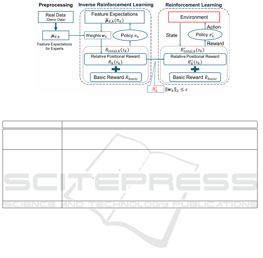
Figure 1: Overview of the proposed method for developing an agent that corresponds to expert player k, wherer s
k
represents
a state associated with player k.
Table 1: Relative state features with respect to agent a.
Type State Features (notation)
Distance
distance to the n-th closest offensive player (D
off
n
(a)), distance to the n-th
closest defensive player (D
def
n
(a)), distance to a keeper (D
keeper
(a)), distance
to the ball, distance to the goal (D
goal
(a))
Proportion of players
in a specific area
proportion of offensive players within a radius r (P
off
r
(a)), proportion of de-
fensive players within a radius r (P
def
r
(a)). proportion of offensive players up
to the goal line (P
off
goal line
(a)), proportion of defensive players up to the goal
line (P
def
goal line
(a)), proportion of offensive players up to the goal (P
off
goal
(a)),
proportion of defensive players up to the goal (P
def
goal
(a)), proportion of of-
fensive players unobstructed by defenders on a direct line from the agent a
(P
off
(a)), proportion of defenders on the direct line to the ball (P
def
ball
(a))
Angle angle to the goal (A(a))
Positional Reward R
∗
k
and a basic reward R
basic
, which
is a discrete reward for specific events commonly em-
ployed in existing research.
3.2 Status Features
As mentioned above, each state comprising an ac-
tion sequence is described using relative state fea-
tures, alongside the global state features commonly
employed in the literature. The positional coordi-
nates of players and the ball are typical examples of
global state features. In contrast, relative state fea-
tures are based on a specific player or agent. For ex-
ample, these features include the distances between
the player/agent and other players/agents. Table 1
provides the complete list of relative state features
used in this study.
Among these features, the distance between play-
ers is modeled by considering the distribution of rel-
ative distances observed in real game play. Specif-
ically, instead of the actual distance between players
x
α
n
, the value of the following Gaussian function f (x
α
n
)
is used as one of the relative state features:
f (x
α
n
) = e
−(3x
α
n
−d
α
n
)
2
, (1)
where α is an index that indicates whether the dis-
tance refers to that to an offensive player, a defensive
player, or the goalkeeper. Accordingly, the value x
α
n
represents the distance from the observed player or
agent to the n-th closest agent of type α. Meanwhile,
d
α
n
denotes the average distance to the n-th closest
player, derived from real data. The value of f (x
α
n
)
increases as x
α
n
gets closer to d
α
n
.
3.3 Preprocessing Real Tracking Data
In the preprocessing step, action sequences are ex-
tracted from real tracking data (demonstration data),
and the state at each time step is represented using the
previously described state features. The global state
features are defined for each state, while the relative
state features are specified for each player within a
state. We further calculate the expected values of rel-
ative status features for a player k, µ
µ
µ
E,k
, which are
Construction of Football Agents by Inverse Reinforcement Learning Using Relative Positional Information Among Players
211

used as the expert’s values in inverse reinforcement
learning. µ
µ
µ
E,k
is a vector defined as follows:
µ
µ
µ
E,k
=
1
m
m
∑
i=1
∞
∑
t=0
γ
t
φ
φ
φ(s
(i)
t,k
), (2)
where s
(i)
t,k
is the i-th state transition sequence of length
m for player k in the demonstration data, and φ
φ
φ(·) is
a function that transforms the state s
t
into a vector
representing the values of the relative state features.
Namely, φ
φ
φ(s
(i)
t,k
) represents the relative state features
for the state s
(i)
t,k
.
3.4 Reward Function
The reward function in the proposed method consists
of the basic reward function, which is commonly used
in existing research, and the Relative Positional Re-
ward newly introduced in this study. The basic reward
R
basic
is defined as follows:
R
basic
= w
shot
∗ R
shot
+ R
goal
+ R
conceded
+ R
gain
+ R
lost
+ R
receive
+ R
block
+ R
o f f side
(3)
where R
shot
, R
goal
, R
conceded
, R
gain
, R
lost
, R
receive
,
R
block
, and R
o f f side
are the reward values given for
shooting, scoring a goal, conceding a goal, winning
the ball, losing the ball, receiving a pass, blocking,
and being offside, respectively. The shot reward R
shot
is a reward directly assigned to a shooting action.
This encourages the agent to recognize shooting as
the most effective action for scoring a goal, which
carries a high reward value. To mitigate this bias
toward shooting, we divided the football half-court
into a grid and applied the position-specific shot rate
w
shot
, derived from actual data, as a weight for the
shot reward. This method is expected to discourage
the agent from learning behaviors that involve taking
forced shots from positions far from the goal. The
basic reward is assigned exclusively to the relevant
player, whereas the offside reward is distributed to the
entire team. Additionally, the basic reward is utilized
in both the inverse reinforcement learning and rein-
forcement learning processes. On the other hand, the
relative positional reward R
k
(s
k
) of the agent k is de-
fined as follows:
R
k
(s
k
) = w
w
w
k
· φ
φ
φ(s
k
), (4)
where w
w
w
k
is a weight vector associated with the state
s
k
, which is represented by the relative state features.
3.5 Learning Relative Positional
Reward with Inverse Reinforcement
Learning
In inverse reinforcement learning, the weight vec-
tor w
w
w
k
is optimized. Specifically, the relative posi-
tional reward R
k
(s
k
) is estimated together with the ba-
sic reward R
basic
, considering the total reward func-
tion R
total,k
(s
k
) in the reinforcement learning per-
formed within the inverse reinforcement learning
step. R
total,k
(s
k
) is defined as follows:
R
total,k
(s
k
) = R
basic
+ R
k
(s
k
) (5)
When the expert’s feature expectation value µ
µ
µ
E,k
is
given, the weights w
w
w
k
are determined in such a way
as to minimize the error between the expert’s feature
expectation value
¯
µ
µ
µ
E,k
(π
k
) and the expert’s feature ex-
pectation value µ
µ
µ
E,k
under the policy π
k
, which obeys
the reward function R
total,k
(s
k
). Here, the observed
feature expectation value,
¯
µ
µ
µ
E,k
(π
k
), is defined as in
Equation (6).
¯
µ
µ
µ
E,k
(π
k
) = E[
∞
∑
t=0
γ
t
φ
φ
φ(s
k
)|π
k
], (6)
where γ is the discount factor in reinforcement learn-
ing. In this study, we use the Projection-based
Method (PM), an inverse reinforcement learning
method proposed by Abbeel and Ng (Abbeel and Ng,
2004), to estimate the weight w
w
w
k
.
3.6 Learning Behaviors with
Reinforcement Learning
During reinforcement learning, the policy π
′
k
is
learned using the estimated relative positional reward
R
∗
k
(s
k
) and the basic reward R
basic
defined by Equa-
tion (3) as the reward function for the football agent.
The reward function R
∗
total,k
(s
k
) used in reinforcement
learning is expressed by Equation (7).
R
∗
total,k
(s
k
) = R
basic
+ R
∗
k
(s
k
) (7)
4 EXPERIMENTAL EVALUATION
4.1 Experimental Setup
4.1.1 Learning Environment
In this study, we used Google Research Football
(GRF) (Kurach et al., 2020) as the football simula-
tion environment. GRF is a reinforcement learning
environment for learning football movements, and the
ICAART 2025 - 17th International Conference on Agents and Artificial Intelligence
212

agent learns how to score goals such as passing and
shooting through interaction with the environment.
The size of the pitch is in the range −1 to +1 on
the x axis and −0.42 to +0.42 on the y axis, and the
size of the goal is in the range −0.044 to +0.044 on
the y axis. In this study, we only experimented with
the offense in order to simplify the experiment, and
conducted experiments with a scenario of four offen-
sive players and eight defensive players. For the de-
fense, we used a bot that follows the ball and moves
to its own team using a rule-based approach provided
by GRF. The initial positions of the agents in each
episode were set to the positions of all the players
when they received an assist pass in the shooting se-
quence of the real data. The actions taken by the
agents were limited to 12 types: moving in 8 direc-
tions in 45-degree increments, doing nothing, high
pass, short pass, and shoot. The states observed by
the agents were 44-dimensional (the x and y coordi-
nates for each player, the position coordinates of the
ball, a one-hot vector of 3 dimensions for the team
holding the ball (left team, right team, and non-ball-
holding state), and a one-hot vector of 11 dimensions
for the player IDs (11 players per team), for a total of
61-dimensional vectors. The episode ended when the
conditions for switching between offense and defense
were met, such as when a goal was scored, a goal was
conceded, or the ball was lost, or when 100 steps had
elapsed. For the weight of the shoot reward, we di-
vided the half court of football into five parts on the
x axis and eight parts on the y axis, and used the per-
centage of shots by position in the goal sequence of
the actual data calculated for each grid.
4.1.2 Dataset
In this study, we used event data and tracking data
from 95 J1 League games in 2021 and 2022 provided
by the 2023 Sports Data Science Competition. From
this dataset, we extracted 1,520 sequences from the
time an assist pass was made to the time a shot was
taken, and divided them into 141 goal sequences and
1,379 shot sequences. As a preprocessing step, we ex-
tracted only sequences in which there were 22 players
and a ball on the court, and downsampled them from
25 Hz to 8.33 Hz. We used these sequences for in-
verse reinforcement learning (proposed method), pre-
training (comparison method (Fujii et al., 2023)), and
reinforcement learning. For inverse reinforcement
learning (proposed method) and pre-training (com-
parison method), the data was divided into 102 train-
ing sequences and 39 validation sequences for the
goal sequence. For reinforcement learning, the ini-
tial position data for the shoot sequence was divided
into 1,179 training initial positions and 100 test initial
positions for the positions of all players when they
receive an assist pass. In addition, 100 shooting se-
quences were used as the teacher data to be stored in
the buffer during reinforcement learning in the com-
parative method. The four offensive players selected
as the experimental subjects were the players who
made the assist pass, the player who took the shot,
and two other players who were close to the goal but
not the two players mentioned above. The eight de-
fensive players were seven players close to the goal
and the goalkeeper.
4.1.3 Learning Parameters
We implemented the proposed method using DDQN
for the reinforcement learning component and DQN
for the inverse reinforcement learning component.
This method, referred to as DDQ IRL, was then com-
pared with both DDQN and DQAAS (Fujii et al.,
2023). Table 2 shows the basic learning parameters
for DQN and DDQN, such as batch size and dis-
count rate. We set common values for these param-
eters in both methods. Additionally, the number of
update steps for the Q-Network, a parameter specific
to DDQN, was set to 10, 000. Moreover, we used Pri-
oritized Experience Replay as a sampling method for
experience data from the buffer, as in Fujii et al. (Fu-
jii et al., 2023). In the loss function of DQAAS, λ
1
,
the weight for the supervised learning term, was set
to 0.04, while λ
2
, the weight for the regularization
term, was set to 1.00. The convergence threshold for
inverse reinforcement learning in DDQN IRL, ε, was
set to 0.1. In addition, for the parameters of the state
feature, we used four different values for r, the ra-
dius used to calculate the proportion of people: 0.1,
0.2, 0.3, and 0.4. For d
α
n
in Equation (1), which rep-
resents the distance to the n-th closest offense or de-
fense player, or the distance to the keeper, we adopted
the following values: in ascending order of relative
distance, 0.16, 0.25, and 0.36 for offense; 0.08, 0.13,
0.16, 0.21, 0.24, 0.28, 0.33, and 0.44 for defense; and
0.35 for the keeper. Note that α denotes either “of-
fense,” “defense,” or “keeper.”
4.1.4 Evaluation Metrics
In this study, we used the Kullback-Leibler (KL) di-
vergence (Yeh et al., 2019) shown in Equation (8) as
an evaluation metric to evaluate the distance between
the position distribution and the action distribution of
the learned football agent and the real player.
KL(P ∥ Q) =
∑
x
P(x)log
P(x)
Q(x)
(8)
Here, P(x) represents the distribution of players in
the real data, and Q(x) represents the distribution of
Construction of Football Agents by Inverse Reinforcement Learning Using Relative Positional Information Among Players
213

Table 2: Settings for the basic parameters of DQN and
DDQN.
Parameter Value
Batch size 500
Intermediate layer size 256
Discount rate 0.99
Learning Rate 0.00025
Optimizer Adam
n step 16
Warm-up samples 2,000
Initial terminate condition ε 1.00
Last terminate condition ε 0.02
ε decay step 10,000
Table 3: The distance between the position distributions of
the agents in each model and real players.
offensive agents
Model all on-ball off-ball
DQAAS 0.095 0.273 0.174
DDQN 0.158 0.444 0.167
DDQN IRL 0
0
0.
.
.0
0
06
6
60
0
0 0
0
0.
.
.2
2
20
0
05
5
5 0
0
0.
.
.0
0
08
8
81
1
1
the learned agent. In addition, in the evaluation of
the position distribution distance, x represents each
grid when the football half-court is divided into grids,
and in the evaluation of the action distribution dis-
tance, x represents the action. Using these metrics,
we compared our proposed method, DDQN IRL with
the method proposed by Fujii et al. (Fujii et al., 2023),
DQAAS, and DDQN.
4.2 Results and Discussion
The position distribution distances and action distri-
bution distances of the agents of each model and the
real players are shown in Tables 3 and 4 respectively.
From Table 3, we can see that the football agents us-
ing the proposed method have the position distribu-
tions closest to those of the real players in all items for
the entire offense, on-ball agents, and off-ball agents,
compared to DQAAS and DDQN. From Table 4, we
can see that the proposed method’s agents have the
action distribution closest to that of real players. This
shows that the relative positional reward introduced in
the proposed method contributes to making the posi-
tion distribution and action distribution of the football
agents after learning closer to that of real players.
In this section, we analyzed the agents in each
model by dividing them into on-ball agents and off-
ball agents. Here, to check whether the on-ball agents
shoot near the goal like real players, we examined the
distance between the on-ball agent’s shooting posi-
tion and the goal. The results are shown in Table 5. In
order to maintain fairness in the comparison, only se-
quences in which the agents of each model shoot the
Table 4: The distance between the action distributions of
the agents in each model and real players.
offensive agents
Model all on-ball off-ball
DQAAS 9.950 10.20 10.800
DDQN 0.406 5.10 0.440
DDQN IRL 0
0
0.
.
.2
2
26
6
62
2
2 2
2
2.
.
.6
6
64
4
4 0
0
0.
.
.3
3
34
4
44
4
4
Table 5: The average distance from the shooting position to
the goal.
Model Average distance
Real players 0.245
DQAAS 0.289
DDQN 0.255
DDQN IRL 0.221
ball were extracted. In this case, the average distance
from the initial position of the agent to the goal is
0.270. From this result, it can be seen that the agents
in the proposed method tend to shoot the ball from the
position closest to the goal. In addition, it can be seen
that DQAAS tends to shoot from a position further
away than the initial position, and that DDQN tends
to shoot from a position slightly further away than the
real player. Next, we show some trajectories of the
real players and the on-ball agents of each model until
they shoot the ball in Figures 2a and 2d . In these di-
agrams, the initial position of the agent is represented
by a red dot, the movement trajectory by a blue line,
the shooting position by a yellow star mark, and the
passing position by a yellow square. From Figure 2b,
we can see that the comparative method DQAAS has
a strong tendency to choose a path. On the other hand,
from Figures 2c and Figure 2d, it can be seen that the
proposed method, compared to DDQN, moves closer
to the goal before shooting, as in the case of a real
player (Figure 2a), even when the initial position is
far from the goal. From this, we can see that rela-
tive positional reward can contribute to the learning
of shooting actions in positions close to the on-ball
agent’s goal.
Here, the weights of the reward function estimated
by inverse reinforcement learning are shown in Ta-
ble 6. Agent 1 represents the on-ball agent, and agents
0, 2, and 3 represent the off-ball agents. By observing
the individual weights, we can see that the weights
for the distance features of the on-ball agent with the
keeper are positive. In addition, the weights for the
distance to the goal and the percentage of defend-
ers within the goal line have negative weights, and
the absolute values of these weights are larger than
the weights for similar state features of the off-ball
agents. These weights may contribute to the learning
ICAART 2025 - 17th International Conference on Agents and Artificial Intelligence
214

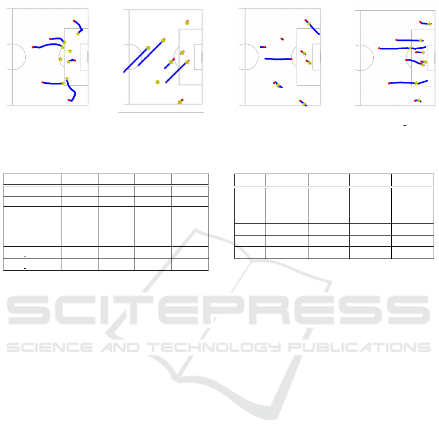
(a) Real players. (b) DQAAS. (c) DDQN. (d) DDQN IRL.
Figure 2: The trajectory leading to the shot for agents trained with each method.
Table 6: The weights of the reward function of on-ball
agents.
agent
off
0
agent
on
1
agent
off
2
agent
off
3
D
keeper
0.041 0.061 0.020 0.039
D
goal
−0.010 −0.058 −0.022 −0.043
P
def
r
(r = 0.1) 0.024 −0.019 0.016 0.007
(r = 0.2) 0.022 −0.015 −0.002 −0.010
(r = 0.3) −0.008 −0.005 −0.000 −0.062
(r = 0.4) −0.009 −0.066 −0.007 −0.056
P
def
goal line
−0.009 −0.066 −0.007 −0.056
P
def
goal line
−0.017 −0.023 −0.023 −0.002
of shooting behavior in positions close to the goal for
on-ball agents. In addition, negative weights are also
given to the weights for the percentage of defenders
within a radius r and the percentage of defenders up
to the goal, and in particular, the weight for the per-
centage of defenders up to the goal is −0.066, and the
absolute value of the weight is large compared to the
weight of the off-ball agent. This weight is thought to
represent the characteristics of the on-ball player who
is aiming to shoot.
Next, we checked whether the relative distances
taken by the off-ball and on-ball agents were close to
the distribution of the relative distances taken by real
players. The relative distances between the off-ball
and on-ball agents of Agent 2 in the test sequences
(100 cases) are shown in Figures 3a and 3d . In or-
der to unify the verification environment, the on-ball
agent and the defense agent were made to move in the
same way as real players. As a result, from Figure 3d,
we can see that the relative distance taken by the off-
ball and on-ball agents of the proposed method is
close to the distribution of the relative distance taken
by the off-ball and on-ball players in real players (Fig-
ure 3a). Similarly, from Figure 3b, we can see that
DQAAS also has a distribution of relative distances
that is close to that of real players. On the other hand,
from Figure 3c, we can see that the relative distance
of DDQN tends to increase with each step. From this,
we can see that relative positional reward may con-
tribute to the off-ball agent learning movements that
Table 7: The weights of the reward function for off-ball
agents.
agent
off
0
agent
on
1
agent
off
2
agent
off
3
D
off
1
−0.004 −0.025 −0.007 −0.005
D
off
2
0.004 0.015 0.002 0.002
D
off
3
0.019 0.005 0.002 0.001
D
ball
−0.004 0.011 −0.029 −0.013
D
goal
−0.010 −0.058 −0.022 −0.043
P
def
ball
0.007 0.020 −0.022 0.010
approach the distribution of the relative distance in re-
ality. As shown in Figures 4 and 5, a similar trend can
be seen for other agents.
Here, the weights of the reward function estimated
by inverse reinforcement learning are shown in Ta-
ble 7. From Table 7, we can see that the weights
for the distance features of the off-ball agent’s clos-
est offense are all negative, but the absolute value is
smaller than the weight of −0.025 given to the sim-
ilar state features of the on-ball agent. Therefore, it
is possible to say that the weights attached to the dis-
tance features contribute to the off-ball agent learning
movements that make the relative distance between
the on-ball agent and the off-ball agent closer to the
distribution of the relative distance in reality. In ad-
dition, the weights for the distance to the ball and the
distance to the goal for the off-ball agents are all neg-
ative, meaning that the weights are such that the off-
ball agents learn to behave in a way that brings them
closer to the on-ball agents and the goal. On the other
hand, the weights for the percentage of defenders on
a straight line to the ball are positive for Agents 0 and
3, at 0.007 and 0.010 respectively. As one of the roles
of an off-ball player is to receive passes from on-ball
players, it is desirable that the weight here is negative
rather than positive.
Construction of Football Agents by Inverse Reinforcement Learning Using Relative Positional Information Among Players
215

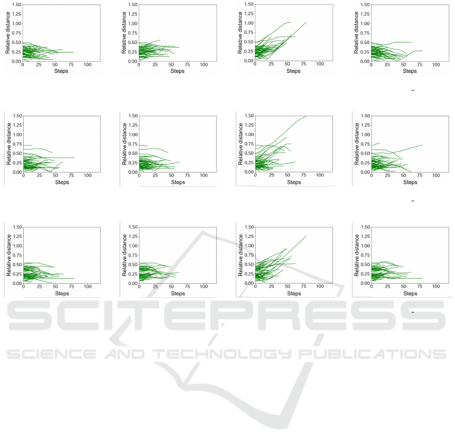
(a) Real players. (b) DQAAS. (c) DDQN. (d) DDQN IRL.
Figure 3: The relative distance between the on-ball player/agent and the off-ball player/agent 2.
(a) Real players. (b) DQAAS. (c) DDQN. (d) DDQN IRL.
Figure 4: The relative distance between the on-ball player/agent and the off-ball player/agent 0.
(a) Real players. (b) DQAAS. (c) DDQN. (d) DDQN IRL.
Figure 5: The relative distance between the on-ball player/agent and the off-ball player/agent 3.
5 CONCLUSION
This study proposes a method to develop a football
agent mimicking real players by estimating player-
centric relative rewards from actual football data us-
ing inverse reinforcement learning and applying them
as reward functions in reinforcement learning. We
also demonstrated the effectiveness of the proposed
method quantitatively and qualitatively through the
experiments using real football data. For future work,
we plan to establish a correlation between the basic
reward function and the state reward function. In the
proposed method, the state reward function is inde-
pendently learned from the basic reward function us-
ing inverse reinforcement learning. However, as ac-
tions like shooting or passing depend on the current
state, it is essential to design the reward function so
that the state influences the rewards for these actions
and to learn the extent of this influence. Additionally,
the adversarial learning strategy used in this study
needs refinement to ensure the resulting agents’ be-
haviors are more stable.
ACKNOWLEDGEMENTS
This work was partly supported by a grant from
the Center for Advanced Information technology Re-
search, Aoyama Gakuin University.
REFERENCES
Abbeel, P. and Ng, A. Y. (2004). Apprenticeship learning
via inverse reinforcement learning. In Proceedings of
the 21th International Conference on Machine learn-
ing (ICML 2004).
Fujii, K., Tsutsui, K., Scott, A., Nakahara, H., Takeishi, N.,
and Kawahara, Y. (2023). Adaptive action supervision
in reinforcement learning from real-world multi-agent
demonstrations. arXiv preprint arXiv:2305.13030.
Hochreiter, S. and Schmidhuber, J. (1997). Long short term
memory. Neural Computation, 9(8):1735–1780.
Huang, S., Chen, W., Zhang, L., Xu, S., Li, Z., Zhu,
F., Ye, D., Chen, T., and Zhu, J. (2021). Ti-
kick: Towards playing multi-agent football full games
from single-agent demonstrations. arXiv preprint
arXiv:2110.04507.
Kitano, H., Asada, M., Kuniyoshi, Y., Noda, I., and Osawa,
E. (1997). The robot world cup initiative. In Pro-
ICAART 2025 - 17th International Conference on Agents and Artificial Intelligence
216

ceedings of the 1st International Conference on Au-
tonomous agents (AGENTS 1997), pages 340–347.
Kurach, K., Raichuk, A., Stanczyk, P., Zajac, M., Bachem,
O., Espeholt, L., Riquelme, C., Vincent, D., Michal-
ski, M., Bousquet, O., and Gelly, S. (2020). Google
research football: A novel reinforcement learning en-
vironment. In Proceedings of the 34th AAAI Con-
ference on Artificial Intelligence (AAAI 2020), vol-
ume 34, pages 4501–4510.
Li, C., Wang, T., Wu, C., Zhao, Q., Yang, J., and Zhang, C.
(2021). Celebrating diversity in shared multi-agent re-
inforcement learning. In Advances in Neural Informa-
tion Processing Systems (NeurIPS 2021), pages 3991–
4002.
Lin, F., Huang, S., Pearce, T., Chen, W., and Tu, W.-W.
(2023). Tizero: Mastering multi-agent football with
curriculum learning and self-play. In Proceedings
of the 2023 International Conference on Autonomous
Agents and Multiagent Systems (AAMAS 2023), pages
67–76.
Prudencio, R. F., Maximo, M. R. O. A., and Colombini,
E. L. (2024). A survey on offline reinforcement learn-
ing: Taxonomy, review, and open problems. IEEE
Transactions on Neural Networks and Learning Sys-
tems, 35(8):10237–10257.
Schulman, J., Wolski, F., Dhariwal, P., Radford, A., and
Klimov, O. (2017). Proximal policy optimization al-
gorithms. arXiv preprint arXiv:1707.06347.
Scott, A., Fujii, K., and Onishi, M. (2021). How does
ai play football? an analysis of rl and real-world
football strategies. In Proceedings of the 14th Inter-
national Conference on Agents and Artificial Intelli-
gence (ICAART 2021), volume 1, pages 42–52.
Song, Y., Jiang, H., Tian, Z., Zhang, H., Zhang, Y., Zhu,
J., Dai, Z., Zhang, W., and Wang, J. (2023a). An em-
pirical study on google research football multi-agent
scenarios. arXiv preprint arXiv:2305.09458.
Song, Y., Jiang, H., Zhang, H., Tian, Z., Zhang, W., and
Wang, J. (2023b). Boosting studies of multi-agent re-
inforcement learning on google research football envi-
ronment: the past, present, and future. arXiv preprint
arXiv:2309.12951.
Van Hasselt, H., Arthur, G., and David, S. (2016). Deep re-
inforcement learning with double q-learning. In Pro-
ceedings of 13th the AAAI conference on artificial in-
telligence (AAAI 2016), volume 30, pages 2094–2100.
Vintsyuk, T. K. (1968). Speech discrimination by dynamic
programming. Cybernetics, 4(1):52–57.
Wang, L., Zhang, Y., Hu, Y., Wang, W., Zhang, C., Gao, Y.,
Hao, J., Lv, T., and Fan, C. (2022). Individual reward
assisted multi-agent reinforcement learning. In Pro-
ceedings of the 39th International Conference on Ma-
chine Learning (PMLR 2022), pages 23417–23432.
Watkins, C. J. C. H. and Dayan, P. (1992). Q-learning. Ma-
chine learning, 8(3):279–292.
Yeh, R. A., Schwing, A. G., Huang, J., and Murphy, K.
(2019). Diverse generation for multi-agent sports
games. In Proceedings of the 2019 IEEE/CVF Con-
ference on Computer Vision and Pattern Recognition
(CVPR 2019), pages 4610–4619.
Yu, C., Velu, A., Vinitsky, E., Gao, J., Wang, Y., Bayen,
A., and Wu, Y. (2022). The surprising effectiveness
of ppo in cooperative multi-agent games. In Advances
in Neural Information Processing Systems (NeurIPS
2022), volume 35, pages 24611–24624.
Zhu, F., Li, Z., and Zhu, K. (2020). We-
kick. https://www.kaggle.com/c/google-
football/discussion/202232.
Construction of Football Agents by Inverse Reinforcement Learning Using Relative Positional Information Among Players
217