U-Net in Histological Segmentation: Comparison of the Effect of Using

Different Color Spaces and Final Activation Functions

aszl

o K

orm

oczi

and L

aszl

o G. Ny

Department of Image Processing and Computer Graphics, University of Szeged, Szeged, Hungary

{kormoczi, nyul}@inf.u-szeged.hu

Keywords:

Semantic Segmentation, U-Net, Machine Learning, Deep Learning, Color Space Conversion.

Abstract:

Deep neural networks became widespread in numerous ﬁelds of image processing, including semantic segmen-

tation. U-Net is a popular choice for semantic segmentation of microscopy images, e.g. histological sections.

In this paper, we compare the performance of a U-Net architecture in three different color spaces: the com-

monly used, perceptually uniform sRGB, the perceptually uniform but device-independent CIE L*a*b*, and

linear RGB color space that is uniform in terms of light intensity. Furthermore, we investigate the network’s

performance on data combinations that were unseen during training.

1 INTRODUCTION

Semantic segmentation of images is a key task for nu-

merous applications, including quantitative analysis

of histological sections (Chang et al., 2017; Iizuka

et al., 2020; Ahmed et al., 2022). With widespread

adoption of deep neural networks, this task is mostly

a matter of quantity and quality of the training data.

However, in several ﬁelds, such training data are lim-

ited, either in terms of quality or quantity. By the

nature of the selected task, the training dataset can

be highly imbalanced (e.g. different tissue types in

a histological section) or can differ from the data the

model is evaluated. Among other deep learning ar-

chitectures, U-Net (Ronneberger et al., 2015) became

widely adopted in the ﬁeld of semantic segmentation,

especially for biomedical images. It is a fully convo-

lutional network (ﬁrst used for segmentation by (Shel-

hamer et al., 2017)) with skip connections (introduced

in ResNet (He et al., 2016)). U-Net is popular for se-

mantic segmentation tasks due to its high generaliza-

tion ability and acceptable speed.

Images used for deep learning data (either for

training or inference) are usually stored in popular im-

age formats, like PNG that uses lossless compression,

JPEG that uses lossy compression, or TIFF, that can

use either lossy or lossless compression. These for-

mats usually use 1 (grayscale) or 3 (RGB) channels,

8 bits per channel (16 bits per channel is common for

https://orcid.org/0000-0002-3833-0609

https://orcid.org/0000-0002-3826-543X

TIFF images for scientiﬁc purposes). These image

formats use the standardized but device-dependent

sRGB color space and store intensities with lon-linear

gamma correction, to better ﬁt for human perception.

Gamma correction ensures that the intensity values

are stored in a perceptually uniform way, i.e. efﬁ-

ciently for displaying to human viewers. Contrary,

numerous image processing tasks (e.g. color blend-

ing or even resizing images) require the intensity val-

ues to be in a linear color space, i.e. uniform in terms

of physical light intensity. Image manipulation soft-

ware usually linearize the opened images for editing,

and apply gamma correction upon saving.

Another common color space is CIE L*a*b* (also

referred as CIELAB), that is perceptually based but

device independent (contrary to sRGB). It may be bet-

ter suitable for pattern recognition and semantic seg-

mentation tasks than an RGB representation, because

it separates the lightness information (L* value) from

the color information (a* and b* values).

An important question is whether a deep neural

network can beneﬁt from a perceptually uniform, de-

vice independent color space like CIE L*a*b, or a

phisically uniform, linear RGB color representation.

386

Körmöczi, L. and Nyúl, L. G.

U-Net in Histological Segmentation: Comparison of the Effect of Using Different Color Spaces and Final Activation Functions.

DOI: 10.5220/0013323300003911

Paper published under CC license (CC BY-NC-ND 4.0)

In Proceedings of the 18th International Joint Conference on Biomedical Engineering Systems and Technologies (BIOSTEC 2025) - Volume 1, pages 386-389

ISBN: 978-989-758-731-3; ISSN: 2184-4305

2 DATA

2.1 Images

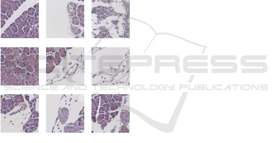
Our dataset consists of 256×256 px 3-channel 8-

bit RGB images, randomly cut from high-resolution

bright-ﬁeld optical microscopy images of pancreas

histological sections. The data is classiﬁed pixel-wise

into 3 distinct classes, i.e. background, healthy tissue

and diseased tissue. The images containing diseased

tissue are taken from histological sections with arti-

ﬁcially induced acute pancreatitis, where the whole

section is diseased. Similarly, images of healthy tis-

sue are taken from histological sections where the

whole tissue is healthy. Considering this, each sample

contains either healthy or diseased tissue, along with

background. Some of the samples can be seen in 1.

Figure 1: Sample image patches. First row: healthy, second

row: diseased, third row: mixed samples.

2.2 Training, Validation and Test

Dataset

We partition the dataset into distinct training, val-

idation and test subsets. The trainig dataset con-

tains 4500 images, with a total of 180 833184 px of

background, 25 999 369 px of normal (healthy) tis-

sue and 88 079 441 px of diseased tissue. The val-

idation dataset comprises 3016 images, with a to-

tal of 114 602 379 px of background, 20262843 px

of normal (healthy) tissue and 62 791354 px of

diseased tissue. Finally, the test set includes

3787 images, consisting of 148533175 px of back-

ground, 22 332 040 px of normal (healthy) tissue and

77319617 px of diseased tissue.

2.3 Mixed Samples

Deep neural networks generally perform well on data

similar to the training data. It is interesting though,

how they perform on data variations that were not

present during training. To evaluate the model, since

there were no samples that contained both healthy and

diseased pixels, we artiﬁcially generated mixed sam-

ples by combining samples taken from the healthy and

diseased subset of the validation dataset. Mixing was

performed using a randomly generated binary mask

that contained 5 potentially overlapping ellipsoids of

random size, orientation and location. The masks

were blurred and then thresholded, to have a more

natural appearance in the corners resulting from over-

lapping ellipsoids. The new image sample is gener-

ated by taking parts from a diseased sample where the

mask is 0 and from a healthy sample where the mask

is 1. These new images may contain both healthy and

diseased tissue, along with background.

This new mixed dataset consists of 1497 im-

ages, with a total of 52876272 px of back-

ground, 7 895 774 px of normal (healthy) tissue and

37335346 px of diseased tissue.

3 ARCHITECTURE

Using U-Net for semantic segmentation is popular

and well-documented (Du et al., 2020). We used a

U-Net architecture of 5 encoder-decoder block pairs,

with 1 px padding at the convolutional layers to keep

original image dimensions at the output segmentation.

Although softmax is the preferred activation function

when having mutually exclusive classes in a semantic

segmentation task, we also trained the model using

sigmoid instead of softmax and examined the differ-

ences.

4 TRAINING THE MODEL

The images of our dataset were originally stored in

3-channel PNG image format, in sRGB color space,

gamma-encoded. For comparison of the effect of the

color space (i.e. gamma-encoded sRGB, linear RGB

and CIE L*a*b*), we trained and evaluated different

models of the same architecture (described in Section

3), with both the training and validation dataset con-

verted to the 3 different color spaces. Furthermore,

to investigate the effect of changing the activation

function of the output layer, we trained a model with

U-Net in Histological Segmentation: Comparison of the Effect of Using Different Color Spaces and Final Activation Functions

387

softmax and another with sigmoid on all three color

spaces, so as a result, we have 6 models to compare.

For training the models, we used Adam optimizer

with an initial learning rate of 0.001 and a learning

rate scheduler was utilized for better convergence.

We used Categorical Cross-Entropy loss, weighted to

compensate for the imbalanced dataset. The training

was run for 160 epochs, with a batch size of 8. Train-

ing was performed on a desktop computer, having an

NVIDIA RTX 3060 Ti GPU with 8GB VRAM.

5 RESULTS

5.1 Evaluation Metrics

We evaluated the 6 different models on both the orig-

inal validation dataset and on the generated, artiﬁ-

cially mixed images. For performance metrics, we

used confusion matrix, per-class precision, recall, F1

score and micro-averaged F1 score, that equals to

micro-averaged precision and micro-averaged recall.

While per-class metrics are sensitive to class imbal-

ance, micro-averaged F1 score is implicitly compen-

sated for that effect and gives an impression on the

overall performance of the model. This note is im-

portant, because one of the 3 classes (healthy tis-

sue) has weak support in the mixed dataset (8 million

pixels compared to 53 million pixels background and

37 million pixels diseased tissue), as detailed in Sec-

tion 2.3.

For each trained model, regardless of the ﬁnal ac-

tivation function used in that model, we considered

the class with the highest predicted probability for a

pixel as the predicted class for that pixel.

The confusion matrix provides detailed informa-

tion for each class, including the number of data sam-

ples (pixels, in this case) that were correctly predicted

as that class (true positives, denoted as T P), as well

as those misclassiﬁed as other classes. This includes

false positives (samples incorrectly predicted as the

given class, denoted as FP) and false negatives (sam-

ples from the given class incorrectly predicted as an-

other class, denoted as FN).

Precision is the ratio of true positives and all pre-

dictions for a given class, while recall is the ratio of

true positives and all pixels originally labeled as the

given class. F1 score is calculated as

= 2 ×

precision

× recall

precision

+ recall

for the ith class.

Micro-averaged precision, recall and F1 scores

take all samples into account, so the true positives

are the diagonals of the confusion matrix, and all

other values are false negatives and also false posi-

tives. Considering this, micro-averaged precision, re-

call and F1 score is equal for any confusion matrix, so

we only display the F1 score from the micro-averaged

metrics.

5.2 Results on Original Data

Table 1 shows the micro-averaged F1 score on the

original validation dataset. Softmax activation and

L*a*b* color space model performs best, but all val-

ues are within 0.01 difference.

Table 1: Micro-averaged F1 score of the different models

for the original validation data.

Class sRGB linear RGB CIE L*a*b*

Sigmoid 0.9778 0.9739 0.9782

Softmax 0.9753 0.9713 0.9817

Table 2 shows the micro-averaged F1 score on the

original test dataset. Softmax activation and L*a*b*

color space model performs best again, but all values

are within 0.01 difference. The results match those on

the validation data.

Table 2: Micro-averaged F1 score of the different models

for the original test data.

Class sRGB linear RGB CIE L*a*b*

Sigmoid 0.9804 0.9761 0.9803

Softmax 0.9781 0.9742 0.9830

5.3 Results on Mixed Samples

When dealing with previously unseen combinations

of data (i.e. healthy and diseased tissue in the same

sample), performance degrades compared to the pre-

voius results. Micro-averaged F1 score for the mixed

dataset can be seen in Table 3. L*a*b* performs best,

and sRGB is superior to linear RGB. For L*a*b* and

linear RGB, softmax performs slightly better than sig-

moid.

Table 3: Micro-averaged F1 score of the different models

for the generated mixed data.

sRGB linear RGB CIE L*a*b*

Sigmoid 0.7274 0.7078 0.7531

Softmax 0.7362 0.6971 0.7677

We aimed to investigate the performance of the

models in more details, by focusing on areas around

the artiﬁcial borders were the parts from healthy and

diseased images meet. We selected parts based on

which layer can be affected by the mixed data. When

BIOIMAGING 2025 - 12th International Conference on Bioimaging

388

a pixel is far enough from the meeting parts, all lay-

ers see data similar to the training dataset. When we

are getting closer to the meeting border, the deepest

layer can see more of the mixed data. Going further,

the mixed data can potentially affect more and more

layers. In Table 4 we show the micro-averaged F1

score to the selected bands. Here, BM denotes the ar-

eas around the meeting border that can only affect the

deepest, 5th (bottleneck) level. L4 denotes the areas

that can affect the bottleneck and one higher level, but

where the higher levels are unaffected. L1 denotes the

areas where all layers can potentially see mixed data.

We marked the areas where all layers see only original

type of data as out.

Table 4: Micro-averaged F1 score for the different models

on different parts of the mixed dataset, by affected layers.

L*a*b* RGB sRGB

Sigmoid

out 0.8765 0.8476 0.8623

BN 0.7487 0.6993 0.7304

L4 0.6926 0.6406 0.6689

L3 0.6532 0.6061 0.6170

L2 0.6221 0.5634 0.5494

L1 0.6073 0.5158 0.5076

Softmax

out 0.8776 0.8308 0.8608

BN 0.7636 0.6904 0.7377

L4 0.7154 0.6208 0.6823

L3 0.6818 0.5995 0.6301

L2 0.6482 0.5727 0.5749

L1 0.6214 0.5556 0.5548

All models show similar performance at the outer

regions, but going closer to the meeting border

of healthy and diseased parts, we see performance

degradation as more layers are affected by mixed data.

The advantage of using CIE L*a*b* color space is

higher than on the original dataset. For this color

space, using softmax is preferred over sigmoid as ﬁ-

nal activation function. Interestingly, for the sRGB

and linear RGB color spaces, the models using sig-

moid perform better for outer regions, but they lose

this advantage near the mixed data.

6 CONCLUSIONS

In this paper, we compared the performance of U-Net

models of the same architecture and structure, trained

on the same datased but using different color spaces

and output activation functions. We also investigated

the performance on a dataset that differs signiﬁcantly

from the training data. Deeper examination of the re-

sults show how each layer affects the prediction.

Experimental results show that a perceptually uni-

form, device-independent color space, CIE L*a*b*,

that separates the lightness and color information,

has advantage over the traditionnaly used, gamma-

encoded sRGB color space and also over phisically

uniform RGB representation that is used in image

processing.

ACKNOWLEDGEMENTS

We thank Dr. J

ozsef Mal

eth from Department of

Medicine, Albert Szent-Gy

orgyi Medical School,

University of Szeged, Szeged, Hungary for gener-

ously providing the microscopy images as source data

that was essential for this study.

This research was supported by project TKP2021-

NVA-09. Project no TKP2021-NVA-09 has been im-

plemented with the support provided by the Ministry

of Culture and Innovation of Hungary from the Na-

tional Research, Development and Innovation Fund,

ﬁnanced under the TKP2021-NVA funding scheme.

REFERENCES

Ahmed, A. A., Abouzid, M., and Kaczmarek, E. (2022).

Deep learning approaches in histopathology. Cancers,

14(21):5264.

Chang, Y. H., Thibault, G., Madin, O., Azimi, V., Meyers,

C., Johnson, B., Link, J., Margolin, A., and Gray, J. W.

(2017). Deep learning based nucleus classiﬁcation in

pancreas histological images. In 2017 39th Annual

International Conference of the IEEE Engineering in

Medicine and Biology Society (EMBC), pages 672–

675.

Du, G., Cao, X., Liang, J., Chen, X., and Zhan, Y. (2020).

Medical image segmentation based on u-net: A re-

view. Journal of Imaging Science and Technology,

64(2):020508–1–020508–12.

He, K., Zhang, X., Ren, S., and Sun, J. (2016). Deep resid-

ual learning for image recognition. In 2016 IEEE Con-

ference on Computer Vision and Pattern Recognition

(CVPR), pages 770–778.

Iizuka, O., Kanavati, F., Kato, K., Rambeau, M., Arihiro,

K., and Tsuneki, M. (2020). Deep learning models for

histopathological classiﬁcation of gastric and colonic

epithelial tumours. Scientiﬁc Reports, 10(1).

Ronneberger, O., Fischer, P., and Brox, T. (2015). U-

net: Convolutional networks for biomedical image

segmentation. In Navab, N., Hornegger, J., Wells,

W. M., and Frangi, A. F., editors, Medical Image Com-

puting and Computer-Assisted Intervention – MICCAI

2015, pages 234–241, Cham. Springer International

Publishing.

Shelhamer, E., Long, J., and Darrell, T. (2017). Fully con-

volutional networks for semantic segmentation. IEEE

Transactions on Pattern Analysis and Machine Intel-

ligence, 39(4):640–651.

U-Net in Histological Segmentation: Comparison of the Effect of Using Different Color Spaces and Final Activation Functions

389