Heart Rate Turbulence: Wavelet Analysis of Frequency Modulated
Signals
S. V. Bozhokin
1a
, I. B. Suslova
2b
, A. A. Riabokon
1c
and T. D. Shokhin
1d
1
Institute of Physics and Mechanics, Peter the Great St. Petersburg Polytechnic University, 195251 St. Petersburg, Russia
2
World-Class Research Center for Advanced Digital Technologies, Peter the Great St. Petersburg Polytechnic University,
195251 St. Petersburg, Russia
Keywords: Heart Rate Turbulence, Continuous Wavelet Transform, Local Frequency.
Abstract: This paper presents new approaches to the analysis of non-stationary heart rate variability (HRV) taking into
account strong time variation in the duration of RR intervals, which is associated with extrasystoles. A
mathematical model of a frequency-modulated signal comprising of identical Gaussian peaks unevenly spaced
along the time axis is applied to the phenomenon of heart rate turbulence (HRT). The maxima of the Gaussian
peaks correspond to the moments of real heart contractions. A time-continuous function of local
(instantaneous) heart rate frequency is calculated by analyzing the maxima of the continuous wavelet
transform applied to such a model signal. The change in local frequency over time is proposed as a new
characteristic of extrasystoles and compensatory pauses in the heart tachogram. The proposed method, applied
in this work to study tachogram records with extrasystoles, can be used in the analysis of any other heart
rhythm disturbances.
1 INTRODUCTION
Heart rate turbulence (HRT) is of considerable
interest in cardiology for the diagnosis of life-
threatening conditions, attracting the attention of both
practicing physicians and multidisciplinary
researchers. HRT is associated with significant
disturbances in heart rhythm frequency, such as
extrasystole (Schmidt et al., 1999; Bauer et al., 2008;
Disertori et al., 2016; MA, 2004; Cygankiewicz &
Zaręba, 2006; Cygankiewicz, 2013; Germanova et
al., 2021; Huikuri et al., 2001). Extrasystole is a
premature excitation of the heart caused by the
mechanism of repeated entry of electrical excitation
(re-entry). The essence of the re-entry mechanism is
that the electrical impulse repeatedly enters a section
of the myocardium or the conduction system of the
heart, creating a circulation of the excitation wave.
The relationship between cardiovascular risk factors
and heart rate variability (HRV) in patients with heart
failure has been shown in many scientific studies
a
https://orcid.org/0000-0001-5653-6574
b
https://orcid.org/0000-0002-4497-1867
c
https://orcid.org/0009-0001-6948-6200
d
https://orcid.org/0009-0006-3348-7603
(Zeid et al., 2024; Thayer et al., 2010; Kubota et al.,
2017; Huikuri & Stein, 2013; Turcu et al., 2023; Yan
et al., 2023; Lombardi & Stein, 2011). Many rather
complex mathematical methods have been developed
and applied for quantitative analysis of HRV based
on processing of electrical signals of the heart.
Recently, various combinations of time-frequency,
nonlinear and neural network methods have been
actively used. Comparison of various methods and
the results of their application in the study of HRT
shows the presence of classification errors and
difficulties in comparing the results obtained for
different groups of patients by different methods
(Blesius et al., 2020; Acharya et al., 2006; Sauerbier
et al., 2024; Yin et al., 2014; Koyama et al., 2002;
Tsvetnikova et al., 2008).
The problem of studying extrasystole includes
both ECG analysis in terms of PQRST complex
morphology and the analysis of variations in RR
interval duration. It should be noted that in both atrial
(APV) and ventricular (VPC) extrasystole, a
1038
Bozhokin, S. V., Suslova, I. B., Riabokon, A. A. and Shokhin, T. D.
Heart Rate Turbulence: Wavelet Analysis of Frequency Modulated Signals.
DOI: 10.5220/0013342700003911
Paper published under CC license (CC BY-NC-ND 4.0)
In Proceedings of the 18th International Joint Conference on Biomedical Engineering Systems and Technologies (BIOSTEC 2025) - Volume 1, pages 1038-1045
ISBN: 978-989-758-731-3; ISSN: 2184-4305
Proceedings Copyright © 2025 by SCITEPRESS – Science and Technology Publications, Lda.

significant change in the RR intervals is observed
before and after the ectopic contraction.
In this paper, we present new characteristics of
non-stationary heart rate variability (NHRV)
obtained from the analysis of non-stationary rhythmic
features of the tachogram RR - intervals with
extrasystoles. When monitoring the state of the
cardiovascular system, measuring heart rate is quite
convenient and simple. As a model of NHRV we
consider the model of frequency modulated
tachogram signal. In the proposed tachogram model,
we do not exclude from the analysis the time intervals
of the extrasystoles themselves, as well as the
compensatory pauses following the extrasystoles.
The research works (Schmidt et al., 1999; Zeid et
al., 2024; Blesius et al., 2020; Sauerbier et al., 2024;
Yin et al., 2014) provide reference values for
prognostic parameters: the onset of turbulence (TO)>
0%, the slope of turbulence (TS) < 2.5 ms/RR, which
indicate the increase in the risk of heart failure. It
should be noted that these reference values may differ
for atrial and ventricular extrasystoles. The HRV
Standards (Electrophysiology, 1996) state that when
processing the ECG signal, “ectopic beats,
arrhythmic events, missing data and noise effects…
should be removed from the recording. Short-term
recordings that are free of ectopia, missing data and
noise are preferred.” However, the Standards
(Electrophysiology, 1996) allows for the influence of
ectopia on the results. In this case, it is proposed to
indicate the relative number and relative duration of
RR intervals that were missed and interpolated.
Along with this, some authors (Milaras et al., 2023)
point out the necessity of taking into account the
duration of the compensatory pause, and extrasystole
itself, since these areas provide important information
about the change in the frequency spectrum of the
signal, and, consequently, about the physiological
state of the patient. The authors of this article believe
that the phenomenon of heart rhythm turbulence HRT
occurs at the first contraction of the rhythmic interval,
expressed as a premature contraction of the heart, and
ends after the normalization of the sinus rhythm. The
approximate transition period for heart rhythm
stabilization after an extrasystole is about 20
heartbeats.
In this paper, we propose a new approach to study
the properties and new quantitative characteristics of
the heart rate tachogram signal to obtain
diagnostically important information about HRT, not
excluding the time segments of extrasystoles. Within
the framework of this approach, the tachogram model
is a frequency-modulated signal (Bozhokin &
Suslova, 2014; Bozhokin et al., 2012, 2020, 2018),
where QRS complexes are represented as Gaussian
peaks unevenly distributed on the time axis. The
uneven distribution of peaks reflects frequency
modulation of the signal. The proposed model differs
significantly from the generally accepted model of a
signal with amplitude modulation (Addison, 2005;
Cartas-Rosado et al., 2020; Wang et al., 2021) and
leads to different spectral characteristics of the signal.
This is especially noticeable in long-term cardiological
tests with a strong trend in the RR-interval sequence.
The signal is processed in time-frequency domain by
means of the continuous wavelet transform CWT
(Bozhokin & Suslova, 2014; Bozhokin et al., 2012,
2020, 2018). The proposed model allows us to derive
CWT of the signal in the analytical form and to analyze
the wavelet spectrum by calculating so-called local
frequency 𝐹

(
𝑡
)
, which corresponds to the
maximum CWT for each time point throughout the
entire period of the pulse rate registration without any
exceptions. It should be noted that in the works
(Schmidt et al., 1999; MA, 2004; Sauerbier et al., 2024;
Yin et al., 2014), extrasystoles are characterized by
only two parameters TO and TS, which do not take into
account the extrasystoles themselves and subsequent
compensatory pauses, namely 𝑅𝑅

and 𝑅𝑅
(
0
)
intervals. In the present article, the behavior of local
frequency function 𝐹

(𝑡) depends significantly on
both 𝑅𝑅

and 𝑅𝑅
(
0
)
, since it is calculated for any
moment in time.
The change in local frequency over time can be
used to solve the problem of identification and
classification of extrasystoles, since it is calculated
over the entire period of heart rate registration
without any exceptions. This approach can be applied
to study all types of arrhythmias.
2 MATERIALS AND METHODS
2.1 Tachogram Records Used in This
Work
This article is based on the analysis of approximately
70 tachogram records that contain extrasystoles. The
records of such tachograms are provided in the book
(Shubik & Tikhonenko, 2019). This collection
includes a large set of examples of various heart
rhythm and conduction disturbances that are most
often registered when analyzing Holter monitoring
records. In this article, we take a closer look at only
two examples of HRT from (Shubik & Tikhonenko,
2019): the tachogram with one extrasystole and that
with three extrasystoles.
Heart Rate Turbulence: Wavelet Analysis of Frequency Modulated Signals
1039

2.2 Algorithm for Calculating Local
Frequency in the Case of a
Tachogram with One Extrasystole
To analyze non-stationary heart rate record (HRV)
with extrasystoles, we consider
𝑍
(
𝑡
)
as a continuous frequency-modulated signal
(FMS), which depends on time 𝑡, instead of the
traditional HRV model as a discrete amplitude-
modulated signal (AMS). The signal 𝑍(𝑡) is a set of
identical Gaussian peaks with the centers located on
an uneven time grid and coinciding with the true
moments of heartbeats 𝑡

=𝑡

+𝑅𝑅

, where 𝑅𝑅

are the time intervals between heartbeats, 𝑛=
0,1,2,…𝑁 − 1, 𝑡

=0, and 𝑁 is the number of
heartbeats. Note that the total number of Gaussian
peaks is 𝑁+1, since the maximum of the first
Gaussian peak happens at 𝑡

=0.
𝑍
(
𝑡
)
=
∑
𝑧



(
𝑡−𝑡

)
, (1)
𝑧

(
𝑡−𝑡

)
=𝑒𝑥𝑝−
(


)




. (2)
For such a model, all Gaussian peaks, separated
by different intervals 𝑅𝑅

, have the same unit
amplitude and the same width 𝜏

= 0.02 𝑠, equal to
the average width of QRS complex.
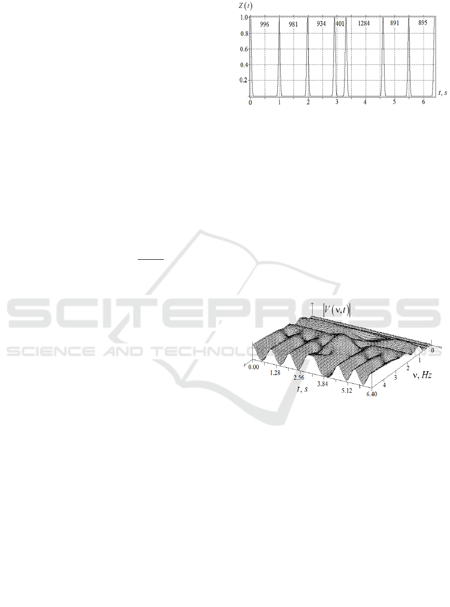
Let us consider a sequence of 𝑁=7 heartbeats,
which is a vector 𝑅𝑅

= {996, 981, 934, 401, 1284,
891, 895}, where all 𝑅𝑅

have millisecond dimension
(Fig.1).
Among 𝑅𝑅

values, 𝑛 = 0,1,2,…𝑁 − 1, 𝑡

=0,
there is a premature cardiac contraction, preceded by
the interval 𝑅

= 401 𝑚𝑠. Thus, we fix the only
extrasystole with the beat number 𝑛=
4 in the series. After a strong non-stationarity
𝑅

= 401 𝑚𝑠, a long compensatory pause
𝑅𝑅
(
0
)
= 1284 𝑚𝑠 occurs, and 𝑅𝑅
(
0
)
≫𝑅𝑅

.
Note that real cardiac contractions are located on an
uneven grid of discrete times 𝑡

(Bozhokin &
Suslova, 2014; Bozhokin et al., 2012, 2020, 2018).
Fig.1 shows frequency-modulated signal
𝑍
(
𝑡
)
(FMS) related to the tachogram with a single
extrasystole 𝑅

= 401 𝑚𝑠 and the time of
premature heartbeat 𝑡

=3.31 𝑠. In this signal, the
heart contractions occur at time moments 𝑡

=
𝑡

+𝑅𝑅

, where 𝑅𝑅

are determined by 𝑅𝑅

.
Fig.1 clearly indicates the difference between
frequency modulated signal (FMS) used in this article
and amplitude modulated signal (AMS) considered in
the Standards (Electrophysiology, 1996).
Figure 1: Continuous model of FMS for the tachogram with
a single extrasystole 𝑅

=401 ms.
The analytical expression
|
𝑉
(
𝜈,𝑡
)|
of the
continuous wavelet transform with the Morlet mother
wavelet function, where 𝜈 is the frequency, measured
in Hz, and 𝑡 is the time in s, was derived for the
irregular system of Gaussian peaks in (Bozhokin &
Suslova, 2014; Bozhokin et al., 2012, 2020, 2018).
Fig.2 shows the wavelet spectrum
|
𝑉
(
𝜈,𝑡
)|
for the
continuous signal 𝑍
(
𝑡
)
(Fig.1) in time-frequency
domain. We use the Morlet mother wavelet function
in the continuous wavelet transform (CWT) because
such a wavelet gives the correct positions of the
maxima in frequency and time for simplest non-
stationary signals.
Figure 2: CWT for the system of Gaussian peaks (Fig.1),
where 𝜈 is measured in Hz, and 𝑡 in s.
The frequency corresponding to the maximum
value of
|
𝑉
(
𝜈,𝑡
)|
is found. This so-called local
(instantaneous) frequency 𝐹

(
𝑡
)
depends on time.
Although the usual sinus rhythm contains both
spectral components of low-frequency VLF= (0.015;
0.04 Hz), mid-frequency LF= (0.04;0.15 Hz), and
high-frequency HF= (0.15; 0.4 Hz), the calculations
of 𝐹

(
𝑡
)
in this case do not lead to great
difficulties (Bozhokin & Suslova, 2014; Bozhokin et
al., 2012, 2020, 2018). However, in the case of
extrasystole (Fig.1), the behavior of
|
𝑉
(
𝜈,𝑡
)|
(Fig.2)
near the extraordinary time moment 𝑡

=3.31 𝑠 has
more complex nature. This entails difficulties in
calculating the local frequency 𝜈=𝐹

(
𝑡
)
near the
critical time moment 𝑡

= 3.31 𝑠. To calculate
𝐹

(
𝑡
)
for a signal with an ectopic Gaussian peak,
BIOSIGNALS 2025 - 18th International Conference on Bio-inspired Systems and Signal Processing
1040

we should formulate criteria that will determine upper
𝐹

(
𝑡
)
and lower 𝐹

(
𝑡
)
limits for local frequency
𝐹

(
𝑡
)
:
𝐹

(
𝑡
)
≤𝐹

(
𝑡
)
≤𝐹

(
𝑡
)
. The difficulties
in determining the boundaries 𝐹

(
𝑡
)
and 𝐹

(
𝑡
)
are
due to the fact that in the model of the signal 𝑍
(
𝑡
)
as
a set of Gaussians (Fig.1), along with the first
frequency harmonic, which gives the maximum
|
𝑉
(
𝜈,𝑡
)|
, there appear senior harmonics, which also
give maxima to
|
𝑉
(
𝜈,𝑡
)|
. In addition, we have the
tachogram with extrasystoles (Fig.1), where time
intervals 𝑅𝑅

between the peaks change significantly
in time. This leads to a complex system of
|
𝑉
(
𝜈,𝑡
)|
maximal values. We are interested in the position of
the first harmonic, which determines the basic
frequency of the heart rate. Let us formulate an
algorithm for finding 𝐹

(
𝑡
)
for a signal with
ectopic heartbeats. We will consider as ectopic the
interval 𝑅𝑅

preceding the moment 𝑡

of the
heartbeat if the duration between the peaks of
neighboring Gaussians satisfies the condition
𝑅𝑅

<0.65 𝑠 (Shubik & Tikhonenko, 2019)
(Shubik & Tikhonenko, 2019). First, using the known
values of 𝑅𝑅

, we calculate the corresponding local
frequencies 𝑓

=



, where the values of 𝑓

have the
dimension Hz, and the values of 𝑅𝑅

are measured in
seconds. Our first assumption is that in the time
interval close to the ectopic Gaussian peak, the value
𝐹

(
𝑡
)
should be approximately equal to 𝑓

. This
physical principle can be formulated in a simple way.
If there is a short time interval 𝑅𝑅

between
Gaussian peaks, then the first harmonic of such a
signal (the sum of identical Gaussian peaks) cannot
be greater than
1
𝑅𝑅


.
However, if we have a case of several successive
ectopic peaks (near the ectopic peak 𝑅𝑅

=𝑅𝑅

there are other ectopic peaks with small 𝑅𝑅

values),
then the behavior of local frequency 𝐹

(
𝑡
)
will also
depend on the subsequent compensatory pause and
neighboring ectopic intervals. Therefore, the
algorithm to determine 𝐹

(
𝑡
)
at 𝑡≈𝑡

must
depend on the neighboring cardiac intervals, that is,
on 𝑅𝑅

,𝑅𝑅

and 𝑅𝑅

,𝑅𝑅

, and,
consequently, on the adjacent moments of time 𝑡

,
𝑡

and 𝑡

,𝑡

. It becomes especially important
when a long compensatory pause followers a short
ectopic interval of extrasystole. The proposed
algorithm to calculate the local frequency 𝐹

(
𝑡
)
should work both for a normal sine rhythm without
ectopic intervals, and for a sequence of Gaussian
peaks with several ectopic intervals 𝑅𝑅

.
Let us consider the limits 𝑓


and 𝑓


for
finding discrete local frequencies on 𝑛 - time interval.
In this case, the upper 𝑓


and lower 𝑓


boundaries of the discrete local frequencies 𝑓

=



can be determined from the relations
𝑓


=

1+𝐵
(
𝑅𝑅

)

𝑓

, (3)
𝑓


=
(
1−𝐴
)
𝑓

. (4)
Note that the upper limit of the frequency search
corridor 𝑓


depends on 𝑅𝑅

measured in seconds.
The formula for 𝐵
(
𝑅𝑅

)
, which is the relative excess
of 𝑓


over the value of 𝑓

, was derived while
analyzing the ectopic intervals given in (Shubik &
Tikhonenko, 2019). The lower limit 𝐴 of the search
for 𝐹

(
𝑡
)
, which characterizes the difference
between 𝑓


and 𝑓

in (4), is a constant value 𝐴=
0.25.
𝐵
(
𝑅𝑅

)
=𝐵

+














, (5)
where 𝑅𝑅

is measured in s, 𝐵

=0.001; 𝐵
ах
=0.21;
𝑅𝑅

=0.840 s, 𝜏

=0.12 s.
The given numerical data were obtained from the
analysis of approximately 70 tachogram records with
various cardiac dysfunctions (Shubik & Tikhonenko,
2019).
For short (extrasystolic) time intervals 𝑅𝑅

≈
0.4 𝑠, the excess 𝐵
(
𝑅𝑅

)
of the discrete 𝑓


over
𝑓

has a small value 𝐵
(
𝑅𝑅

)
<<1. For long time
intervals 𝑅𝑅

≫1.4 𝑠, the value of 𝐵
(
𝑅𝑅

)
reaches
its asymptotic value 𝐵
ах
=0.21. Thus, at 𝑅𝑅

≤
𝑅𝑅

, the upper search limit 𝑓


for the continuous
function 𝑓

(
𝑡
)
slightly exceeds the discrete
frequency 𝑓

=



. For such intervals 𝑓


=
1.001𝑓

. For intervals with 𝑅𝑅

>1.4 𝑠, the
discrete upper search boundary tends to 𝑓


=
1.21𝑓

. Note that after the ectopic interval 𝑅𝑅

=
𝑅𝑅

= 0.401 𝑠 with number 𝑛, we observe long
compensatory pause 𝑅𝑅

= 1.284 𝑠 with number
𝑛+1. As a result, the ratio of adjacent local
frequencies will also be large




=




≈3.2.
Consequently, the constant A, which determines the
lower search limit for the local frequency, should be
increased to the value 𝐴=0.7.
Heart Rate Turbulence: Wavelet Analysis of Frequency Modulated Signals
1041

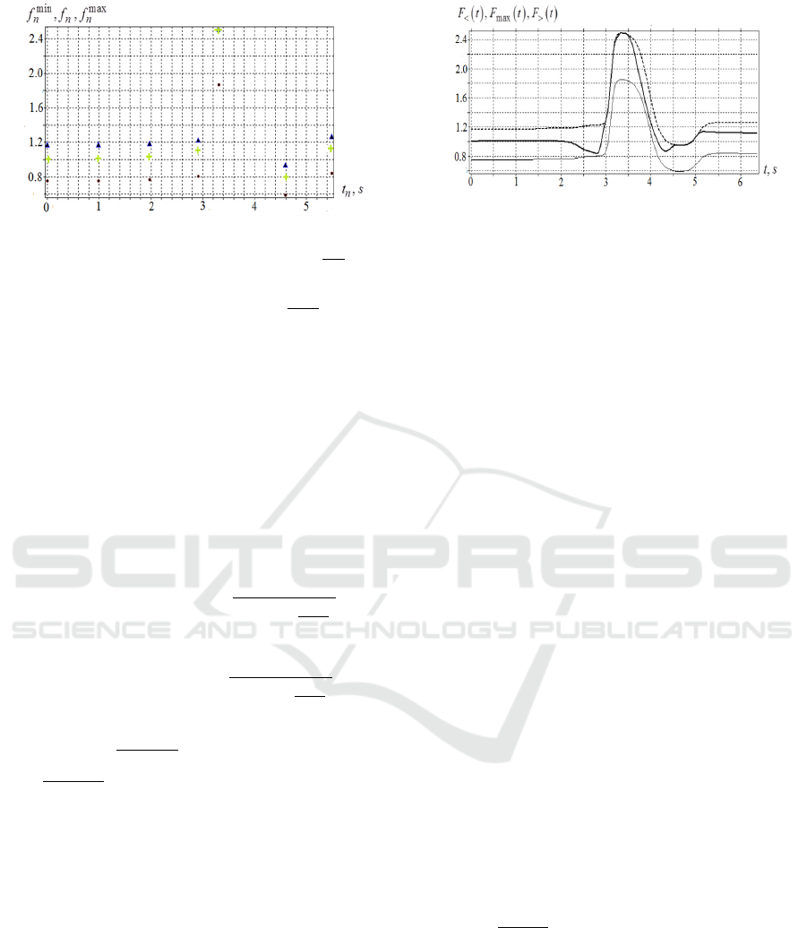
Figure 3: Time dependence of discrete local frequencies for
𝑅𝑅

tachogram: 𝑓


are indicated by dots, 𝑓

=



− by
crosses, 𝑓


− by triangles. For 𝑡=𝑡

= 3.31 𝑠 (the
moment of ectopic heartbeat) 𝑓


=𝑓

=



.
Fig.3 shows the discrete local frequencies for the
sequence of cardio intervals in the 𝑅𝑅

record.
The next task is to find new smooth boundaries
𝐹

(
𝑡
)
and 𝐹

(
𝑡
)
depending on time continuously in
the interval 0 ≤ 𝑡 ≤ 𝑇 (𝑇 is the observation period
for the signal), based on 𝑓


and 𝑓


frequencies
specified for discrete 𝑛. The required formulas for
upper 𝐹

(
𝑡
)
and lower 𝐹

(
𝑡
)
continuous boundaries
of the local frequency have the form of sigmoid
functions
𝐹

(
𝑡
)
=𝑓


+
∑















, (6)
𝐹

(
𝑡
)
=𝑓


+
∑















, (7)
where 𝑡


=
(




)

is the center of the interval;
𝜏

=
(




)

=𝑅𝑅

/10 is the characteristic time
depending on the duration of the interval between
heartbeats. If the time interval ends with extrasystole
𝑅𝑅

= 0.401 𝑠, then the characteristic time 𝜏

will
be small 𝜏

≈ 0.04 𝑠. If the time interval ends with
compensatory pause 𝑅𝑅

= 1.284 𝑠, then the
transition region will be large 𝜏

≈0.13 𝑠.
Approximation by smooth sigmoid functions has
an advantage over approximations using splines. In
the case of strong heterogeneity in the position of
discrete points, spline approximation leads to strong
oscillation of a smooth curve for intermediate values
of the argument.
Figure 4: Dependence on time of the lower limit of
frequency search 𝐹

(
𝑡
)
(thin line), the sought local
frequency 𝐹

(
𝑡
)
(thick line), and the upper limit of
frequency search 𝐹

(
𝑡
)
(dashed line) for tachogram 𝑅𝑅

The final step is to determine 𝐹

(
𝑡
)
by finding
the maximum of
|
𝑉
(
𝜈,𝑡
)|
(CWT of frequency
modulated signal 𝑍(𝑡)). Fig.4 shows the frequency
corridor 𝐹

(
𝑡
)
≤𝐹

(
𝑡
)
≤𝐹

(
𝑡
)
for local
(instantaneous) frequency 𝐹

(
𝑡
)
in the case of a
single extrasystole 𝑅𝑅

= 0.401 𝑠 with
compensatory pause 𝑅𝑅
(
0
)
= 1284 𝑚𝑠.
2.3 Algorithm for Calculating Local
Frequency in the Case of a
Tachogram with Three
Extrasystoles
Let us apply the algorithm to determine 𝐹

(
𝑡
)
in
the case of tachograms with multiple ectopic
intervals. As an example, we consider the tachogram
record 𝑅𝑅

= {1072, 544, 1056, 552, 1124, 548,
1129} with three extrasystoles:
𝑅𝑅

(
1
)
=
544 𝑚𝑠
, 𝑅𝑅

(
2
)
= 552 𝑚𝑠,
𝑅𝑅

(
3
)
= 548 𝑚𝑠
given in (Shubik & Tikhonenko, 2019). Each of the
extrasystoles is followed by the compensatory pause.
The processing sequence of such a tachogram
𝑅𝑅

is similar to the example of the tachogram
𝑅𝑅

discussed above. The analysis of |𝑉
(
𝜈,𝑡
)
| (CWT
for the tachogram 𝑅𝑅

) shows the existence of three
vertices 𝑖=3 located at points with specific fixed
frequencies and times

𝜈

(
𝑖
)
,𝑡

(
𝑖
)

, measured in
Hz and s, respectively. These vertices relate to the
extrasystoles with the characteristic frequency
𝜈

(
𝑖
)
=



(

)
.
Here we have {𝜈

(
1
)
= 1.838 𝐻𝑧, 𝑡

(
1
)
=
1.616 𝑠}; {𝜈

(
2
)
= 1.811 𝐻𝑧, 𝑡

(
2
)
=
3.224 𝑠}; {𝜈

(
3
)
= 1.825 𝐻𝑧, 𝑡

(
3
)
=
4.896 𝑠}.
BIOSIGNALS 2025 - 18th International Conference on Bio-inspired Systems and Signal Processing
1042

Figure 5: Dependence on time of the lower limit of
frequency search 𝐹

(
𝑡
)
(thin line), the sought local
frequency 𝐹

(
𝑡
)
(thick line), and the upper limit of
frequency search 𝐹

(
𝑡
)
(dashed line) for tachogram 𝑅𝑅

.
The a
nalysis of Fig.5 reveals a sharp increase in
the sought local frequency 𝐹

(
𝑡
)
at the moments of
extrasystoles for the 𝑅𝑅

tachogram with three
extrasystoles, and then a decrease during the
subsequent compensatory pauses. Three maxima of
the continuous function 𝐹

(
𝑡
)
exactly correspond
to the discrete values

𝜈

(
𝑖
)
,𝑡

(
𝑖
)

. Based on the
processing of the data taken from (Shubik &
Tikhonenko, 2019), we can conclude that each
individual extrasystole, characterized by its own
interval and compensatory pause, differs from
another extrasystole in the duration and the range of
oscillations of the corresponding local frequency
function. Thus, the time behavior of local frequency
near extrasystoles is closely related to the properties
of extrasystoles. This fact can serve as a basis for
classifying ectopic beats.
3 DISCUSSION
For many functional tests (bicycle ergometry,
treadmill, orthostatic, respiratory, glucose-tolerant,
pharmacological, and psychoemotional tests) the
quantitative description of non-stationary heart rate
variability (HRV) is of great importance. The non-
stationary nature of HRV is reflected in the
significant dependence of spectral and statistical
properties of the processed signals on time. It is
especially difficult to process HRV signals with
extrasystoles - premature contractions of the heart, in
which the local (instantaneous) frequency of the
signal changes by 3-4 times over a time interval of
𝑅𝑅

≈0.5 𝑠. As a basis for the analysis of HRV
with extrasystoles, this paper uses frequency-
modulated signal model (FMS) instead of the
traditional amplitude-modulated signal model
(AMS). AMS tachogram model (Electrophysiology,
1996) assumes that peaks of different heights 𝑅𝑅

are
uniformly located at a time grid, and separated by
equal time intervals ∆𝑡 = 𝑅𝑅𝑁𝑁, where the
𝑅𝑅𝑁𝑁 value is the average duration of 𝑅𝑅

intervals
over the entire observation period. Frequency
modulated signal (FMS) is a set of identical Gaussian
peaks whose centers are located on an uneven time
grid and coincide in time with the true moments of
heartbeats 𝑡

=𝑡

+𝑅𝑅

,𝑛=0,1,2,…𝑁−1,
𝑁 is the number of heartbeats. In contrast to AMS
model, FMS model used in the article makes it
possible to find the true frequencies of heart rate
oscillations. The differences between traditional
AMS model and FMS model are especially noticeable
when analyzing functional tests, in which the
tachogram trend is clearly visible over the entire
testing period
In this paper, we propose to analyze the time
behavior of local (instantaneous) frequency 𝐹

(
𝑡
)
as a new characteristic of the heart rhythm with strong
non-stationarity (arrhythmia, extrasystole). The
behavior in time of the continuous signal 𝐹

(
𝑡
)
shows both the presence of extrasystoles and their
difference from each other.
An essential advantage of this approach is in the
fact that FMS model allows us to obtain an analytical
expression for the continuous wavelet transform
(CWT) with the Morlet mother wavelet function. The
analytical expression for the wavelet spectrum allows
for the efficient calculation and analysis of the local
frequency function.
The advantage of considering local frequency as a
new characteristic of the tachogram becomes relevant
when studying various cardiac arrhythmias. In this
case the normal sinus rhythm is disrupted and the true
moments of cardiac contractions become important.
An important application of the method proposed in
this article is the study of single and repeated
extrasystoles associated with the appearance of an
ectopic focus of trigger activity, as well as with the
existence of a repeated reverse excitation entry (re-
entry mechanism). The behavior of local frequency
function over time is different for different types of
ectopic beats. Therefore, this characteristic can serve
as a basis for classifying arrhythmias.
The main
prognostic parameters for HRT are: TO - the onset of
extrasystole and TS - the extrasystole slope, which do
not take into account the extrasystoles themselves and
subsequent compensatory pauses, namely 𝑅𝑅

and
𝑅𝑅
(
0
)
intervals. We believe that the study of HRT
should include the intervals of the extrasystole and
the compensatory intervals, as they contain important
information about the characteristic features of the
rhythm disturbance.
Heart Rate Turbulence: Wavelet Analysis of Frequency Modulated Signals
1043

4 CONCLUSIONS
The article proposes a mathematical model in which
the tachogram signal is considered as FMS
(frequency-modulated signal), which is a
superposition of identical Gaussian peaks. The
maxima of the Gaussian peaks are located at the
moments of real heart contractions. To study HRT
(heart rate turbulence), both the durations of the
ectopic intervals between the peaks 𝑅𝑅

and the
duration of the subsequent compensatory pauses
𝑅𝑅
(
0
)
are taken into account.
For quantitative analysis of HRT, we propose to
calculate the time behavior of local frequency
𝐹

(𝑡) at any time both before and after ectopic
beats. This allows us to classify the ectopic intervals
and subsequent compensatory pauses. In the change
of 𝐹

(𝑡), one can identify a trend, as well as
fluctuations relative to this trend.
The proposed method based on the analysis of
local heart rate can be applied to study non-stationary
cardiac tachograms of various patients with normal
sinus rhythm both at rest and during functional tests.
We can also propose to use the developed method for
classification of cardiac rhythm with ectopic intervals
for patients suffering from congestive heart failure
(CHF), atrial fibrillation (AF), atrial premature
contraction (APC), ventricular premature contraction
(VPC), left bundle branch block (LBBB),
ischemic/dilated cardiomyopathy (ISCH) and sick
sinus syndrome (SSS).
ACKNOWLEDGEMENTS
The research is funded by the Ministry of Science and
Higher Education of the Russian Federation as part of
the World-class Research Center program: Advanced
Digital Technologies (contract No. 075-15-2022-311
dated 20.04.2022)
REFERENCES
Schmidt, G., Malik, M., Barthel, P., Schneider, R., Ulm, K.,
Rolnitzky, L., ... & Schömig, A. (1999). Heart-rate
turbulence after ventricular premature beats as a
predictor of mortality after acute myocardial infarction.
The Lancet, 353(9162), 1390-1396.
Bauer, A., Malik, M., Schmidt, G., Barthel, P., Bonnemeier,
H., Cygankiewicz, I., ... & Zareba, W. (2008). Heart
rate turbulence: standards of measurement,
physiological interpretation, and clinical use:
International Society for Holter and Noninvasive
Electrophysiology Consensus. Journal of the American
College of Cardiology, 52(17), 1353-1365.
Disertori, M., Masè, M., Rigoni, M., Nollo, G., & Ravelli,
F. (2016). Heart rate turbulence is a powerful predictor
of cardiac death and ventricular arrhythmias in
postmyocardial infarction and heart failure patients: a
systematic review and meta-analysis. Circulation:
Arrhythmia and Electrophysiology, 9(12), e004610.
MA, W. (2004). Heart rate turbulence: a 5-year review.
Heart Rhythm, 1, 732-738.
Cygankiewicz, I., & Zaręba, W. (2006). Heart rate
turbulence-an overview of methods and applications.
Cardiology Journal, 13(5), 359-368.
Cygankiewicz, I. (2013). Heart rate turbulence. Progress in
cardiovascular diseases, 56(2), 160-171.
Germanova, O., Shchukin, Y., Germanov, V., Galati, G., &
Germanov, A. (2021). Extrasystolic arrhythmia: is it an
additional risk factor of atherosclerosis? Minerva
Cardiology and Angiology, 70(1), 32-39.
Huikuri, H. V., Castellanos, A., & Myerburg, R. J. (2001).
Sudden death due to cardiac arrhythmias. New England
Journal of Medicine, 345(20), 1473-1482.
Zeid, S., Buch, G., Velmeden, D., Söhne, J., Schulz, A.,
Schuch, A., ... & Wild, P. S. (2024). Heart rate
variability: Reference values and role for clinical
profile and mortality in individuals with heart failure.
Clinical Research in Cardiology, 113(9), 1317-1330.
Thayer, J. F., Yamamoto, S. S., & Brosschot, J. F. (2010).
The relationship of autonomic imbalance, heart rate
variability and cardiovascular disease risk factors.
International journal of cardiology, 141(2), 122-131.
Kubota, Y., Chen, L. Y., Whitsel, E. A., & Folsom, A. R.
(2017). Heart rate variability and lifetime risk of
cardiovascular disease: the Atherosclerosis Risk in
Communities Study. Annals of epidemiology, 27(10),
619-625.
Huikuri, H. V., & Stein, P. K. (2013). Heart rate variability
in risk stratification of cardiac patients. Progress in
cardiovascular diseases, 56(2), 153-159.
Turcu, A. M., Ilie, A. C., Ștefăniu, R., Țăranu, S. M., Sandu,
I. A., Alexa-Stratulat, T., ... & Alexa, I. D. (2023). The
impact of heart rate variability monitoring on
preventing severe cardiovascular events. Diagnostics,
13(14), 2382.
Yan, S. P., Song, X., Wei, L., Gong, Y. S., Hu, H. Y., & Li,
Y. Q. (2023). Performance of heart rate adjusted heart
rate variability for risk stratification of sudden cardiac
death. BMC Cardiovascular Disorders, 23(1), 144.
Lombardi, F., & Stein, P. K. (2011). Origin of heart rate
variability and turbulence: an appraisal of autonomic
modulation of cardiovascular function. Frontiers in
Physiology, 2, 95.
Blesius, V., Schölzel, C., Ernst, G., & Dominik, A. (2020).
HRT assessment reviewed: a systematic review of heart
rate turbulence methodology. Physiological
Measurement, 41(8), 08TR01.
Rajendra Acharya, U., Paul Joseph, K., Kannathal, N., Lim,
C. M., & Suri, J. S. (2006). Heart rate variability: a
review. Medical and biological engineering and
computing, 44, 1031-1051.
BIOSIGNALS 2025 - 18th International Conference on Bio-inspired Systems and Signal Processing
1044

Sauerbier, F., Haerting, J., Sedding, D., Mikolajczyk, R.,
Werdan, K., Nuding, S., ... & Kluttig, A. (2024). Impact
of QRS misclassifications on heart-rate-variability
parameters (results from the CARLA cohort study).
PloS one, 19(6), e0304893.
Yin, D. C., Wang, Z. J., Guo, S., Xie, H. Y., Sun, L., Feng,
W., ... & Qu, X. F. (2014). Prognostic significance of
heart rate turbulence parameters in patients with chronic
heart failure. BMC cardiovascular disorders, 14, 1-8.
Koyama, J., Watanabe, J., Yamada, A., Koseki, Y., Konno,
Y., Toda, S., ... & Shirato, K. (2002). Evaluation of
heart-rate turbulence as a new prognostic marker in
patients with chronic heart failure. Circulation journal,
66(10), 902-907.
Tsvetnikova, A.A., Bernhard,t E.R., Parmon, E.V., Aseev,
A.V., Treshkur, T.V.. (2008). Turbulentnost’
serdechnogo ritma: metodicheskie aspekty (Inkart,
SPb.) (in Russian).
Electrophysiology, T. F. O. T. E. S. O. C. T. N. A. S. O. P.
(1996). Heart rate variability: standards of
measurement, physiological interpretation, and clinical
use. Circulation, 93(5), 1043-1065.
Milaras, N., Dourvas, P., Doundoulakis, I., Sotiriou, Z.,
Nevras, V., Xintarakou, A., ... & Gatzoulis, K. (2023).
Noninvasive electrocardiographic risk factors for
sudden cardiac death in dilated cardiomyopathy: is
ambulatory electrocardiography still relevant? Heart
Failure Reviews, 28(4), 865-878.
Bozhokin, S. V., Suslova, I. B. (2014). Analysis of non-
stationary HRV as a frequency modulated signal by
double continuous wavelet transformation method.
Biomedical Signal Processing and Control, 10, 34-40.
Bozhokin, S. V., Lesova, E. M., Samoilov, V. O.,
Tolkachev, P. I., (2012) Wavelet Analysis of
Nonstationary Heart Rate Variability in a Head-Up Tilt-
Table Test, Biophysics, 57(4), 530-543.
Bozhokin, S. V., Lesova, E. M., Samoilov, V. O., &
Barantsev, K. A. (2020). Nonstationary heart rate
variability during the head-down tilt test. Biophysics,
65, 151-158.
Bozhokin S. V., Lesova E. M., Samoilov V. O., Tarakanov
D. E. (2018) Nonstationary heart rate variability in
respiratory tests, Human Physiology, 44(1), 32-40.
Addison, P. S. (2005). Wavelet transforms and the ECG: a
review. Physiological measurement, 26(5), R155.
Cartas-Rosado, R., Becerra-Luna, B., Martínez-Memije,
R., Infante-Vazquez, O., Lerma, C., Perez-Grovas, H.,
& Rodríguez-Chagolla, J. M. (2020). Continuous
wavelet transform based processing for estimating the
power spectrum content of heart rate variability during
hemodiafiltration. Biomedical Signal Processing and
Control, 62, 102031.
Wang, T., Lu, C., Sun, Y., Yang, M., Liu, C., & Ou, C.
(2021). Automatic ECG classification using continuous
wavelet transform and convolutional neural network.
Entropy, 23(1), 119.
Shubik, Yu.V., Tikhonenko, V.M. (2019). Holter
monitoring for arrhythmia. Kholterovskoe
monitorirovanie pri aritmiyakh. OOO”Nevskij rakurs“,
Saint-Petersburg,(in Russian).
Heart Rate Turbulence: Wavelet Analysis of Frequency Modulated Signals
1045