Deep Neural Network Architectures for Advanced Hiking Map

Generation

Olivier Schirm

, Maxime Devanne

, Jonathan Weber

, Arnaud Lecus

Germain Forestier

and C

edric Wemmert

ICube, University of Strasbourg, Strasbourg, France

IRIMAS, University of Haute Alsace, Mulhouse, France

Visorando, Soultz-Haut-Rhin, France

Keywords:

Hiking Maps Generation, GPS Trajectories, Convolutional Neural Network, Map Inference.

Abstract:

The automation of hiking map generation using deep learning represents a pivotal advancement in geospa-

tial analysis. This study investigates the application of neural network architectures to derive accurate hiking

maps from GPS trajectory data, exclusively collected via the Visorando mobile application. By exploring the

utility of 17 distinct raster features derived from geospatial data, we identify the heatmap as the most effective

input for mapping intricate trail networks, achieving superior performance across accuracy, segmentation, and

connectivity metrics. Among various architectures evaluated, HRNet emerged as the most efﬁcient model,

demonstrating exceptional results when combined with optimal input features, signiﬁcantly outperforming

state-of-the-art approaches in intersection detection and trail segmentation. This research introduces a novel

framework for converting vector-based GPS traces into rasterized data suitable for convolutional neural net-

works, overcoming challenges like noisy inputs and terrain variability. The ﬁndings establish a new benchmark

for efﬁciency and accuracy in hiking map generation, offering valuable insights for the broader ﬁeld of au-

tomated map inference reliant on GPS data. Future work will explore direct spatio-temporal processing of

vector data, eliminating raster conversion for enhanced scalability and precision.

1 INTRODUCTION

In recent years, GPS trajectory data has been widely

used in various ﬁelds, such as analyzing travel pat-

terns (He et al., 2020; Li et al., 2021), transportation

ﬂow analysis (Ruan et al., 2020a), predicting travel

times (Chen et al., 2022) or tracking animal move-

ments (Roy et al., 2022). This study focuses on us-

ing crowdsourced GPS trajectories to create hiking

maps. According to a comprehensive review on map

inference from GPS trajectories (Chao et al., 2020),

there are three main techniques: road abstraction,

incremental branching, and intersection connection.

However, with recent advances in map inference, it is

worth considering deep learning as a fourth category.

Additionally, some methods, like elongated ribbon

generation, centerline extraction, and skeletonization

proposed in (Dal Poz et al., 2022), do not ﬁt neatly

into these four categories.

Road abstraction focuses on identifying dense

areas of GPS data to extract road networks using clus-

tering algorithms. This method usually involves three

main steps: preparing the data, applying clustering,

and generating the road map. Various clustering tech-

niques, like k-means and KDE-based clustering, have

been used to create these maps. The survey highlights

three key methods: RA-K-MEANS (Stanojevic et al.,

2018), RA-TOPIC (Zheng et al., 2017), and RA-KDE

(Biagioni and Eriksson, 2012b), which is seen as pio-

neering work in the ﬁeld. Each of these methods uses

different strategies and optimizations for map genera-

tion. A more recent approach proposed in (Guo et al.,

2021) builds a road network through four steps: cre-

ating a density surface, compressing it, constructing

an initial road network, and reﬁning it using edge

weights. After the survey, another method (Yang

et al., 2020) added valuable insights by focusing on

pedestrian data. Additionally, (Prabowo et al., 2019)

proposed an Iterated Trajectory Mean Shift Sampling

method.

Incremental branching builds a map by grad-

ually adding new roads to an initially empty map

until all GPS trajectories are processed. There are

two main approaches: Trace Merging and Map Ex-

Schirm, O., Devanne, M., Weber, J., Lecus, A., Forestier, G. and Wemmert, C.

Deep Neural Network Architectures for Advanced Hiking Map Generation.

DOI: 10.5220/0013351700003905

Paper published under CC license (CC BY-NC-ND 4.0)

In Proceedings of the 14th International Conference on Pattern Recognition Applications and Methods (ICPRAM 2025), pages 531-541

ISBN: 978-989-758-730-6; ISSN: 2184-4313

531

panding. Trace Merging adds new trajectories to

the map by merging them with existing roads based

on distance measures. In contrast, Map Expanding

starts from a known map point and extends the map

by inferring new roads from the trajectories passing

through that point. The survey highlights two key

studies: IB-TM (Ahmed and Wenk, 2012), which

follows the trace merging approach, and IB-ME (He

et al., 2018), which focuses on map expanding. A

more recent method introduced in (Fu et al., 2020)

estimates road centerlines based on GPS trajectory

density, merging them incrementally to form a road

network. This method uses kernel density analysis

and Gaussian distribution ﬁtting to extract centerlines,

which are then merged and reﬁned. One of the ear-

liest efforts using incremental branching techniques

was presented in (Cao and Krumm, 2009).

Intersection connection methods focus on accu-

rately detecting intersections and linking them using

GPS trajectory data. These approaches identify in-

tersections by analyzing movement patterns or point

density. The typical steps include: 1) scanning trajec-

tory points and identifying sequences near intersec-

tions based on heading and speed; 2) clustering in-

tersection points based on proximity or turn patterns

to deﬁne intersection areas; and 3) connecting inter-

sections using trajectories, while considering the type

of intersection for establishing the links. IL-TURN

(Karagiorgou and Pfoser, 2012) is a key example of

this approach. Recent studies, such as (Alsahﬁ et al.,

2020), use the Douglas-Peucker algorithm to identify

intersections, while (Guo et al., 2022) applies Otsu-

based detection and trajectory clustering based on dis-

tance and direction. Additionally, (Zhou et al., 2022)

use different ﬁtting methods to handle sparse or un-

even GPS data, and (Zhang et al., 2021) employ the

CFDP algorithm for precise intersection detection.

CNN centerline segmentation represents the lat-

est and most advanced method for map inference

using GPS trajectories. This approach has gained

prominence with the rise of deep learning tech-

niques, which became more common after the orig-

inal survey. Initially, deep learning was applied to

edge pruning in map inference algorithms, as shown

in (Prabowo et al., 2019). Later, deep learning mod-

els were combined with both aerial images and GPS

trajectories to improve map segmentation, as demon-

strated in (Sun et al., 2019), where crowd-sourced

GPS data alongside traditional aerial imagery were

used. Other studies, such as (Wu et al., 2020; Liu

et al., 2022), also explore this combination. An alter-

native approach in (Zhang et al., 2020) used Convolu-

tional Neural Networks (CNNs) to generate training

data from GPS trajectories with aerial images as sup-

plementary information. Some studies focus purely

on using deep learning with aerial images for map in-

ference, without GPS data, as in (Zhu et al., 2021;

Abdollahi et al., 2020). In contrast, this paper cen-

ters exclusively on inferring road maps from GPS tra-

jectories, without relying on additional features like

aerial imagery. Key studies in this area include (Ruan

et al., 2020b), (Feng et al., 2020), and (Eftelioglu

et al., 2022), which present signiﬁcant advancements

in generating road maps purely from GPS data.

In this work, we aim to advance the state of auto-

mated map generation by addressing these challenges

through a deep learning approach tailored to GPS

data. Our primary objective is to explore the efﬁcacy

of various CNN architectures and input features for

generating detailed hiking maps, without relying on

supplementary data such as aerial imagery. By focus-

ing on GPS trajectories recorded via the Visorando

application, we seek to establish a robust framework

for accurate and efﬁcient map inference in diverse ter-

rains, including dense forests or mountains. The main

contributions of this paper are outlined below:

• Conducting a comprehensive review of the latest

techniques in utilizing CNNs for image data, with

a particular focus on the innovative integration of

GPS trace data as a novel source of multiple types

of information, enriching current methodologies

in the ﬁeld.

• Designing a structured series of experiments to

rigorously evaluate the most effective combina-

tions of diverse information sets as inputs for

CNNs. This approach enables a more precise

method for leveraging various data sources in the

merging of GPS traces through CNN applications.

• Identifying, through empirical studies, the opti-

mal input composition for the model, setting a

new performance benchmark on our dataset and

advancing the state of the art in automated hiking

map generation.

• Evaluating the best architecture on a real dataset

consisting of traces collected by hikers using the

Visorando mobile application

2 MATERIALS AND METHODS

2.1 Data

In this work, we address the challenge of generating

hiking maps from GPS trajectories using deep learn-

ing. Our model is trained on a dataset provided by

https://www.visorando.com/

ICPRAM 2025 - 14th International Conference on Pattern Recognition Applications and Methods

532

Visorando, comprising thousands of GPS tracks col-

lected by users during outdoor activities across di-

verse geographical areas (see Table 1). These user-

generated GPS traces, recorded with personal de-

vices, contain varying levels of noise due to uncon-

trolled conditions, including the possibility of tracks

captured while driving. For example, the Blaesheim

dataset, close to a highway, exhibits higher average

speeds, which our method accounts for by adapting

to different user behaviors and trace qualities. We

release the dataset used in this study

to ensure the

reproducibility of our work and offer practitioners a

valuable, rare resource of real-world hiking GPS data

for future developments.

The following sections describe our data prepro-

cessing pipeline, including augmentation and conver-

sion to raster format, and the use of convolutional

neural networks (CNNs) to infer road networks from

GPS data. We also present our evaluation framework

and performance metrics.

2.2 Data Preparation

2.2.1 Traces and Characteristics

We ﬁrst introduce the data preparation in order to

deﬁne what are traces and how can we feed them

to contain more information that will be useful in

the rest of the method. Let T = t

, . . . ,t

a collection of GPS traces, where each trace t

is a sequence of GPS points (lat, lon) like t

(lat

i,1

, lon

i,1

), (lat

i,2

, lon

i,2

), . . . , (lat

i,n

, lon

i,n

). Most

of the time, traces have a third characteristic referred

to as time

i, j

, which is the precise timestamp when the

point has been recorded. If time is speciﬁed in the

input, it is possible to compute the speed and the ac-

celeration in a trace.

When comparing two consecutive points

i, j−1

= (lat

i, j−1

, lon

i, j−1

, time

i, j−1

) and

i, j

= (lat

i, j

, lon

i, j

, time

i, j

), speed is the dif-

ference between point positions and times:

speedi, j =

distance(p

i, j−1

i, j

)

∆time(p

i, j−1

i, j

)

. When comparing these

two points with a third one, it is possible to compute

the acceleration: acceleration

i, j

∆speed(pi, j−1, p

i, j

)

∆time(p

i, j−1

i, j

)

Leaving the time attribute, it is possible to compare

two points to know the heading of a point ∠ p

i, j

i, j+1

The resulting values will be in a [−180;180] range.

Lastly, a bearing difference between points can be

deduced from this previous computation with the

https://ﬁgshare.com/articles/dataset/Deep Neural

Network Architectures for Advanced Hiking Map

Generation/25152698

following equations:

∠p

i, j

i, j+1

(

∠p

i, j

i, j+1

+ 360, if ∠p

i, j

i, j+1

< 0

∠p

i, j

i, j+1

, otherwise

(1)

∆∠p

i, j

= min





∠p

i, j

i, j+1

− ∠ p

i, j−1

i, j



360 −



∠p

i, j

i, j+1

− ∠ p

i, j−1

i, j





(2)

2.2.2 Preprocessing

In addition to computing spatial and kinematic vari-

ables, it is essential to mitigate initial noise present in

T to enhance the quality and reliability of the analy-

sis. Firstly, we eliminate consecutive duplicate points

based on latitude and longitude, thereby reducing re-

dundancy that could signiﬁcantly affect subsequent

image generation. Secondly, we clean the traces by

identifying and removing each point whose the dis-

tance with its consecutive point exceeds 100 meters.

Such substantial jumps in distance are likely at-

tributable to GPS errors or signal loss, rather than

genuine movements. Lastly, we apply a stringent ﬁl-

ter to exclude points with speed values exceeding 10

km/h, preventing sudden GPS jumps within a 100-

meter range from affecting the analysis.

2.2.3 Raster Features

We chose to transform the geospatial time series into

raster data as our input format for two main reasons:

it is an image-like format that suits perfectly the input

requirements of a deep neuronal network, and it con-

tains geographical positioning information. Since our

data sources are initially provided in a vectorial GPX

format, we have to convert them to a raster. We aim

to construct a raster R of W × H × C size, where W

and H are the image dimensions, and C is the number

of features. Equation 3 shows how to compute W and

H from T , with r representing the chosen resolution.

Equation 4 shows how to ﬁnd the right position (x, y)

in R for a given latitude and longitude (lat

i, j

, lon

i, j

lon

max

= max

∈T



max

(lat,lon)∈t

(lon)



lon

min

= min

∈T



min

(lat,lon)∈t

(lon)



W =



lon

max

− lon

min



(3)

lat

max

= max

∈T



max

(lat,lon)∈t

(lat)



Deep Neural Network Architectures for Advanced Hiking Map Generation

533

Table 1: Comprehensive overview of the datasets used in experimental analysis.

Dataset Number of Mean distance Mean speed Bounding box Terrain

traces (km) (m/s) (lat/lon)

Labaroche 292 33.530 1.512 48.084–48.118, 7.183–7.245 mountain

Hunawihr 183 32.022 1.547 48.158–48.188, 7.282–7.326 vineyard

Ribeauville 2519 36.929 1.764 48.180–48.219, 7.250–7.319 vineyard

Linthal 3509 45.217 2.184 47.939–48.014, 7.059–7.204 mountain

Blaesheim 137 59.562 21.138 48.488–48.525, 7.577–7.647 plain

Haguenau 1676 53.723 3.337 48.777–48.865, 7.696–7.886 plain

lat

min

= min

∈T



min

(lat,lon)∈t

(lat)



H =



lat

max

− lat

min



x =



lon

i, j

− lon

min



y =



lat

i, j

− lat

min



(4)

For constructing the raster, we employ features

commonly used in the literature and also propose

novel features suitable for hiking data. The most

straightforward feature to compute is the 1.Binary,

in which for each p

i, j

∈ t

∈ T the respective posi-

tion in R (x, y) will be equal to 1. This feature was

used in (Zhang et al., 2020) in their aerial approach

but has never been used in a GPS trajectory only ap-

proach. 2.Heatmap is the most used feature (Efte-

lioglu et al., 2022; Ruan et al., 2020b; Feng et al.,

2020; Sun et al., 2019) and is computed by counting

the number of points at every position. As shown pre-

viously, depending on the presence of timestamp, it is

possible to compute distance, speed, and acceleration

by comparing points. 3.Distance, 4.Speed (Eftelioglu

et al., 2022; Ruan et al., 2020b; Feng et al., 2020)

and 5.Acceleration (Eftelioglu et al., 2022) can then

be constructed by averaging the values of each char-

acteristic for each position (x, y) in R. For the next

two features, we hypothesized that considering the al-

titude in our dataset would be helpful, given that it

clearly affects our input traces T behavior. We then

add 6.Altitude, which is an extraction from the Digi-

tal Elevation Model (DEM) from the French National

Geographic Institute

and 7.Slope, which is calcu-

lated based on the DEM data. Slope represents the

inclination or steepness of the terrain at each position

(x, y). The 10 remaining features are focused on an-

gles between points. By computing ∠p

i, j

i, j+1

the

proportion of points heading to the eight possible car-

dinals are calculated 8-15.Bearing (Eftelioglu et al.,

https://geoservices.ign.fr/

Input GPS Trajectories

AccelerationAltitude

Bearing_deviation

Bearing_difference

Bearing1 Bearing2 Bearing3 Bearing4

Bearing5 Bearing6 Bearing7 Bearing8

BinaryDistance

Heatmap SlopeSpeed

Figure 1: Illustration of different input features for GPS tra-

jectory analysis.

2022; Ruan et al., 2020b; Feng et al., 2020). For ex-

ample, if 15% of points are heading to east for a given

(x, y), then the East feature will be equal to 0.15. We

also introduced 16.Directional Diversity that mea-

sures the unpredictability in directions from a given

position (x, y) using entropy-based calculations over

the eight possible cardinal directions. The entropy,

denoted as E, is calculated as follows:

E(x, y) = −

∑

i, j

∈(x,y)

∠p

i, j

i, j+1

· log

(∠p

i, j

i, j+1

where the sum is over all non-zero proportions

∠p

i, j

i, j+1

for each direction. Lastly, we recreated

the 17.Bearing Difference from (Eftelioglu et al.,

2022) that is the mean of each bearing difference

∆∠p

i, j

for each point at a position (x, y). Figure 1

provides a visual overview of the different features

calculated from GPS traces.

2.2.4 Image Tiling

Prior to training, it is imperative to partition the data

into patches of uniform size to facilitate the optimal

utilization of these patches by the network. The di-

mensions of the patches may vary depending on the

speciﬁc methodology employed, with commonly cho-

sen sizes being 208, 256, and 512, corresponding

ICPRAM 2025 - 14th International Conference on Pattern Recognition Applications and Methods

534

to networks with varying numbers of pooling layers.

Following the partitioning step, the patches undergo

normalization using a max norm for features 2, 3, 4,

5, 16, and 17, while features 6 and 7 undergo min-

max normalization. This normalization process en-

sures consistency across the dataset. This preprocess-

ing step plays a pivotal role in enabling the network

to effectively learn from the data and generate precise

outcomes.

2.2.5 Data Augmentation

Data augmentation has been applied to improve the

model’s performance and generalization capabilities.

In this work, we introduce two types of augmenta-

tions. First, we generate the dataset and ground truth

at multiple resolutions, leveraging the fact that the

input data are initially in vector format. This al-

lows the raster features to capture varied information

across distinct resolutions. Additionally, we use a

standard rotation augmentation technique, as our data

are orientation-invariant, ensuring that the model can

handle inputs from different perspectives.

2.3 Neural Network Training

2.3.1 Architectures

In the ﬁeld of semantic segmentation, different neural

network architectures offer unique advantages for im-

age analysis. UNet (Ronneberger et al., 2015) is well-

known for its effectiveness in medical image seg-

mentation, using an encoder-decoder structure with

skip connections to capture detailed features. Re-

sUNet (He et al., 2015) improves on this with resid-

ual blocks, enhancing gradient ﬂow for deeper net-

works. DeepLabV3Plus (Chen et al., 2018) uses di-

lated convolutions to capture information at multi-

ple scales, while HRNet (Wang et al., 2020) excels

in tasks requiring precise localization by maintain-

ing high-resolution representations. DLinkNet (Zhou

et al., 2018) combines the efﬁciency of LinkNet

with dilated convolutions for better feature learn-

ing, and SegNet (Badrinarayanan et al., 2017) is no-

table for its simple and effective upsampling, es-

pecially in resource-constrained settings. Finally,

DenseNet (Huang et al., 2017) uses densely con-

nected layers for efﬁcient feature reuse, while Incep-

tion (Punn and Agarwal, 2020) uses multiple ﬁlter

sizes in its modules to capture diverse spatial informa-

tion. Our goal in testing these models is to ﬁnd the one

best suited for the speciﬁc challenges of our dataset.

This comparative analysis helps us identifying the op-

timal architecture and improving our understanding

of how these models perform on new segmentation

Figure 2: Overview of the method: (1) vector to raster con-

version, (2) neural network feeding, (3) prediction from the

model, (4) raster to vector conversion of the output. Vector

format is in green and raster format is in black.

tasks. The overall training pipeline is shown in Fig-

ure 2.

2.3.2 Ground Truth

In our approach, we found that OpenStreetMap

(OSM) data (Ruan et al., 2020b; Eftelioglu et al.,

2022) lacks the necessary expressiveness and accu-

racy for our speciﬁc needs, especially when dealing

with user-recorded hiking traces. Discrepancies be-

tween the actual trace and the conventional map back-

ground may arise; however, these differences are not

necessarily errors. For example, if multiple users have

traversed a particular path, it indicates the presence of

a segment, even if it is not shown on the map.

To address this issue, we opted for manual anno-

tation (Liu et al., 2022), constructing a vector-based

ground truth. Providing accurate ground truth during

the training process is essential, as it allows the model

to learn the correct features and characteristics of seg-

ments. A more precise ground truth dataset improves

the model’s ability to generalize and make predictions

on new, unseen data.

2.3.3 Loss Function

As loss function for training the models, we employ

the Dice Loss function, derived from the Dice Coef-

ﬁcient, which is essential for semantic segmentation.

Let Y

true

represent the ground truth binary skeleton

image for segments and intersections, and Y

pred

the prediction with pixel values ranging from 0 to 1.

Mathematically, the Dice Coefﬁcient (DC) is deﬁned

as:

DC =

2|Y

true

∩Y

pred

true

| + |Y

pred

. (5)

The Dice Loss (DL) is then calculated as DL = 1−

DC. This loss function helps address class imbalance

by focusing on accurate detection of road pixels and

penalizing false positives.

Deep Neural Network Architectures for Advanced Hiking Map Generation

535

2.3.4 Image Reconstitution and Skeletonization

Once trained, our model can only predict a patch im-

age of size (208, 208). To process a dataset repre-

senting the target geographical area, we divide the

main raster into patches of 208 by 208. Aware that

model performance can degrade at patch borders, we

keep only the center of the predicted patch, ignor-

ing 20 pixels on the edges. Additionally, we divide

patches so that each area is predicted multiple times,

taking patches every 208/4 pixels and merging them

into an empty raster with the same shape as the input.

Once prediction is complete, we use (Tveite, 2019)’s

grayscale image-to-skeleton algorithm to extract cen-

terlines. The ﬁnal step is to convert the raster into

vector format and identifying segments and intersec-

tions.

2.4 Evaluation

2.4.1 Intersections FScore

As the intended result of our method aims at creating

a graph with segments and intersections, we empha-

sise the importance of evaluating both. We introduce

a way to evaluate the intersection by using a FScore

(see Eq. 6) based on the comparison of the result and

a ground truth graph. The computation of the FScore

relies on three key components: true positive points

(TP), false positives (FP), and false negatives (FN).

True positives correspond to intersections that have

been correctly detected by the algorithm. False pos-

itives, on the other hand, refer to computed intersec-

tions that were not matched. Lastly, false negatives

represent truth intersections that the algorithm fails to

detect. The matching phase involves going through

every true intersection and ﬁnding its closest com-

puted intersection. This way, we circumvent the prob-

lem of multiple computed intersections matched with

a unique truth intersection. We used 50 meters as our

maximal distance matching threshold.

Precision =

T P

T P + FP

Recall =

T P

T P + FN

FScore =

2 ∗ Prec. ∗ Recall

Prec. + Recall

(6)

2.4.2 Intersections Inaccuracy

Inaccuracy analysis primarily focuses on positional

errors, which evaluate the deviation in the estimated

position of intersections compared to their corre-

sponding ground truth locations. The positional error

is computed as the distance, measured in meters, be-

tween the detected intersection and the ground truth

intersection.

2.4.3 Segments FScore

When addressing the problem of evaluating the seg-

ments, it seems that the state of the art has not con-

verged into a single efﬁcient method. Ideally, as done

for the intersections, predicted segments should be

matched to true segments for a proper FScore com-

putation. However, predicted and true graphs are too

different to be compared in this way, especially be-

cause it relies too much on an efﬁcient intersections

computation and good connectivity. In this study,

we opted for a graph segments pixels comparison in-

stead of a segments vectors comparison. (Biagioni

and Eriksson, 2012a) proposed an algorithm referred

to as Topo in (Eftelioglu et al., 2022) which starts

from a random location on the true graph and then

lays holes every d (distance in meters) on connected

segments in a r (radius). They do the same on the

predicted graph, starting from the closest point to the

true starting location, but dropping marbles this time.

Once they have the two subgraphs, they can ﬁll mar-

bles with holes with respect to a matching threshold

match

. The whole process is repeated several times in

order to achieve the best possible coverage. Hence,

it is possible to calculate the FScore as described in

Eq. 7.

Precision =

matched marbles

matched marbles + spurious marbles

Recall =

matched holes

matched holes + missing holes

FScore =

2 × Precision × Recall

Precision + Recall

(7)

In our study, we adopted the main idea of the Topo

algorithm, but applied to raster data. A hole is ﬁlled

if there’s a marble in a 3x3 neighborhood. We also

eliminated the iterative aspect of the algorithm by ap-

plying it without a starting point or radius. This way,

we assume to get a score that reﬂects only the graph

segments precision and recall, without giving infor-

mation about the connectivity as the iterative version

suggests.

2.4.4 Connectivity

Connectivity is an important and very challenging

metric that provides sensitive information about the

quality of the generated graph. If the segments have

an accuracy close to one hundred percent, but there

are holes that disconnect the graph, then the graph

ICPRAM 2025 - 14th International Conference on Pattern Recognition Applications and Methods

536

should be penalized. However, to the best of our

knowledge, there are no metrics that can distinguish

between connectivity and segment quality. For ex-

ample, Topo encompasses both. (Eftelioglu et al.,

2022) provides a partial answer by introducing ITopo,

a variant of Topo, which can gauge the connectiv-

ity at intersections. Only pixels within a radius r

from each true intersection are considered. We im-

plemented ITopo the same way as we implemented

Topo, that is, using raster format and a 3x3 matching

zone.

3 RESULTS

The initial experiments were conducted using UNet

as our CNN, with a maximum of 50 epochs and early

stopping based on validation loss. Training resolu-

tions were set at 2.2m, 2.7m, and 3.1m, while the pre-

diction resolution was ﬁxed at 2.7m. We trained 10

models on different sequences of training data, with-

out altering the training and validation datasets for

each experiment. As a result, the reported scores are

averages across the predictions of these 10 models.

The datasets used for training included Blaesheim,

Haguenau, Linthal, Labaroche, and Hunawhir, with

testing performed on the Ribeauvill

e dataset.

3.1 Features Importance Comparison

A key objective of this experiment is to identify the

optimal combination of input features that delivers

optimal results. To achieve this, we performed an ini-

tial evaluation to assess the importance of individual

features in our dataset. The method involved train-

ing a UNet on all 17 available features and applying

feature shufﬂing during prediction. In this process,

the values of a selected feature are randomly shufﬂed

while the others remain unchanged. For each training

iteration, 17 predictions are made using different fea-

ture permutations. The assumption is that if a particu-

lar feature is crucial for the neural network, shufﬂing

its values will lead to a decline in performance.

Figure 3 illustrates that, based on each met-

ric, 4.Speed is the most signiﬁcant feature. Both

1.Binary and 2.Heatmap also show a clear perfor-

mance gap compared to the unshufﬂed base reference,

though their importance varies depending on the met-

ric. While 2.Heatmap plays a key role in identifying

intersections and segments, 1.Binary appears particu-

larly helpful for improving connectivity. These results

suggest that the other features are not essential for our

semantic segmentation tasks and may even reduce the

overall result quality. As a result, reducing the num-

Figure 3: Mean Fscore Intersections (FINT), Fscore Seg-

ments (FTOP) and Fscore Connectivity by Features (FITO).

Striped areas correspond to performance gap between the

corresponding feature and the reference 17features with no

feature shufﬂed.

ber of features from 17 to a maximum of 3 could lead

to improved processing efﬁciency, with shorter train-

ing and prediction times.

3.2 Features Impact

Having previously emphasized three main features

(4.Speed, 2.Heatmap, and 1.Binary) as the input to

our neural network alone is not enough for a com-

plete analysis. In this experiment, our attention will

be directed towards ﬁnding the best combination of

features by testing every possible input conﬁguration

from these three features. While doing so, we would

also be able to determine which feature is most ben-

eﬁcial for each metric. Here, training and predictions

are conducted with the same bases, considering every

conceivable combination of the top features identiﬁed

in the previous experiment.

The results presented in Table 2 indicate that our

hypothesis suggesting the reduction of features to

only the most signiﬁcant ones, was correct. Except

when using 1.Binary alone results are always better

than 17features. Conversely, the results contradict

those of the previous section regarding the order of

importance between 4.Speed and 2.Heatmap, which

is much more signiﬁcant here. These results, achieved

through focusing on the relevant features, are substan-

tially more reliable than those derived solely from fea-

ture permutation. So, in our conclusion, we consider

that 2.Heatmap is more signiﬁcant than 4.Speed.

Deep Neural Network Architectures for Advanced Hiking Map Generation

537

Table 2: Features combination impact measures.

Combinations FINT FTOP FITO

binary 0.320 0.741 0.729

heatmap 0.365 0.785 0.781

speed 0.355 0.757 0.748

binary heatmap 0.352 0.763 0.762

binary speed 0.330 0.737 0.724

heatmap speed 0.350 0.769 0.770

binary heatmap speed 0.343 0.762 0.760

17 features 0.324 0.752 0.742

Table 3: Comparison with previous work.

Methods FINT FTOP FITO

(Eftelioglu et al., 2022) 0.322 0.748 0.742

(Ruan et al., 2020b) 0.335 0.743 0.736

(Feng et al., 2020) 0.335 0.743 0.736

Ours 0.365 0.785 0.781

The main conclusion is that training on 2.Heatmap

gives better results than any other possible combina-

tion and this for intersections, segments and connec-

tivity aspect of the graph.

3.3 Comparison with State-of-the-Art

This experiment aims to validate the results of the

previous two by comparing our ﬁndings with state-

of-the-art approaches. We compare our features

combinations with those from three notable stud-

ies. (Eftelioglu et al., 2022) utilized 2.Heatmap,

4.Speed, 5.Acceleration, 19.Bearing Difference,

and 8-15.Bearings. (Ruan et al., 2020b) combined

2.Heatmap, 4.Speed, and 8-15.Bearings, along with

the line feature, which we did not include due to

our smaller resolutions, making it impractical for cor-

rect implementation. (Feng et al., 2020), in con-

trast, primarily employed 2.Heatmap, 4.Speed, and

8-15.Bearings, but provided limited details on the

vector-to-raster conversion process.

All results are presented in Table 3. By compar-

ing our approach with two new combinations from

three state-of-the-art studies, we observe that train-

ing exclusively on 2.Heatmap leads to signiﬁcantly

improved detection of segments and intersections. In

terms of connectivity, this approach also shows an av-

erage improvement of 4% across the three metrics.

3.4 Network Architecture Impact

In this section, we evaluate the performance of multi-

ple architectures using different patch sizes as input.

We trained eight distinct models across six represen-

tative patch sizes, chosen for their prevalence in the

literature. To ensure reliable results, we trained ten

networks for each conﬁguration and reported the av-

erage performance metrics. This part of the experi-

ment focuses solely on models trained with heatmap

data, which is widely used and proven effective in in-

dependently generating maps.

The evaluation metrics are based on the harmonic

mean of three scores: FINT (intersections FScore),

FTOP (segments FScore), and FITO (connectivity

FScore). This method provides a comprehensive

evaluation of model performance across critical as-

pects, offering a thorough perspective on their effec-

tiveness in GPS trace fusion. The harmonic mean

scores in Table 4 shed light on the relationship be-

tween architectural models and varying patch sizes.

For DeeplabV3Plus, we observed peak performance

at a patch size of 192, with effectiveness declining

beyond this threshold. Similarly, Inception and Unet

models also showed optimal results at this patch size.

In contrast, DLinkNet, HRNet, and ResUNet

achieved their best performance at a patch size of

320, while DenseNet and SegNet performed opti-

mally at patch sizes of 384 and 256, respectively.

Two key ﬁndings emerge from these results. First,

HRNet demonstrated superior performance across all

networks when processing heatmap data. Second, the

consistent top performance of DLinkNet, HRNet, and

ResUNet at a patch size of 320 suggests that this size

is particularly suited for GPS trace fusion, making it

a promising choice for this application.

Figure 4 reveals the optimal patch sizes for

each model, with clear peaks indicating the best-

performing conﬁgurations for DenseNet, DLinkNet,

HRNet, ResUNet, and SegNet. In contrast, for mod-

els like DeepLabV3Plus and UNet, performance de-

clines as patch sizes increase, suggesting that larger

patches may hinder their effectiveness. This trend

raises the possibility that patch sizes smaller than 192

could yield better results, warranting further explo-

ration. Interestingly, the Inception model demon-

strates consistent performance across all tested patch

sizes, standing out as an exception among the ar-

chitectures. Additionally, the data shows that larger

patch sizes, particularly 448 and 512, generally result

in poorer performance. This challenges the common

assumption that increasing resolution enhances model

effectiveness, highlighting the nuanced relationship

between patch size and performance in these neural

networks.

ICPRAM 2025 - 14th International Conference on Pattern Recognition Applications and Methods

538

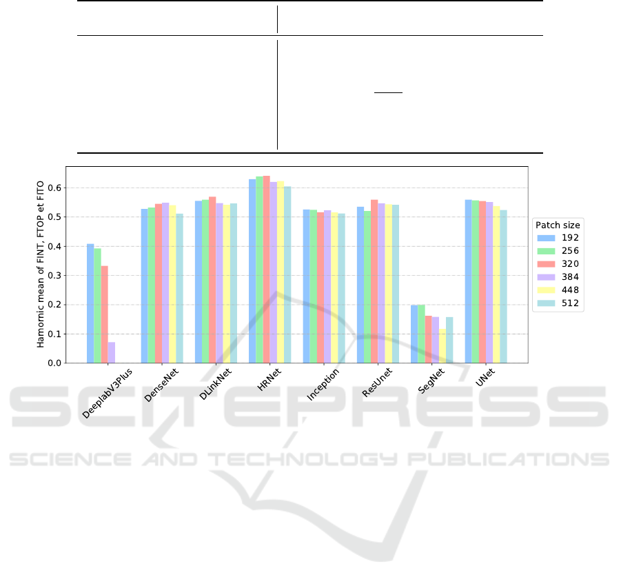
Table 4: Harmonic mean of FINT, FTOP and FITO scores for different patch sizes.

Architecture

Patch Size

192 256 320 384 448 512

DeeplabV3Plus (Chen et al., 2018) 0.408 0.392 0.333 0.072 0 0

DenseNet (Huang et al., 2017) 0.527 0.532 0.545 0.549 0.540 0.512

DLinkNet (Zhou et al., 2018) 0.555 0.559 0.569 0.547 0.542 0.546

HRNet (Wang et al., 2020) 0.629 0.639 0.641 0.620 0.623 0.605

Inception (Punn and Agarwal, 2020) 0.525 0.525 0.516 0.523 0.516 0.512

ResUnet (He et al., 2015) 0.535 0.521 0.559 0.547 0.543 0.542

SegNet (Badrinarayanan et al., 2017) 0.198 0.199 0.162 0.158 0.117 0.158

UNet (Ronneberger et al., 2015) 0.560 0.557 0.555 0.551 0.537 0.524

Figure 4: Comparative analysis of model performance across varying patch sizes, showing the harmonic mean of FINT, FTOP,

and FITO scores for different convolutional neural network architectures.

4 CONCLUSION

This study provides a contribution to the ﬁeld of au-

tomated map generation from GPS trajectory data,

focusing on hiking maps without relying on aerial

imagery. By evaluating several neural network ar-

chitectures, we identiﬁed HRNet as the most ef-

ﬁcient model for this task, especially when using

the heatmap data feature in isolation. Our ﬁndings

highlight the importance of feature selection, with

heatmaps offering superior results for mapping com-

plex trail networks. Although our approach was tested

on a speciﬁc dataset, its implications extend to vari-

ous geospatial applications that depend on GPS data

for accurate and up-to-date maps. Future work could

explore the integration of additional data types, as

well as reﬁning the architectures to improve perfor-

mance in other geographical contexts. Also, explor-

ing methods that directly process GPS data as spatio-

temporal information to eliminate the need for con-

verting vector data into raster data, could be highly

beneﬁcial. While several approaches exist in this do-

main, none have yet been applied to automatic map

inference from GPS data.

REFERENCES

Abdollahi, A., Pradhan, B., Shukla, N., Chakraborty, S.,

and Alamri, A. (2020). Deep learning approaches ap-

plied to remote sensing datasets for road extraction: A

state-of-the-art review. Remote Sensing, 12(9):1444.

Ahmed, M. and Wenk, C. (2012). Constructing street net-

works from gps trajectories. In Algorithms–ESA 2012:

20th Annual European Symposium, Ljubljana, Slove-

nia, September 10-12, 2012. Proceedings 20, pages

60–71. Springer.

Alsahﬁ, T. et al. (2020). Road map generation and feature

extraction algorithms from GPS trajectories and Tra-

jectories Data warehousing. PhD thesis, University of

Texas.

Badrinarayanan, V., Kendall, A., and Cipolla, R. (2017).

Segnet: A deep convolutional encoder-decoder ar-

chitecture for image segmentation. IEEE transac-

Deep Neural Network Architectures for Advanced Hiking Map Generation

539

Figure 5: Visual outcomes from the 3 ﬁrst training iterations per input combination employing the HRNet architecture and a

patch size of 320.

tions on pattern analysis and machine intelligence,

39(12):2481–2495.

Biagioni, J. and Eriksson, J. (2012a). Inferring road

maps from global positioning system traces: Survey

and comparative evaluation. Transportation research

record, 2291(1):61–71.

Biagioni, J. and Eriksson, J. (2012b). Map inference in the

face of noise and disparity. In Proceedings of the 20th

International Conference on Advances in Geographic

Information Systems, SIGSPATIAL ’12, page 79–88,

New York, NY, USA. Association for Computing Ma-

chinery.

Cao, L. and Krumm, J. (2009). From gps traces to a routable

road map. In 17th ACM SIGSPATIAL International

Conference on Advances in Geographic Information

Systems (ACM SIGSPATIAL GIS 2009), November 4-

6, 2009, Seattle, WA, pages 3–12.

Chao, P., Hua, W., Mao, R., Xu, J., and Zhou, X. (2020).

A survey and quantitative study on map inference al-

gorithms from gps trajectories. IEEE Transactions on

Knowledge and Data Engineering, 34(1):15–28.

Chen, L.-C., Zhu, Y., Papandreou, G., Schroff, F., and

Adam, H. (2018). Encoder-decoder with atrous sepa-

rable convolution for semantic image segmentation. In

Proceedings of the European conference on computer

vision (ECCV), pages 801–818.

Chen, Z., Xiao, X., Gong, Y.-J., Fang, J., Ma, N., Chai, H.,

and Cao, Z. (2022). Interpreting trajectories from mul-

tiple views: A hierarchical self-attention network for

estimating the time of arrival. In Proceedings of the

28th ACM SIGKDD Conference on Knowledge Dis-

covery and Data Mining, pages 2771–2779.

Dal Poz, A., Martins, E., and Zanin, R. (2022). Road net-

work extraction using gps trajectories based on mor-

phological and skeletonization algorithms. The In-

ternational Archives of the Photogrammetry, Remote

Sensing and Spatial Information Sciences, 43:239–

245.

Eftelioglu, E., Garg, R., Kango, V., Gohil, C., and Chowd-

hury, A. R. (2022). Ring-net: road inference from

gps trajectories using a deep segmentation network.

In Proceedings of the 10th ACM SIGSPATIAL Inter-

national Workshop on Analytics for Big Geospatial

Data, pages 17–26.

Feng, S., Chen, L., Xiong, W., and Deng, Y. (2020). A

method of extracting road network structure from tra-

jectory data based on u-net network. In 2020 IEEE

International Conference on Information Technology,

Big Data and Artiﬁcial Intelligence (ICIBA), vol-

ume 1, pages 1388–1392. IEEE.

Fu, Z., Fan, L., Sun, Y., and Tian, Z. (2020). Density adap-

tive approach for generating road network from gps

trajectories. IEEE Access, 8:51388–51399.

Guo, Y., Bardera, A., Fort, M., and Silveira, R. I. (2021). A

scalable method to construct compact road networks

from gps trajectories. International Journal of Geo-

graphical Information Science, 35(7):1309–1345.

Guo, Y., Li, B., Lu, Z., and Zhou, J. (2022). A novel method

for road network mining from ﬂoating car data. Geo-

spatial Information Science, 25(2):197–211.

He, K., Zhang, X., Ren, S., and Sun, J. (2015). Deep

residual learning for image recognition. CoRR,

abs/1512.03385.

He, S., Bastani, F., Abbar, S., Alizadeh, M., Balakrishnan,

ICPRAM 2025 - 14th International Conference on Pattern Recognition Applications and Methods

540

H., Chawla, S., and Madden, S. (2018). Roadrun-

ner: improving the precision of road network infer-

ence from gps trajectories. In Proceedings of the 26th

ACM SIGSPATIAL International Conference on Ad-

vances in Geographic Information Systems, pages 3–

12.

He, T., Bao, J., Li, R., Ruan, S., Li, Y., Song, L., He, H.,

and Zheng, Y. (2020). What is the human mobility in

a new city: Transfer mobility knowledge across cities.

In Proceedings of The Web Conference 2020, WWW

’20, page 1355–1365, New York, NY, USA. Associa-

tion for Computing Machinery.

Huang, G., Liu, Z., Van Der Maaten, L., and Weinberger,

K. Q. (2017). Densely connected convolutional net-

works. In Proceedings of the IEEE conference on

computer vision and pattern recognition, pages 4700–

4708.

Karagiorgou, S. and Pfoser, D. (2012). On vehicle tracking

data-based road network generation. In Proceedings

of the 20th International Conference on Advances in

Geographic Information Systems, pages 89–98.

Li, M., Tong, P., Li, M., Jin, Z., Huang, J., and Hua, X.-S.

(2021). Trafﬁc ﬂow prediction with vehicle trajecto-

ries. In Proceedings of the AAAI Conference on Arti-

ﬁcial Intelligence, volume 35, pages 294–302.

Liu, L., Yang, Z., Li, G., Wang, K., Chen, T., and Lin, L.

(2022). Aerial images meet crowdsourced trajectories:

a new approach to robust road extraction. IEEE trans-

actions on neural networks and learning systems.

Prabowo, A., Koniusz, P., Shao, W., and Salim, F. D.

(2019). Coltrane: Convolutional trajectory network

for deep map inference. In Proceedings of the

6th ACM International Conference on Systems for

Energy-Efﬁcient Buildings, Cities, and Transporta-

tion, pages 21–30.

Punn, N. S. and Agarwal, S. (2020). Inception u-net ar-

chitecture for semantic segmentation to identify nu-

clei in microscopy cell images. ACM Transactions on

Multimedia Computing, Communications, and Appli-

cations (TOMM), 16(1):1–15.

Ronneberger, O., Fischer, P., and Brox, T. (2015). U-net:

Convolutional networks for biomedical image seg-

mentation. CoRR, abs/1505.04597.

Roy, A., Lanco Bertrand, S., and Fablet, R. (2022). Deep

inference of seabird dives from gps-only records: Per-

formance and generalization properties. PLoS Com-

putational Biology, 18(3):e1009890.

Ruan, S., Bao, J., Liang, Y., Li, R., He, T., Meng, C., Li,

Y., Wu, Y., and Zheng, Y. (2020a). Dynamic public

resource allocation based on human mobility predic-

tion. Proceedings of the ACM on interactive, mobile,

wearable and ubiquitous technologies, 4(1):1–22.

Ruan, S., Long, C., Bao, J., Li, C., Yu, Z., Li, R., Liang, Y.,

He, T., and Zheng, Y. (2020b). Learning to generate

maps from trajectories. Proceedings of the AAAI Con-

ference on Artiﬁcial Intelligence, 34(01):890–897.

Stanojevic, R., Abbar, S., Thirumuruganathan, S., Chawla,

S., Filali, F., and Aleimat, A. (2018). Robust road

map inference through network alignment of trajecto-

ries. In Proceedings of the 2018 SIAM International

Conference on Data Mining, pages 135–143. SIAM.

Sun, T., Di, Z., Che, P., Liu, C., and Wang, Y. (2019). Lever-

aging crowdsourced gps data for road extraction from

aerial imagery. In Proceedings of the IEEE/CVF Con-

ference on Computer Vision and Pattern Recognition,

pages 7509–7518.

Tveite, H. (2015–2019). The QGIS thin greyscale im-

age to skeleton plugin. http://plugins.qgis.org/plugins/

ThinGreyscale/.

Wang, J., Sun, K., Cheng, T., Jiang, B., Deng, C., Zhao,

Y., Liu, D., Mu, Y., Tan, M., Wang, X., et al. (2020).

Deep high-resolution representation learning for vi-

sual recognition. IEEE transactions on pattern analy-

sis and machine intelligence, 43(10):3349–3364.

Wu, H., Zhang, H., Zhang, X., Sun, W., Zheng, B., and

Jiang, Y. (2020). Deepdualmapper: A gated fusion

network for automatic map extraction using aerial im-

ages and trajectories. In Proceedings of the AAAI Con-

ference on Artiﬁcial Intelligence, volume 34, pages

1037–1045.

Yang, X., Tang, L., Ren, C., Chen, Y., Xie, Z., and Li,

Q. (2020). Pedestrian network generation based on

crowdsourced tracking data. International Journal of

Geographical Information Science, 34(5):1051–1074.

Zhang, C., Li, Y., Xiang, L., Jiao, F., Wu, C., and Li,

S. (2021). Generating road networks for old down-

town areas based on crowd-sourced vehicle trajecto-

ries. Sensors, 21(1):235.

Zhang, J., Hu, Q., Li, J., and Ai, M. (2020). Learning

from gps trajectories of ﬂoating car for cnn-based ur-

ban road extraction with high-resolution satellite im-

agery. IEEE Transactions on Geoscience and Remote

Sensing, 59(3):1836–1847.

Zheng, R., Liu, Q., Rao, W., Yuan, M., Zeng, J., and Jin,

Z. (2017). Topic model-based road network infer-

ence from massive trajectories. In 2017 18th IEEE In-

ternational Conference on Mobile Data Management

(MDM), pages 246–255. IEEE.

Zhou, L., Zhang, C., and Wu, M. (2018). D-linknet: Linknet

with pretrained encoder and dilated convolution for

high resolution satellite imagery road extraction. In

Proceedings of the IEEE Conference on Computer Vi-

sion and Pattern Recognition Workshops, pages 182–

186.

Zhou, Y., Wang, J., and Zhan, Y. (2022). An urban road

extraction method based on trajectory clustering. In

IGARSS 2022-2022 IEEE International Geoscience

and Remote Sensing Symposium, pages 1268–1271.

IEEE.

Zhu, Q., Zhang, Y., Wang, L., Zhong, Y., Guan, Q., Lu,

X., Zhang, L., and Li, D. (2021). A global context-

aware and batch-independent network for road extrac-

tion from vhr satellite imagery. ISPRS Journal of Pho-

togrammetry and Remote Sensing, 175:353–365.

Deep Neural Network Architectures for Advanced Hiking Map Generation

541