Breast Cancer Image Classification Using Deep Learning and Test-Time
Augmentation
Jo
˜
ao Fernando Mari
1
, Larissa Ferreira Rodrigues Moreira
1
, Leandro Henrique Furtado Pinto Silva
1
,
Mauricio C. Escarpinati
2
and Andr
´
e R. Backes
3
1
Institute of Exact and Technological Sciences, Federal University of Vic¸osa - UFV, Rio Parana
´
ıba-MG, Brazil
2
School of Computer Science, Federal University of Uberl
ˆ
andia, Uberl
ˆ
andia-MG, Brazil
3
Department of Computing, Federal University of S
˜
ao Carlos, S
˜
ao Carlos-SP, Brazil
Keywords:
Breast Cancer, Deep Learning, Test-Time Augmentation, Image Classification.
Abstract:
Deep learning-based computer vision methods can improve diagnostic accuracy, efficiency, and productivity.
While traditional approaches primarily apply Data Augmentation (DA) during the training phase, Test-Time
Augmentation (TTA) offers a complementary strategy to improve the predictive capabilities of trained models
without increasing training time. In this study, we propose a simple and effective TTA strategy to enhance the
classification of histopathological images of breast cancer. After optimizing hyperparameters, we evaluated the
TTA strategy across all magnifications of the BreakHis dataset using three deep learning architectures, trained
with and without DA. We compared five sets of transformations and multiple prediction rounds. The proposed
strategy significantly improved the mean accuracy across all magnifications, demonstrating its effectiveness in
improving model performance.
1 INTRODUCTION
Histopathological image classification plays a crucial
role in diagnosing breast cancer. Pathologists an-
alyze microscopic slides of breast tissue at various
magnifications to identify tumor characteristics, such
as determining whether a tumor is benign or malig-
nant. However, manual analysis is often subjective,
time-consuming, and prone to variability among ex-
perts. To address these limitations, computer vision
and deep learning techniques have been increasingly
adopted, offering improved diagnostic accuracy and
efficiency (Gautam, 2023).
Traditional deep learning methods for image
classification commonly employ data augmentation
(DA) during training to enhance model generaliza-
tion (da Silva et al., 2020; Gautam, 2023; Barbosa
et al., 2024). Although DA is effective, it does not
leverage the potential of augmentations during the
testing phase. Test-Time Augmentation (TTA) ex-
tends the application of data transformations to in-
ference, enhancing the model’s predictions without
incurring additional training costs (Calvo-Zaragoza
et al., 2020; Shanmugam et al., 2021; Valero-Mas
et al., 2024). Previous research has shown the benefits
of TTA in various medical imaging tasks, including
skin cancer classification and bone fracture detection,
demonstrating its ability to improve predictive accu-
racy in different datasets and architectures (Shorten
and Khoshgoftaar, 2019; Garcea et al., 2023).
Despite its proven effectiveness, TTA has only
been minimally explored in the context of histopatho-
logical image classification of breast cancer. Most
studies focus on specific magnification levels or mod-
els, neglecting a broader evaluation across magnifica-
tions and architectures (Gupta et al., 2021; Oza et al.,
2024). This leaves a significant gap in understand-
ing TTA’s potential in multi-resolution medical imag-
ing scenarios, such as the BreakHis dataset (Spanhol
et al., 2016).
In this paper, we propose a simple and effec-
tive TTA strategy to improve the classification of
histopathological images of breast cancer. Using
the BreakHis dataset, we evaluate TTA across all
magnification levels and analyze its impact on three
deep learning architectures: ResNet-50, Vision Trans-
former (ViT), and Swin Transformer V2. Our study
also compares the effects of training-time DA on the
performance of TTA.
The main contributions of this work are: (i) a
Mari, J. F., Moreira, L. F. R., Silva, L. H. F. P., Escarpinati, M. C. and Backes, A. R.
Breast Cancer Image Classification Using Deep Learning and Test-Time Augmentation.
DOI: 10.5220/0013359200003912
Paper published under CC license (CC BY-NC-ND 4.0)
In Proceedings of the 20th International Joint Conference on Computer Vision, Imaging and Computer Graphics Theory and Applications (VISIGRAPP 2025) - Volume 3: VISAPP, pages
761-768
ISBN: 978-989-758-728-3; ISSN: 2184-4321
Proceedings Copyright © 2025 by SCITEPRESS – Science and Technology Publications, Lda.
761

comprehensive evaluation of TTA across four mag-
nification levels (40×, 100×, 200×, and 400×) in
the BreakHis dataset, (ii) analysis of TTA’s impact
on three deep learning architectures trained both with
and without DA, (iii) identify the best transforma-
tion sets for TTA in breast cancer image classifica-
tion, and (iv) demonstrates TTA’s ability to improve
model generalization and accuracy under diverse test-
ing conditions.
The remainder of this paper is organized as fol-
lows. Section 2 reviews related work. We detail the
materials and methods used in Section 3. Section
4 presents the experimental design while Section 5
presents and discusses the results obtained. Finally,
Section 6 concludes with future research directions.
2 RELATED WORK
Nguyen et al. (2019) developed an approach to breast
cancer classification using weighted feature selection
with a Convolutional Neural Network (CNN) clas-
sifier, incorporating Test-Time Augmentation (TTA)
strategy involved transforming test images with hori-
zontal and vertical flips and 90
◦
rotations to improve
classification accuracy. Gupta et al. (2021) proposed
a modified ResNet to classify images as benign or
malignant on the BreakHis dataset by incorporating
TTA. However, their Residual network was trained
exclusively using 40× magnification images.
Kandel and Castelli (2021) investigated the im-
pact of TTA on X-ray images for bone fracture detec-
tion using five CNN architectures and the combina-
tion of different Data Augmentation (DA) techniques
based on rotation, flips, and zoom. In Nanni et al.
(2021) authors evaluated different datasets, including
virus textures, and explored the effectiveness of vari-
ous DA techniques such as kernel filters, color space
transformations, geometric transformations, random
erasing/cutting, and image mixing.
Jiahao et al. (2021) proposed a method based on
the EfficientNet architecture to identify skin cancer
in dermoscopy images by leveraging DA strategies
during training and Test-Time Augmentation during
inference to improve classification accuracy. In the
same application context, Goceri (2023) applied TTA
to identify skin cancer and evaluated three CNN ar-
chitectures: DenseNet, ResNet, and VGG.
M
¨
uller et al. (2022) evaluated the use of TTA
on different medical imaging datasets, including
histopathological images of colorectal cancer. More-
over, they tested different CNN architectures and ob-
served that TTA is a promising technique that does
not require additional training time.
Oza et al. (2024) investigated the use of deep
learning to diagnose breast cancer from mammo-
grams with abnormal lesions, using a transfer learning
strategy and TTA to enhance the classification perfor-
mance. They evaluated four pre-trained CNN models
and exploited DA based on rotation with various an-
gles: horizontal flip, zoom, and shearing.
Unlike the aforementioned studies, to the best of
our knowledge, this is the first study to explore TTA
across all magnifications of the BreakHis dataset. We
used modern deep learning architectures, including
ResNet-50, ViT-16, and Swin Transformer V2, en-
hanced by hyperparameter optimization. Moreover,
TTA enhances the capability of the model to adapt
to various testing conditions, ensuring a more re-
liable assessment of breast cancer classification in
histopathological images across different image mag-
nifications.
3 MATERIAL AND METHODS
3.1 Dataset
We used the BreakHis dataset
1
(Spanhol et al., 2016,
2017), a well-established benchmark for breast cancer
histopathological image classification. The dataset
comprises 7,909 microscopic images of breast tumor
tissue collected from 82 patients. These images are
captured at four magnification levels: 40×, 100×,
200×, and 400×. Each image is labeled benign or
malignant, with 2,480 images in the benign class and
5,429 in the malignant class. This diversity in magni-
fication levels allows us to evaluate the classification
models under varying resolutions, a common scenario
in histopathological analysis. Dataset includes five
predefined random folds to ensure robust evaluation.
Each fold features a patient-wise split, where all im-
ages from a single patient are allocated exclusively to
the training or test sets. This approach avoids over-
lap and ensures the models are tested on unseen data,
replicating real-world scenarios where generalization
to new patients is critical.
3.2 Architectures
We selected three deep learning architectures to eval-
uate our approaches: ResNet-50 (He et al., 2016), ViT
b16 (Dosovitskiy et al., 2021), and Swin Transformer
V2 (Liu et al., 2022). These architectures are widely
1
https://web.inf.ufpr.br/vri/databases/breast-cancer-
histopathological-database-breakhis/
VISAPP 2025 - 20th International Conference on Computer Vision Theory and Applications
762

recognized for their high performance in tasks related
to image classification and object detection.
ResNet-50 introduced residual learning, enabling
the training of deeper networks than earlier CNNs.
This architecture mitigates the vanishing gradient
problem using residual blocks comprising convolu-
tional layers and skip connections. Skip connections
bypass one or more residual blocks, allowing the net-
work to learn identity mappings and enhancing gradi-
ent flow during backpropagation (He et al., 2016).
ViT b16 (Vision Transformer) leverages a
Transformer-based architecture originally designed
for natural language processing and adapts it to com-
puter vision tasks. Proposed by Dosovitskiy et al.
(2021), ViT divides input images into fixed-size
patches, treating each patch as a token. These tokens
are processed through a series of self-attention mech-
anisms to learn embeddings, enabling the model to
capture global relationships across the image.
Swin Transformer V2, introduced by Liu et al.
(2022), enhances the Swin Transformer with a hier-
archical architecture that uses windowing for local
attention and improves the computational efficiency
over ViT’s global attention. By processing smaller
image windows and shifting them across layers, it ef-
fectively captures both the local and global contexts,
making it highly suitable for image classification.
4 EXPERIMENT DESIGN
In this study, we designed experiments to evaluate
the effectiveness of TTA strategies for histopatho-
logical image classification of breast cancer using
the BreakHis dataset (Section 3.1). The dataset is
provided with five randomized folds, already split
patient-wise into training and test sets. For each fold,
we further split 20% of the training set, on an image-
wise basis, to construct a validation set.
The validation set served two purposes: hyper-
parameter optimization and early stopping. Hyper-
parameter optimization focused on selecting the best
values for batch size (BS) and learning rate (LR). A
grid search approach was used, exploring BS values
of 16, 32, 64, 128 and LR values of 0.01, 0.001,
0.0001, 0.00001. To reduce computational demands,
hyperparameter optimization was conducted only on
the first fold using images with a magnification of
40× for each architecture. The best-performing hy-
perparameters were then applied to all folds and mag-
nifications.
The Adam optimizer and cross-entropy loss func-
tion were used to fine-tune models pre-trained on the
ImageNet dataset (Deng et al., 2009). All layers of the
models were unfrozen during training to enable fine-
tuning. A learning rate scheduler was implemented to
reduce the learning rate if the validation loss did not
improve after ten consecutive epochs (reduce LR on
plateau). An early stopping strategy was also applied,
halting training if the validation loss failed to improve
after 21 epochs.
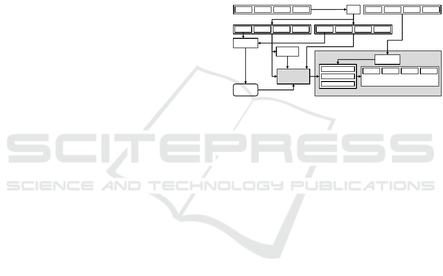
Figure 1 illustrates the experimental design, which
includes the steps of data splitting, hyperparameter
optimization, model training with and without data
augmentation, and prediction using the TTA strategy.
This systematic approach ensures the reliable evalua-
tion of TTA’s impact on classification performance.
ResNet-50
ViT b16
Swin T V2 base
40x 100x 200x 400x
40x 100x 200x 400x
40x 100x 200x 400x 40x 100x 200x 400x
SPLIT
HP
optimization
Model
training
HP
Test DA
Original training dataset (5 folds)
Training
DA
Training dataset Validation dataset
Original test dataset (5 folds)
Repeat for N rounds
N = {1, 5, 9, 15, 25}
Training
with DA
Training
without DA
Prediction
(Most frequent class among the N rounds)
40x 100x 200x 400x
Used for early
stopping
Only for
fold 1,
and 40x
Mean over the 5 folds
TEST-TIME
AUGMENTATION
MODELS
(a)
(b)
(c)
(d)
Figure 1: The experiment design illustration. (a) We split
the training set to create a validation set. (b) Hyperparame-
ter optimization. (c) Training the models with and without
DA. (d) Prediction with the proposed TTA strategy.
4.1 Training-Time Data Augmentation
We trained one model for each architecture, magni-
fication, and fold, following the hyperparameter op-
timization and training strategies outlined in Section
4. This training was conducted with and without a
DA strategy. Three different transformation pipelines
were used for the datasets: T-1 was applied to the vali-
dation and test sets, T-2 was applied to the training set
for models trained without DA, and T-3 was applied
to the training set for models trained with DA.
In all cases, the images were normalized using the
mean and standard deviation of the ImageNet dataset
to ensure compatibility with pre-trained models. The
transformations are detailed as follows: T-1: The im-
ages were resized to 256×256 pixels, followed by a
center crop to 224×224 pixels. T-2: Random re-
sized cropping with patches covering between 80%-
100% of the original image size. T-3: A sequence
of augmentations including: Random horizontal flip-
ping. Random rotation between -15
◦
and 15
◦
. Ran-
dom resized cropping with patches covering 80% to
100% of the original image size. Color jittering, with
brightness, contrast, and saturation adjusted by a fac-
tor randomly chosen between 0.8 and 1.2. Random
erasing, with patches covering 2% to 20% of the orig-
inal image size. These transformations were carefully
Breast Cancer Image Classification Using Deep Learning and Test-Time Augmentation
763

selected to enhance the models’ generalization capa-
bilities, particularly when using DA, and to provide a
consistent testing baseline for fair comparison.
4.2 Test-Time Augmentation (TTA)
In this work, we propose a simple but effective TTA
strategy to enhance the accuracy of classification
models with minimal computational overhead. The
approach involves making multiple predictions for
each test image by applying a DA strategy to generate
augmented versions of the image. The final prediction
is determined using a majority voting mechanism, as
defined by Equation 1.
ˆy =
(
1, if
∑
N
i=1
f (T(x)) >
N
2
,
0, otherwise
(1)
where ˆy is the final prediction label, N denotes the
number of TTA prediction rounds, and T (x) refers to
the transformation set applied to the test image x. The
function f represents the deep learning model used
to predict the output for the transformed image T (x).
The term
∑
N
i=1
f (T(x)) is the sum of the binary pre-
dictions (0 or 1) for each transformed image, and
N
2
serves as the decision threshold. If the sum is greater
than
N
2
, more than half of the predictions are 1, and the
final prediction ˆy is set to 1; otherwise, ˆy is set to 0.
This majority voting strategy aggregates predictions
from multiple augmented versions of the test image
to improve robustness.
We evaluated five transformation sets for TTA
during the prediction phase: T-A: Random resized
crop with patches between 80% and 100% of the
original image size. T-B: Random resized crop with
patches between 50% and 100% of the original image
size. T-C: Random horizontal flip, followed by ran-
dom rotation (-15
◦
to 15
◦
), and a random resized crop
with patches between 80% and 100% of the original
size. T-D: Random horizontal flip, followed by ran-
dom rotation (-15
◦
to 15
◦
), and a random resized crop
with patches between 50% and 100% of the original
size. T-E: Identical to the transformation set T-3 de-
scribed in Section 4.1, combining random horizontal
flip, random rotation, random resized crop, color jit-
tering, and random erasing. This TTA strategy lever-
ages multiple augmentations to reduce prediction un-
certainties and improve the robustness of the model
by considering diverse perspectives of the same input
image.
5 RESULTS AND DISCUSSION
For the experiments we used a PC running Linux
Ubuntu 22.04 LTS, equipped with a Core I5-12400
with 6 cores, up to 4.40 GHz CPU, 32 GB of RAM,
and a GPU NVIDIA RTX 4090 with 24 GB of mem-
ory. The experiments were developed using Python
3.10, PyTorch 2.2.2, torchvision 0.17.2 with CUDA
Toolkit 10.1, and Scikit-learn 1.4.2. The pre-trained
models were obtained from the torchvision library.
To evaluate the performance of our method, we
used the accuracy, which measures the proportion of
correctly classified samples out of the total number of
samples, providing a straightforward metric to evalu-
ate the overall effectiveness of the models in classify-
ing histopathological images.
Table 1 presents the results of the hyperparame-
ter optimization described in Section 4. Each row
lists the BS and LR that achieved the highest valida-
tion accuracy for the respective architecture. We also
included the number of epochs required before early
stopping was triggered. These optimized BS and LR
values were consistently applied to train all models in
this study.
Table 1: Optimized hyperparameter values for each archi-
tecture.
Architecture BS LR Acc. Val. Epochs
ResNet-50 32 0.0001 0.9820 14
ViT b16 64 0.0001 0.9910 28
Swin T. V2 base 16 0.0001 0.9930 9
Table 2 presents the test accuracy for models
trained with and without DA. Since the BreakHis
dataset consists of five folds, the reported values rep-
resent the mean accuracy across these folds. The re-
sults demonstrate that applying DA during training
improves the test accuracy using the standard predic-
tion strategy, i.e., without employing TTA. Bold val-
ues indicate the highest accuracy achieved for each
magnification level and architecture. The values in
this table provide the baseline for evaluating the TTA
strategies.
Table 2: Test accuracy obtained with the standard test strat-
egy with models trained with and without DA.
ResNet-50 ViT b16 Swin T. V2 base
Mag. No DA DA No DA DA No DA DA
40× 0.8483 0.8798 0.8394 0.8582 0.8883 0.8963
100× 0.8578 0.8750 0.8298 0.8525 0.8929 0.8785
200× 0.8692 0.8866 0.8724 0.8825 0.8913 0.8979
400× 0.8170 0.8679 0.8167 0.8426 0.8558 0.8608
Mean: 0.8481 0.8773 0.8396 0.8590 0.8821 0.8834
Tables 3 and 4 summarize the mean accuracy
across all magnifications (40×, 100×, 200×, and
400×) achieved using the TTA strategy for each trans-
formation set (T-A, T-B, T-C, T-D, and T-E) with 1, 5,
VISAPP 2025 - 20th International Conference on Computer Vision Theory and Applications
764

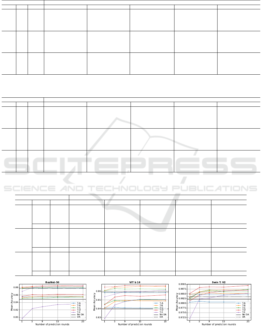
Table 3: The test accuracy obtained through the TTA strategy with 1, 5, 6, 15, and 25 rounds of predictions considering five
different transformation sets (TS) with the models trained without DA (No DA).
Accuracy (Improvement over No DA) [t-value]
Arch. TS No DA 1 5 9 15 25
ResNet-50
T-A 0.8481 0.8548 (+0.0067) [3.57] 0.8551 (+0.0070) [3.07] 0.8549 (+0.0068) [3.06] 0.8551 (+0.0070) [3.16] 0.8551 (+0.0070) [3.16]
T-B 0.8481 0.8523 (+0.0042) [3.33] 0.8554 (+0.0073) [7.46] 0.8561 (+0.0080) [10.01] 0.8567 (+0.0086) [7.38] 0.8554 (+0.0073) [8.33]
T-C 0.8481 0.8507 (+0.0026) [0.57] 0.8519 (+0.0038) [0.91] 0.8515 (+0.0034) [0.80] 0.8534 (+0.0053) [1.14] 0.8542 (+0.0061) [1.50]
T-D 0.8481 0.8563 (+0.0082) [2.85] 0.8607 (+0.0126) [6.56] 0.8601 (+0.0120) [9.56] 0.8616 (+0.0136) [8.52] 0.8610 (+0.0129) [9.38]
T-E 0.8481 0.7969 (-0.0512) [-5.92] 0.8235 (-0.0246) [-4.30] 0.8283 (-0.0198) [-3.63] 0.8342 (-0.0139) [-3.70] 0.8360 (-0.0121) [-2.43]
ViT b16
T-A 0.8396 0.8414 (+0.0019) [0.67] 0.8415 (+0.0019) [0.63] 0.8409 (+0.0014) [0.47] 0.8408 (+0.0012) [0.41] 0.8406 (+0.0010) [0.36]
T-B 0.8396 0.8406 (+0.0011) [0.45] 0.8480 (+0.0085) [6.18] 0.8494 (+0.0098) [5.92] 0.8490 (+0.0095) [6.39] 0.8489 (+0.0093) [8.23]
T-C 0.8396 0.8451 (+0.0056) [1.27] 0.8494 (+0.0098) [2.82] 0.8484 (+0.0088) [2.65] 0.8503 (+0.0108) [3.29] 0.8503 (+0.0108) [2.81]
T-D 0.8396 0.8445 (+0.0049) [1.24] 0.8532 (+0.0136) [3.35] 0.8549 (+0.0153) [3.48] 0.8541 (+0.0146) [3.05] 0.8556 (+0.0160) [3.38]
T-E 0.8396 0.8288 (-0.0108) [-1.58] 0.8442 (+0.0046) [1.16] 0.8481 (+0.0085) [2.69] 0.8507 (+0.0112) [4.72] 0.8504 (+0.0109) [3.59]
Swin T. V2
base
T-A 0.8821 0.8805 (-0.0016) [-0.43] 0.8810 (-0.0010) [-0.29] 0.8806 (-0.0014) [-0.38] 0.8806 (-0.0014) [-0.39] 0.8806 (-0.0014) [-0.39]
T-B 0.8821 0.8813 (-0.0008) [-0.49] 0.8845 (+0.0025) [1.40] 0.8855 (+0.0034) [2.29] 0.8850 (+0.0029) [2.34] 0.8852 (+0.0031) [1.87]
T-C 0.8821 0.8822 (+0.0001) [0.04] 0.8860 (+0.0039) [1.27] 0.8870 (+0.0050) [1.35] 0.8863 (+0.0043) [1.52] 0.8873 (+0.0052) [1.95]
T-D 0.8821 0.8851 (+0.0031) [1.75] 0.8883 (+0.0063) [5.21] 0.8886 (+0.0066) [2.86] 0.8885 (+0.0064) [2.69] 0.8893 (+0.0072) [3.51]
T-E 0.8821 0.8719 (-0.0101) [-2.11] 0.8822 (+0.0002) [0.04] 0.8827 (+0.0006) [0.15] 0.8842 (+0.0021) [0.53] 0.8852 (+0.0032) [0.97]
Table 4: The test accuracy obtained through the TTA strategy with 1, 5, 6, 15, and 25 rounds of predictions considering five
different transformation sets (TS) with the models trained with DA.
Mean accuracy (Improvement over DA) [t-value]
Arch. TS DA 1 5 9 15 25
ResNet-50
T-A 0.8773 0.8792 (+0.0019) [0.45] 0.8787 (+0.0013) [0.34] 0.8786 (+0.0013) [0.32] 0.8785 (+0.0012) [0.29] 0.8785 (+0.0012) [0.29]
T-B 0.8773 0.8793 (+0.0020) [0.99] 0.8813 (+0.0039) [1.29] 0.8818 (+0.0045) [1.34] 0.8832 (+0.0058) [2.25] 0.8827 (+0.0054) [1.95]
T-C 0.8773 0.8778 (+0.0004) [0.10] 0.8791 (+0.0017) [0.46] 0.8798 (+0.0024) [0.64] 0.8809 (+0.0036) [0.84] 0.8805 (+0.0031) [0.73]
T-D 0.8773 0.8811 (+0.0038) [1.60] 0.8828 (+0.0055) [1.79] 0.8844 (+0.0070) [2.25] 0.8851 (+0.0077) [2.54] 0.8847 (+0.0074) [2.39]
T-E 0.8773 0.8694 (-0.0079) [-2.11] 0.8799 (+0.0026) [0.59] 0.8828 (+0.0054) [1.25] 0.8827 (+0.0054) [1.29] 0.8834 (+0.0061) [1.39]
ViT b16
T-A 0.8590 0.8581 (-0.0008) [-0.29] 0.8583 (-0.0006) [-0.24] 0.8583 (-0.0007) [-0.25] 0.8581 (-0.0009) [-0.33] 0.8581 (-0.0009) [-0.34]
T-B 0.8590 0.8606 (+0.0017) [0.86] 0.8646 (+0.0056) [2.48] 0.8644 (+0.0054) [2.41] 0.8656 (+0.0066) [2.26] 0.8650 (+0.0060) [1.94]
T-C 0.8590 0.8602 (+0.0012) [0.60] 0.8629 (+0.0040) [2.73] 0.8623 (+0.0033) [2.17] 0.8625 (+0.0035) [2.02] 0.8622 (+0.0032) [1.87]
T-D 0.8590 0.8646 (+0.0057) [1.93] 0.8650 (+0.0061) [3.04] 0.8663 (+0.0073) [3.49] 0.8660 (+0.0070) [3.37] 0.8659 (+0.0070) [4.36]
T-E 0.8590 0.8535 (-0.0055) [-1.81] 0.8565 (-0.0025) [-0.77] 0.8595 (+0.0005) [0.21] 0.8592 (+0.0002) [0.11] 0.8611 (+0.0022) [0.84]
Swin T. V2
base
T-A 0.8834 0.8846 (+0.0013) [0.40] 0.8845 (+0.0011) [0.36] 0.8844 (+0.0010) [0.31] 0.8844 (+0.0010) [0.31] 0.8844 (+0.0010) [0.31]
T-B 0.8834 0.8844 (+0.0011) [0.95] 0.8860 (+0.0027) [1.41] 0.8868 (+0.0034) [2.41] 0.8871 (+0.0037) [2.66] 0.8869 (+0.0036) [2.58]
T-C 0.8834 0.8831 (-0.0003) [-0.08] 0.8857 (+0.0023) [0.50] 0.8864 (+0.0030) [0.76] 0.8859 (+0.0025) [0.67] 0.8860 (+0.0026) [0.74]
T-D 0.8834 0.8829 (-0.0005) [-0.16] 0.8858 (+0.0024) [1.26] 0.8858 (+0.0024) [1.38] 0.8864 (+0.0031) [2.14] 0.8868 (+0.0035) [2.53]
T-E 0.8834 0.8812 (-0.0022) [-0.83] 0.8841 (+0.0007) [0.16] 0.8852 (+0.0018) [0.51] 0.8866 (+0.0032) [1.02] 0.8868 (+0.0035) [1.07]
Table 5: The test accuracy obtained through the DA in the prediction with 1, 5, 6, 15, and 25 rounds of predictions considering
the transformation set T-D with the models trained without DA.
Accuracy when using transformation set T-D (Improvement over No DA)
Arch. Mag. No DA 1 5 9 15 25
ResNet-50
(T-D)
40× 0.8483 0.8627 (+0.0144) 0.8671 (+0.0189) 0.8641 (+0.0158) 0.8664 (+0.0182) 0.8648 (+0.0165)
100× 0.8578 0.8704 (+0.0126) 0.8699 (+0.0120) 0.8700 (+0.0122) 0.8726 (+0.0148) 0.8722 (+0.0143)
200× 0.8692 0.8690 (-0.0002) 0.8776 (+0.0084) 0.8802 (+0.0110) 0.8794 (+0.0101) 0.8785 (+0.0092)
400× 0.8170 0.8231 (+0.0061) 0.8282 (+0.0112) 0.8259 (+0.0089) 0.8281 (+0.0111) 0.8285 (+0.0115)
Mean: 0.8481 0.8563 (+0.0082) 0.8607 (+0.0126) 0.8601 (+0.0120) 0.8616 (+0.0136) 0.8610 (+0.0129)
ViT b16
(T-D)
40× 0.8394 0.8341 (-0.0053) 0.8422 (+0.0028) 0.8417 (+0.0023) 0.8407 (+0.0013) 0.8412 (+0.0018)
100× 0.8298 0.8467 (+0.0170) 0.8551 (+0.0253) 0.8568 (+0.0270) 0.8575 (+0.0278) 0.8581 (+0.0283)
200× 0.8724 0.8754 (+0.0030) 0.8835 (+0.0111) 0.8873 (+0.0149) 0.8842 (+0.0118) 0.8884 (+0.0160)
400× 0.8167 0.8216 (+0.0050) 0.8319 (+0.0153) 0.8338 (+0.0171) 0.8341 (+0.0174) 0.8346 (+0.0179)
Mean: 0.8396 0.8445 (+0.0049) 0.8532 (+0.0136) 0.8549 (+0.0153) 0.8541 (+0.0146) 0.8556 (+0.0160)
Swin T. V2
base (T-D)
40× 0.8883 0.8969 (+0.0086) 0.8987 (+0.0104) 0.9021 (+0.0137) 0.9028 (+0.0145) 0.9023 (+0.0139)
100× 0.8929 0.8964 (+0.0035) 0.8980 (+0.0052) 0.9002 (+0.0074) 0.8980 (+0.0051) 0.8996 (+0.0068)
200× 0.8913 0.8920 (+0.0007) 0.8966 (+0.0053) 0.8937 (+0.0024) 0.8941 (+0.0029) 0.8943 (+0.0031)
400× 0.8558 0.8552 (-0.0006) 0.8600 (+0.0042) 0.8585 (+0.0027) 0.8589 (+0.0031) 0.8608 (+0.0050)
Mean: 0.8821 0.8851 (+0.0031) 0.8883 (+0.0063) 0.8886 (+0.0066) 0.8885 (+0.0064) 0.8893 (+0.0072)
Figure 2: Line charts illustrating the mean test accuracy achieved using the TTA strategy with 1, 5, 9, and 25 prediction
rounds, evaluated across the five transformation strategies applied to models trained without DA (solid lines) and with DA
(dashed lines).
Breast Cancer Image Classification Using Deep Learning and Test-Time Augmentation
765

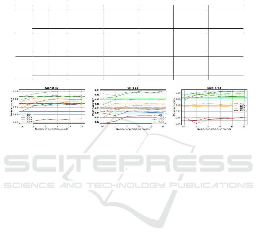
Table 6: The test accuracy obtained through the Test-Time Augmentation with 1, 5, 6, 15, and 25 rounds of predictions
considering the best transformation set with the models trained with DA.
Accuracy when using the best transformation set (Improvement over DA)
Arch. Mag. DA 1 5 9 15 25
ResNet-50
(T-D)
40× 0.8798 0.8857 (+0.0059) 0.8875 (+0.0077) 0.8899 (+0.0101) 0.8908 (+0.0110) 0.8899 (+0.0101)
100× 0.8750 0.8821 (+0.0071) 0.8831 (+0.0081) 0.8819 (+0.0069) 0.8829 (+0.0079) 0.8836 (+0.0086)
200× 0.8866 0.8931 (+0.0065) 0.8977 (+0.0111) 0.9006 (+0.0140) 0.9007 (+0.0141) 0.9004 (+0.0138)
400× 0.8679 0.8636 (-0.0043) 0.8630 (-0.0049) 0.8650 (-0.0029) 0.8658 (-0.0021) 0.8651 (-0.0028)
Mean: 0.8773 0.8811 (+0.0038) 0.8828 (+0.0055) 0.8844 (+0.0070) 0.8851 (+0.0077) 0.8847 (+0.0074)
ViT b16
(T-D)
40× 0.8582 0.8694 (+0.0112) 0.8686 (+0.0104) 0.8711 (+0.0129) 0.8713 (+0.0131) 0.8701 (+0.0119)
100× 0.8525 0.8611 (+0.0086) 0.8619 (+0.0094) 0.8622 (+0.0097) 0.8605 (+0.0080) 0.8601 (+0.0076)
200× 0.8825 0.8783 (-0.0042) 0.8863 (+0.0038) 0.8850 (+0.0025) 0.8841 (+0.0016) 0.8860 (+0.0035)
400× 0.8426 0.8497 (+0.0071) 0.8433 (+0.0007) 0.8467 (+0.0041) 0.8481 (+0.0055) 0.8475 (+0.0049)
Mean: 0.8590 0.8646 (+0.0057) 0.8650 (+0.0061) 0.8663 (+0.0073) 0.8660 (+0.0070) 0.8659 (+0.0070)
Swin T. V2
base (T-B)
40× 0.8963 0.8969 (+0.0006) 0.9052 (+0.0089) 0.9039 (+0.0076) 0.9039 (+0.0076) 0.9045 (+0.0082)
100× 0.8785 0.8824 (+0.0039) 0.8810 (+0.0025) 0.8831 (+0.0046) 0.8833 (+0.0048) 0.8806 (+0.0021)
200× 0.8979 0.8957 (-0.0022) 0.8982 (+0.0003) 0.8989 (+0.0010) 0.8981 (+0.0002) 0.8990 (+0.0011)
400× 0.8608 0.8628 (+0.0020) 0.8598 (-0.0010) 0.8614 (+0.0006) 0.8630 (+0.0022) 0.8636 (+0.0028)
Mean: 0.8834 0.8844 (-0.0011) 0.8860 (+0.0027) 0.8868 (+0.0034) 0.8871 (+0.0037) 0.8869 (+0.0036)
Figure 3: Line charts illustrating the mean test accuracy achieved using the TTA strategy with 1, 5, 9, and 25 prediction
rounds, evaluated across the five magnifications (40×, 100×, 200×, 400×) focusing exclusively on the transformation set
T-D. The results are presented for models trained without DA (solid lines) and with DA (dashed lines).
9, 15, and 25 prediction rounds. Table 3 presents the
results for models trained without DA, while Table 4
shows results for models trained with DA. The val-
ues in parentheses indicate the improvement in accu-
racy compared to the standard prediction strategy. For
each row, the best accuracy, corresponding to the op-
timal number of prediction rounds, is italicized. Simi-
larly, the best accuracy for each column, representing
the most effective transformation set for each archi-
tecture, is highlighted in bold.
To assess the statistical significance of the im-
provements achieved by the TTA strategies compared
to the standard prediction, we conducted a T-test. The
resulting t-values are shown in brackets, with those
exceeding the critical value of 2.3534 highlighted in
bold, indicating that the corresponding TTA strategies
produced a meaningful improvement over the stan-
dard prediction method.
To provide a clearer understanding of the data pre-
sented in Tables 3 and 4, Figure 2 illustrates line
charts for each architecture, highlighting the accuracy
values. The solid lines correspond to models trained
without DA, while the dashed lines represent models
trained with DA. Each line in the charts corresponds
to a specific transformation set, and the black horizon-
tal line indicates the baseline accuracy achieved with-
out applying TTA. This visualization emphasizes the
relative performance of each transformation set com-
pared to the baseline across all architectures.
These results indicate that the transformation set
T-D consistently outperforms others across most ar-
chitectures, regardless of the number of prediction
rounds. An exception is observed for the Swin Trans-
former V2 trained with DA, where the best results are
achieved using the transformation set T-B. It is im-
portant to point out that TTA with only one predic-
tion round represents a special case, as it lacks the
redundancy provided by multiple predictions, which
can enhance accuracy. Transformation sets T-C and
T-D are more aggressive than T-A and T-B due to the
inclusion of additional horizontal flips and random ro-
tation operations. Transformation set T-E, which in-
corporates even more aggressive augmentations, such
as color jittering and random erasing, does not per-
form well in the TTA strategy, likely because these
transformations significantly alter the image charac-
teristics, reducing the model’s ability to generalize.
Transformation sets T-A and T-B are similar, differing
only in the size of the crop regions in the random re-
sized crop operation. The same distinction applies to
T-C and T-D. Specifically, T-A and T-C crop regions
between 80% and 100% of the original image size,
while T-B and T-D crop regions between 50% and
100%. These findings suggest that cropping larger re-
gions is more effective for TTA, as it preserves more
contextual information in the input images, enhancing
VISAPP 2025 - 20th International Conference on Computer Vision Theory and Applications
766

the model’s ability to make accurate predictions.
Tables 5 and 6 present the results obtained when
applying the best transformation sets during the pre-
diction step, as identified in Tables 5 and 6. The T-D
transformation set yielded the highest accuracy across
magnifications for most models. The exception was
the Swin Transformer V2 trained with DA, where T-
B achieved the best performance. These tables pro-
vide detailed classification accuracy for each magnifi-
cation (40×, 100×, 200×, and 400×) and the overall
mean accuracy across all magnifications.
To provide a clearer visualization of the data pre-
sented in Tables 5 and 6, Figure 3 displays line charts
summarizing these values for each architecture, fo-
cusing on the best transformation set. The solid lines
correspond to models trained without DA, while the
dashed lines represent those trained with DA. Each
line in the charts indicates the performance for a
specific magnification level (40×, 100×, 200×, and
400×), while the horizontal lines denote the base-
line accuracy achieved without applying TTA for each
magnification. This visualization highlights the per-
formance improvements across magnifications and
the relative impact of TTA strategies compared to the
baseline.
These results indicate that the TTA strategy pro-
vides a more significant improvement when applied to
models trained without DA compared to those trained
with DA. The improvements for models trained with-
out DA were up to 0.0189, 0.0283, and 0.0145 for
ResNet-50, ViT b16, and Swin Transformer V2, re-
spectively. In contrast, for models trained with DA,
the gains were more modest, reaching up to 0.0141,
0.0131, and 0.0089 for ResNet-50, ViT b16, and Swin
Transformer V2, respectively. This can be attributed
to the fact that training-time DA already enhances the
generalization capability of the models, leaving less
room for additional improvement through TTA. Nev-
ertheless, these results demonstrate that TTA can still
provide meaningful enhancements to model perfor-
mance, even when DA is applied during training.
Considering each magnification, the best results
for 40×, 100×, and 200× were achieved using TTA
strategies, and only for 400×, the best result was
achieved by a model trained with standard prediction,
with an accuracy of 0.8679 for ResNet-50 trained
with DA. For the 40×, Swin Transformer V2 (DA)
achieved an accuracy of 0.9045 with 5 rounds of the
T-B transformation set. For the 100×, Swin Trans-
former V2 (No DA) achieved an accuracy of 0.9002
with 9 rounds of the T-D transformation set, and for
the 200×, ResNet-50 (DA) achieved an accuracy of
0.9007 with 15 rounds of the transformation set T-D.
Still considering the results in Tables 5 and 6, Fig-
ure 3, the best accuracies for the 40×, 100×, and
200× magnifications were achieved using TTA strate-
gies. While for the 400× magnification, the highest
accuracy was obtained using a model with standard
prediction.
For the 40× magnification, the Swin Transformer
V2 trained with DA achieved the highest accuracy
of 0.9045 with 5 rounds of the T-B transformation
set. At 100×, the Swin Transformer V2 trained with-
out DA achieved the best accuracy of 0.9002 with
9 rounds of the T-D transformation set. For 200×,
the ResNet-50 model trained with DA achieved the
highest accuracy of 0.9007 with 15 rounds of the T-D
transformation set. Notably, for the 400× magnifica-
tion, the highest accuracy (0.8679) was obtained by
the ResNet-50 model trained with DA without apply-
ing TTA.
Although the best accuracy across all models was
not achieved using a TTA strategy, TTA significantly
improved results for all models trained without DA
and also enhanced the performance of ViT b16 trained
with DA. These findings underscore the effective-
ness of TTA strategies in improving model perfor-
mance, particularly at lower magnifications, and high-
light their potential for boosting accuracy even when
DA has already been applied during training.
6 CONCLUSION
In this study, we proposed a straightforward TTA ap-
proach to enhance the classification of breast can-
cer histopathological images using three deep learn-
ing models trained with and without DA. The TTA
strategy was evaluated using five transformation sets
across all magnifications in the BreakHis dataset.
This strategy led to peak accuracies for the 40×,
100×, and 200× magnifications, achieving 0.9045,
0.9002, and 0.9007, respectively. Given that TTA in-
troduces no additional cost during training and only
enhances inference, it serves as a valuable tool to im-
prove model accuracy and offers a practical and effi-
cient way to enhance the performance of deep learn-
ing models in breast cancer image classification tasks.
ACKNOWLEDGEMENTS
We would like to thank FAPEMIG, Brazil (Grant
number CEX - APQ-02964-17) for financial support.
Andr
´
e R. Backes gratefully acknowledges the finan-
cial support of CNPq (National Council for Scien-
tific and Technological Development, Brazil) (Grant
#307100/2021-9). This study was financed in part by
Breast Cancer Image Classification Using Deep Learning and Test-Time Augmentation
767

the Coordenac¸
˜
ao de Aperfeic¸oamento de Pessoal de
N
´
ıvel Superior - Brazil (CAPES) - Finance Code 001.
REFERENCES
Barbosa, G., Moreira, L., de Sousa, P. M., Moreira, R.,
and Backes, A. (2024). Optimization and Learning
Rate Influence on Breast Cancer Image Classification.
In Proceedings of the 19th International Joint Con-
ference on Computer Vision, Imaging and Computer
Graphics Theory and Applications - Volume 3: VIS-
APP, pages 792–799. INSTICC, SciTePress.
Calvo-Zaragoza, J., Rico-Juan, J. R., and Gallego, A.-J.
(2020). Ensemble classification from deep predic-
tions with test data augmentation. Soft Computing,
24(2):1423–1433.
da Silva, M., Rodrigues, L., and Mari, J. F. (2020). Op-
timizing data augmentation policies for convolutional
neural networks based on classification of sickle cells.
In Anais do XVI Workshop de Vis
˜
ao Computacional,
pages 46–51, Porto Alegre, RS, Brasil. SBC.
Deng, J., Dong, W., Socher, R., L, L., Li, K., and Fei-Fei,
L. (2009). ImageNet: A large-scale hierarchical im-
age database. In 2009 IEEE Conference on Computer
Vision and Pattern Recognition, pages 248–255, Mi-
ami, FL, USA. IEEE.
Dosovitskiy, A., Beyer, L., Kolesnikov, A., Weissenborn,
D., Zhai, X., Unterthiner, T., Dehghani, M., Minderer,
M., Heigold, G., Gelly, S., Uszkoreit, J., and Houlsby,
N. (2021). An image is worth 16x16 words: Trans-
formers for image recognition at scale. In Interna-
tional Conference on Learning Representations.
Garcea, F., Serra, A., Lamberti, F., and Morra, L. (2023).
Data augmentation for medical imaging: A systematic
literature review. Computers in Biology and Medicine,
152:106391.
Gautam, A. (2023). Recent advancements of deep learn-
ing in detecting breast cancer: a survey. Multimedia
Systems, 29(3):917–943.
Goceri, E. (2023). Comparison of the impacts of der-
moscopy image augmentation methods on skin cancer
classification and a new augmentation method with
wavelet packets. International Journal of Imaging
Systems and Technology, 33(5):1727–1744.
Gupta, V., Vasudev, M., Doegar, A., and Sambyal, N.
(2021). Breast cancer detection from histopathol-
ogy images using modified residual neural net-
works. Biocybernetics and Biomedical Engineering,
41(4):1272–1287.
He, K., Zhang, X., Ren, S., and Sun, J. (2016). Deep resid-
ual learning for image recognition. In Proceedings of
the IEEE conference on computer vision and pattern
recognition, pages 770–778.
Jiahao, Z., Jiang, Y., Huang, R., and Shi, J. (2021).
Efficientnet-based model with test time augmentation
for cancer detection. In 2021 IEEE 2nd International
Conference on Big Data, Artificial Intelligence and
Internet of Things Engineering (ICBAIE), pages 548–
551.
Kandel, I. and Castelli, M. (2021). Improving convolu-
tional neural networks performance for image clas-
sification using test time augmentation: a case study
using mura dataset. Health Information Science and
Systems, 9(1):33.
Liu, Z., Hu, H., Lin, Y., Yao, Z., Xie, Z., Wei, Y., Ning,
J., Cao, Y., Zhang, Z., Dong, L., Wei, F., and Guo, B.
(2022). Swin transformer v2: Scaling up capacity and
resolution. In 2022 IEEE/CVF Conference on Com-
puter Vision and Pattern Recognition (CVPR), pages
11999–12009.
M
¨
uller, D., Soto-Rey, I., and Kramer, F. (2022). An analysis
on ensemble learning optimized medical image clas-
sification with deep convolutional neural networks.
IEEE Access, 10:66467–66480.
Nanni, L., Paci, M., Brahnam, S., and Lumini, A. (2021).
Comparison of different image data augmentation ap-
proaches. Journal of Imaging, 7(12).
Nguyen, C. P., Hoang Vo, A., and Nguyen, B. T. (2019).
Breast Cancer Histology Image Classification using
Deep Learning. In 2019 19th International Sympo-
sium on Communications and Information Technolo-
gies (ISCIT), pages 366–370.
Oza, P., Sharma, P., and Patel, S. (2024). Breast lesion clas-
sification from mammograms using deep neural net-
work and test-time augmentation. Neural Computing
and Applications, 36(4):2101–2117.
Shanmugam, D., Blalock, D., Balakrishnan, G., and Guttag,
J. (2021). Better aggregation in test-time augmenta-
tion. In 2021 IEEE/CVF International Conference on
Computer Vision (ICCV), pages 1194–1203.
Shorten, C. and Khoshgoftaar, T. M. (2019). A survey on
image data augmentation for deep learning. Journal
of Big Data, 6(1):60.
Spanhol, F. A., Oliveira, L. S., Cavalin, P. R., Petitjean, C.,
and Heutte, L. (2017). Deep features for breast cancer
histopathological image classification. In 2017 IEEE
International Conference on Systems, Man, and Cy-
bernetics (SMC), pages 1868–1873. IEEE.
Spanhol, F. A., Oliveira, L. S., Petitjean, C., and Heutte,
L. (2016). A Dataset for Breast Cancer Histopatho-
logical Image Classification. IEEE Transactions on
Biomedical Engineering, 63(7):1455–1462.
Valero-Mas, J. J., Gallego, A. J., and Rico-Juan, J. R.
(2024). An overview of ensemble and feature learn-
ing in few-shot image classification using siamese
networks. Multimedia Tools and Applications,
83(7):19929–19952.
VISAPP 2025 - 20th International Conference on Computer Vision Theory and Applications
768