FlexCloud: Direct, Modular Georeferencing and Drift-Correction of

Point Cloud Maps

Maximilian Leitenstern

, Marko Alten, Christian Bolea-Schaser, Dominik Kulmer

Marcel Weinmann

and Markus Lienkamp

Institute of Automotive Technology, Technical University of Munich, Boltzmannstraße 15, 85748 Garching, Germany

Keywords:

Mapping, Georeferencing, Sensor Fusion, Point Clouds, Autonomous Driving.

Abstract:

Current software stacks for real-world applications of autonomous driving leverage map information to ensure

reliable localization, path planning, and motion prediction. An important ﬁeld of research is the generation of

point cloud maps, referring to the topic of simultaneous localization and mapping (SLAM). As most recent

developments do not include global position data, the resulting point cloud maps suffer from internal distor-

tion and missing georeferencing, preventing their use for map-based localization approaches. Therefore, we

propose FlexCloud for an automatic georeferencing of point cloud maps created from SLAM. Our approach is

designed to work modularly with different SLAM methods, utilizing only the generated local point cloud map

and its odometry. Using the corresponding GNSS positions enables direct georeferencing without additional

control points. By leveraging a 3D rubber-sheet transformation, we can correct distortions within the map

caused by long-term drift while maintaining its structure. Our approach enables the creation of consistent,

globally referenced point cloud maps from data collected by a mobile mapping system (MMS). The source

code of our work is available at https://github.com/TUMFTM/FlexCloud.

1 INTRODUCTION

So-called High-Deﬁnition (HD) maps are considered

a key technology to enable real-world autonomous

driving (Seif and Hu, 2016) as they provide essential

prior information on static surroundings of the vehi-

cle, including temporally occluded objects (Bao et al.,

2022; Srinara et al., 2023). Therefore, HD maps can

be seen as an additional sensor facilitating localiza-

tion and motion planning by combination with other

sensors, such as a Global Navigation Satellite System

(GNSS), an Inertial Measurement Unit (IMU), or a

Light Detection and Ranging (LiDAR) system. Un-

like traditional Standard-Deﬁnition (SD) maps used

for navigation, HD maps feature an accuracy of 10 cm

to 20 cm (Jeong et al., 2022). Depending on the appli-

cation’s requirements, different map representations

evolved (Khoche et al., 2022). Hence, an HD map

is usually split into a point cloud map (PCM) and a

vector map (Jeong et al., 2022). While a PCM de-

https://orcid.org/0009-0008-6436-7967

https://orcid.org/0000-0001-7886-7550

https://orcid.org/0009-0008-7174-4732

https://orcid.org/0000-0002-9263-5323

Data Collection

Preprocessing

Point Cloud

Map Generation

Vector Map

Generation

Figure 1: Steps for HD map generation (extended from (Sri-

nara et al., 2023)).

picts the 3D structure of objects by individual points,

a vector map represents the location of relevant ob-

jects (e.g., lanes, trafﬁc signs) by combining points,

lines, and polygons (Jeong et al., 2022). Leveraging

the strengths of the respective map format, the PCM

is used for localization while the vector map assists

during motion planning (Jeong et al., 2022).

HD map generation can be classiﬁed into ofﬂine and

online approaches (Bao et al., 2022). Following the

architecture of the presented approach, this work clas-

siﬁes as a tool to enhance the ofﬂine generation of

HD maps. This process generally comprises the steps

Leitenstern, M., Alten, M., Bolea-Schaser, C., Kulmer, D., Weinmann, M. and Lienkamp, M.

FlexCloud: Direct, Modular Georeferencing and Drift-Correction of Point Cloud Maps.

DOI: 10.5220/0013359600003941

Paper published under CC license (CC BY-NC-ND 4.0)

In Proceedings of the 11th International Conference on Vehicle Technology and Intelligent Transport Systems (VEHITS 2025), pages 157-165

ISBN: 978-989-758-745-0; ISSN: 2184-495X

157

shown in Figure 1. It starts with data collection using

a MMS (Bao et al., 2023). During data preprocessing,

several algorithms are applied to the collected LiDAR

data to facilitate the creation of the PCM in the fol-

lowing step (Bao et al., 2023; Srinara et al., 2023).

After that, a PCM is created by aligning the individ-

ual LiDAR scans, usually using scan registration tech-

niques. In the last step, the vector map is created from

the PCM, completing the HD map.

The generation of PCMs from sensor data is ex-

tensively studied in the literature, usually known as

SLAM. However, recent developments within this

ﬁeld focus on approaches that only use LiDAR and,

occasionally, IMU data. Although this reduces the

required data sources and avoids calibration or time

synchronization issues, the created local PCM inher-

ently suffers from long-term drift and missing global

reference. Hence, georeferencing and correction for

the long-term drift are necessary to leverage these

maps for localization, especially if global GNSS co-

ordinates are used with a LiDAR-based approach. In

a previous work of ours (Leitenstern et al., 2024), we

presented an approach to overcome this issue. How-

ever, our approach still suffered from the required

manual effort and the limitation to 2D. Therefore,

in this paper, we present FlexCloud as a modular

pipeline to overcome these limitations. Our contri-

butions are as follows:

• We propose a novel, modular approach to auto-

matically georeference local PCMs created from

SLAM.

• We use an interpolation-based strategy to auto-

matically determine control points (CPs) from the

corresponding GNSS positions, considering their

uncertainty.

• We implement a 3D rubber-sheet transformation

with Delaunay triangulation to effectively correct

the long-term drift of the PCM while maintaining

its structure and continuity.

• We open-source our pipeline as a standalone ROS

2-package upon acceptance of our work.

We evaluate the results of our pipeline on self-

recorded data at the Yas Marina Circuit (YMC) in

Abu Dhabi, UAE. Additionally, we present the re-

sults for sequence 00 of the KITTI vision benchmark

suite (Geiger et al., 2012; Geiger et al., 2013) to

demonstrate its generalizability.

2 RELATED WORK

This chapter classiﬁes different methods for georef-

erencing of mapping data and presents related work

regarding the creation of PCMs.

2.1 Georeferencing of Mapping Data

Generally, georeferencing describes the problem of

ﬁnding the transformation parameters of a local set

of points to a common global reference system, such

as WGS84 (Paffenholz, 2012; Lasse Klingbeil, 2023).

Initially, a LiDAR captures point clouds in a local co-

ordinate system. With scan registration techniques,

the relative transformation between single scans can

be computed, and thus, the scans can be assembled

to a local PCM. The transformation of this PCM to

a global frame is referred to as georeferencing and is

described by the following equation (Wilkinson et al.,

2010):

= s R

. (1)

The transformation of a point x

in the PCM consists

of the rotation R

, the translation t

and the scal-

ing parameter s, with the indices S and G referring to

the local, LiDAR frame and the global frame, respec-

tively. According to Paffenholz (Paffenholz, 2012),

georeferencing techniques can be classiﬁed as fol-

lows:

• Indirect Georeferencing:

These methods use well-spread ground CP, whose

coordinates are known locally and globally. The

coordinates may be obtained by detection ap-

proaches and surveys in local and global frames.

The additional effort needed to capture the ground

CP is a drawback, making the method time-

consuming.

• Direct Georeferencing:

This approach utilizes data from external sensors,

usually a GNSS receiver, attached to the LiDAR

during data acquisition. Thus, the transformation

parameters are directly available from the data ac-

quisition.

• Data-Driven Georeferencing:

These methods leverage existing georeferenced

data to match the newly acquired data. However,

this requires a preceding indirect or direct georef-

erencing to generate this data.

As our approach classiﬁes as a direct method for geo-

referencing, the following section reviews existing

approaches within this ﬁeld.

2.2 Direct Point Cloud Georeferencing

In 2005, Schuhmacher and B

ohm (Schuhmacher and

Boehm, 2005) compared different techniques for geo-

referencing in architectural modeling applications.

For direct georeferencing, they combined a low-cost

VEHITS 2025 - 11th International Conference on Vehicle Technology and Intelligent Transport Systems

158

GNSS system with a digital compass to get the trans-

lation and rotation parameters of the transformation,

respectively. Wilkinson et al. (Wilkinson et al., 2010)

utilize a dual-antenna GNSS system to capture the

orientation of the LiDAR. As the accuracy suffers

in bad GNSS conditions, they combine it with pho-

togrammetric observations of a camera in a subse-

quent work (Wilkinson et al., 2015). Osada et al. (Os-

ada et al., 2017) propose a method for direct geo-

referencing that leverages an external, global earth

gravity model and thus only requires a minimum

number of GNSS measurements. They use a least

squares method to estimate the transformation param-

eters from a GNSS position and the vertical deﬂec-

tion components of the LiDARs rotational axis, deter-

mined within the gravitational force ﬁeld of the earth

gravity model.

However, the approaches presented so far have in

common that they do not consider the mapping sys-

tem in a mobile operating mode, thus neglecting un-

certainties from kinematic measurement noise and ge-

ometric falsiﬁcation offsets (Liu et al., 2021). To geo-

reference LiDAR data from an MMS, Oria-Aguilera

et al. (Oria-Aguilera et al., 2018) leverage a Real-

Time Kinematic (RTK) GNSS system, providing

centimeter-level accuracy. They use interpolation to

relate the LiDAR scans with GNSS poses to account

for issues from different frequencies and time syn-

chronization. The GNSS receiver’s Inertial Naviga-

tion System (INS) is used to directly determine the

transformation parameters for georeferencing without

using scan registration techniques. A drawback of

this method is the reliance on the INS solution and,

thus, good GNSS coverage. To this end, Hariz et

al. (Hariz et al., 2021) present an approach for cre-

ating georeferenced PCMs using SLAM. They use

the Cartographer SLAM (Hess et al., 2016), taking

LiDAR point clouds, IMU measurements, and RTK-

corrected GNSS positions as input to create submaps,

which are later concatenated to a global map. Koide

et al. (Koide et al., 2019) present a similar approach,

including GNSS constraints in a graph-based SLAM

algorithm to generate georeferenced PCMs.

However, many advancements in LiDAR odome-

try and SLAM concentrate on algorithms that rely

only on LiDAR and potentially IMU data, e.g.

LOAM (Zhang and Singh, 2014), LeGO-LOAM (Shan

and Englot, 2018), SuMa++ (Chen et al., 2019), LIO-

SAM (Shan et al., 2020), FAST-LIO (Xu and Zhang,

2021; Xu et al., 2021), and KISS-ICP (Vizzo et al.,

2023). As the PCMs generated with these approaches

are in a local frame and distorted due to long-term

drift, we presented FlexMap Fusion in a previous

work (Leitenstern et al., 2024). It leverages rubber

sheeting, an approach for the alignment of two spatial

datasets (Marvin S. White and Grifﬁn, 1985), based

on RTK-corrected GNSS positions and the SLAM tra-

jectory. Although this work demonstrates the general

concept of the approach, it is limited to 2D and re-

quires manual effort to select CPs on the GNSS and

SLAM trajectories.

3 METHODOLOGY

To enable georeferencing of PCMs generated from

SLAM algorithms, we present FlexCloud. It is de-

signed to work with various SLAM approaches and

can transform the generated PCM to a global frame

while correcting the long-term drift resulting from

scan registration errors. FlexCloud is intended for

use with an MMS, providing LiDAR and GNSS data,

preferably from an RTK-corrected GNSS receiver.

Figure 2 illustrates the usage of FlexCloud based on

these inputs. After data recording, an odometry tra-

jectory and a corresponding initial PCM must be gen-

erated using SLAM. The experiments in this work

are conducted with trajectories generated from KISS-

ICP (Vizzo et al., 2023) with additional loop closure

constraints inserted using Interactive SLAM (Koide

et al., 2021). This process proved robust and accu-

rate results for PCM generation, as shown in Sauer-

beck et al. (Sauerbeck et al., 2023). The resulting

odometry trajectory with the corresponding PCM and

the GNSS trajectory are the inputs to FlexCloud, con-

sisting of the modules Keyframe Interpolation, Rigid

Alignment, and Rubber-Sheet Transformation. The

following sections describe the modules in detail.

3.1 Keyframe Interpolation

This module determines temporal correspondences

between the GNSS and odometry trajectories, later

used to select CPs for georeferencing. As a ﬁrst step,

the global GNSS positions are transformed into met-

ric coordinates to facilitate mathematical operations

and computations. FlexCloud implements a transfor-

mation to the East-North-Up (ENU) frame using Geo-

graphicLib

. However, other transformations, such as

the Universal Transverse Mercator (UTM) projection,

may be used as well (Groves, 2013).

Our Keyframe Interpolation is based on the use

of the multidimensional spline curves implemented in

Eigen

. The shape of the B-spline, deﬁned by a set of

https://geographiclib.sourceforge.io/

https://eigen.tuxfamily.org

FlexCloud: Direct, Modular Georeferencing and Drift-Correction of Point Cloud Maps

159

SLAM

Keyframe

Interpolation

Rigid Alignment

Rubber-Sheet

Transformation

Odometry

Trajectory

Global

Trajectory

FlexCloud

Local Point

Cloud Map

Global Point

Cloud Map

Figure 2: Flowchart illustrating the creation of a global, georeferenced PCM using FlexCloud. The computations within the

single modules are conducted with the global GNSS trajectory and the local odometry trajectory. The resulting transformations

from the Rigid Alignment and the Rubber-Sheet Transformation are then applied to the PCM.

g,t−2

g,t−1

g,t

g,t+1

g,t+2

g,t

,inter

Reference point

Figure 3: Principle of Keyframe Interpolation. For interpo-

lation of the global position corresponding to the odometry

position at time t

, four reference points on the global tra-

jectory (blue points) are necessary. The interpolated global

position p

g,t

,inter

is on the resulting spline (green).

GNSS keyframes, follows the equation:

C(u) =

∑

i=0

i,p

(u)P

(2)

A point C(u) on the spline is described by the basis

function N

i,p

(u) of degree p, the curve parameter u,

and the reference point P

. We implement a spline of

degree p = 3, requiring four reference points. The

reference points are selected by determining the two

temporally closest GNSS frames before and after the

current odometry point. A minimum spatial distance

threshold between the GNSS frames used for inter-

polation ensures their well-spread distribution for re-

liable interpolation. The timestamp of the odometry

keyframe is normalized to the range [0,1], with the

smallest GNSS timestamp serving as the minimum

and the biggest GNSS timestamp as the maximum

value. The interpolated position is calculated using

the normalized value. Figure 3 illustrates the func-

tionality of the Keyframe Interpolation graphically.

3.2 Rigid Alignment

Given the interpolated trajectories, the odometry tra-

jectory is optimally aligned to the global trajectory

by applying a rigid transformation. To ﬁnd the trans-

formation, Umeyama’s (Umeyama, 1991) approach is

used, minimizing the squared error between two point

sets {x

} and {y

} with n elements:

(R,t, s) =

∑

i=1

||y

− (sRx

+t)||

(3)

The transformation consists of the rotation matrix R,

the translation vector t, and a scaling factor s. How-

ever, as both trajectories are the same scale, only the

rotational and translational parts of the transformation

are applied to the odometry trajectory and the PCM.

3.3 Rubber-Sheet Transformation

The ﬁnal step is a piecewise linear Rubber-Sheet

Transformation, derived from the research area of car-

tography (Gillman, 1985). Given a global reference

map, it allows to correct distortions within a map by

dividing it into subdivisions with different transfor-

mations (Marvin S. White and Grifﬁn, 1985). As ex-

isting approaches are designed for standard 2D maps,

we elevate the approach of Leitenstern et al. (Leiten-

stern et al., 2024) to 3D and improve the CP selection

and the triangulation method.

The input parameters for the Rubber-Sheet Trans-

formation are the interpolated, global trajectory and

the rigidly aligned odometry trajectory. CPs are au-

tomatically selected in the ﬁrst step, leveraging the

correspondence between both trajectories after the

Keyframe Interpolation. A conﬁgurable total amount

of CPs is evenly distributed over the trajectories.

However, if the GNSS standard deviation of a poten-

tial CP exceeds a threshold, the CP is skipped. The

set of CPs is then extended by the eight points, form-

VEHITS 2025 - 11th International Conference on Vehicle Technology and Intelligent Transport Systems

160

ing a cuboid that encloses the trajectories with a con-

ﬁgurable offset. In the next step, a Delaunay trian-

gulation is created from the CPs, using the imple-

mentation of CGAL (Jamin et al., 2024), guarantee-

ing its uniqueness. The Delaunay triangulation is a

well-deﬁned and angle-optimal triangulation on a ﬁ-

nite set of points, and thus, ideal for the given appli-

cation (Gillman, 1985). The transformation matrices

of the resulting tetrahedra are calculated based on the

CPs deﬁning their corners:

g,i

= T

o,i

i ∈ {k, l, m, q} (4)

Here, T

presents the linear transformation matrix of

a single tetrahedron, deﬁned by the four CPs p

g,i

and

o,i

on the global and odometry trajectory, respec-

tively. Leveraging this relationship for every vertex

i leads to a linear system of equations with 16 vari-

ables, deﬁning the components of T

. To solve this

system and thus compute the transformation matrices

for the single tetrahedra, we employ the House-

holder QR decomposition with full pivoting provided

by Eigen. Finally, the odometry trajectory and the

PCM are transformed by locating the corresponding

tetrahedron for each point x, and applying the corre-

sponding transformation matrix:

′

= T

x (5)

While the transformation within a tetrahedron re-

mains linear, the boundaries are adjusted in a way

that preserves the topological properties of the map.

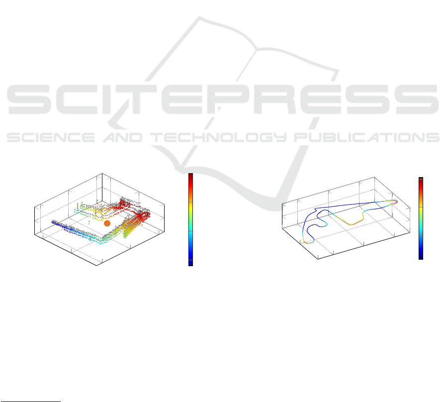
Figure 4 exemplarily illustrates a resulting continuous

PCM. The whole pipeline is implemented as a stan-

100

−500

−450

−400

x [m]

y [m]

z [m]

Translation [m]

Figure 4: Excerpt of a ﬁnal PCM with color-coded point

deformations by the Rubber-Sheet Transformation at the

YMC. Gray points represent the PCM after Rigid Alignment

with the orange mark being a selected CP subdividing the

excerpt into tetrahedra.

dalone ROS 2

package, leveraging RVIZ to provide

an interactive visualization of the ﬁnal result.

https://ros.org/

4 RESULTS

Both datasets, the YMC, and the KITTI dataset,

comprise RTK-corrected GNSS positions and LiDAR

point clouds, used as input to FlexCloud. As georefer-

encing requires the GNSS positions in a global frame,

raw data of the KITTI dataset is used. However, it

is noted at this point that due to the urban environ-

ment in sequence 00 of the KITTI dataset, the GNSS

positions feature high standard deviations for several

sections. The GNSS positions recorded at the YMC

are post-processed and show standard deviation in the

centimeter range, except for short occlusions. The

initial odometry trajectory and corresponding PCM

are created as described in Section 3. The evaluation

consists of two parts: First, we present quantitative

results on the deviation of the ﬁnal odometry to the

GNSS trajectory. For this, the Euclidean norm is com-

puted for each point on the odometry trajectory and its

corresponding point on the GNSS trajectory after the

Keyframe Interpolation. In contrast to the Rubber-

Sheet transformation, which only uses selected CPs,

the evaluation is conducted on all trajectory points

without excluding points with high standard devia-

tion. The second part of the evaluation is conducted

on publicly available satellite imagery. This enables a

qualitative evaluation with an external data source.

The resulting trajectories after the Keyframe Interpo-

lation consist of 2560 and 1550 poses for the YMC

and the KITTI dataset, respectively. To improve the

understanding of the pipeline, intermediate results are

presented for the YMC. Figure 5 shows the devia-

−500

500

−500

500

−200

200

x [m]

y [m]

z [m]

Deviation from GNSS [m]

Figure 5: Deviation of the odometry to the GNSS trajectory

(gray) after Rigid Alignment at the YMC.

tion of the odometry to the GNSS trajectory after the

Rigid Alignment step. Although the two trajectories

are optimally aligned with a rigid transformation at

this point, the deviation exceeds 15 m in certain sec-

tions. However, as the deviation is not constant, this

highlights the distortion of the trajectory and thus the

need for the Rubber-Sheet Transformation.

FlexCloud: Direct, Modular Georeferencing and Drift-Correction of Point Cloud Maps

161

Figure 6 illustrates the triangulation of the odom-

etry trajectory in the Rubber-Sheet Transformation.

First, the CPs are selected based on the conﬁguration,

and the maximum allowed standard deviation of the

GNSS positions (Figure 6a). In the second step, the

corner points of the enclosing cuboid are added, and

the Delaunay triangulation is computed.

Leveraging the transformation matrices computed

from the triangulation, the Rubber-Sheet Transforma-

tion is applied according to Equation 5 to the odom-

etry trajectory and the PCM. The deviation of the ﬁ-

nal odometry to the GNSS trajectory using 200 CPs

for the YMC is illustrated in Figure 7. Comparing

the ﬁnal deviation to the intermediate results after

the Rigid Alignment step (Figure 5), the beneﬁt of

the Rubber-Sheet Transformation in rectifying the tra-

jectory is clearly visible. Except for a short section

(x ≈ 400 m,y ≈ −800 m), where no CPs are selected

following high GNSS standard deviations, the devia-

tion falls below 1 m for the entire trajectory. The re-

sults for sequence 00 of the KITTI dataset in Figure 8

show similar results. Analogous to the YMC, the de-

viation increases within a section in the middle of the

trajectory due to high GNSS standard deviations pre-

venting the CP selection. As this shows the inﬂuence

of the amount and location of the CPs, Table 1 com-

pares the results of different quantities of CPs statis-

tically. For both datasets, the MAE decreases with an

Table 1: Quantitative results for the mean absolute error

(MAE), the standard deviation (STDDEV), and the maxi-

mum value (MAX) of the deviation of the georeferenced

odometry trajectory to the GNSS trajectory. Results are

provided for different amounts of CP n

with a standard

deviation threshold of 0.05 m and 0.25 m for the YMC and

the KITTI dataset, respectively.

Dataset | n

Metric in m

MAE STDDEV MAX

Yas Marina

Circuit

10 1.71 1.59 9.11

50 0.25 0.32 2.56

100 0.13 0.16 1.43

200 0.08 0.11 1.27

KITTI 00

10 1.26 0.77 4.03

50 0.60 0.77 3.71

150 0.47 0.83 4.07

increasing amount of CPs, leading to an average er-

ror of 0.08 m and 0.47 m for the YMC and the KITTI

dataset, respectively. This is expected as the distance

between successive CPs decreases. The larger value

for the KITTI dataset follows from an overall worse

quality of the GNSS positions. While STDDEV and

MAX also decrease with an increasing amount of CPs

for the YMC, this is not observable for the KITTI

dataset. This is due to the long section with insufﬁ-

cient GNSS accuracy in the middle of the trajectory.

It is noticeable that for n

= 10, the KITTI results are

superior to the YMC despite the worse quality of the

GNSS trajectory. This can be explained by the shorter

overall length of the KITTI dataset, causing a reduced

distance between consecutive CPs.

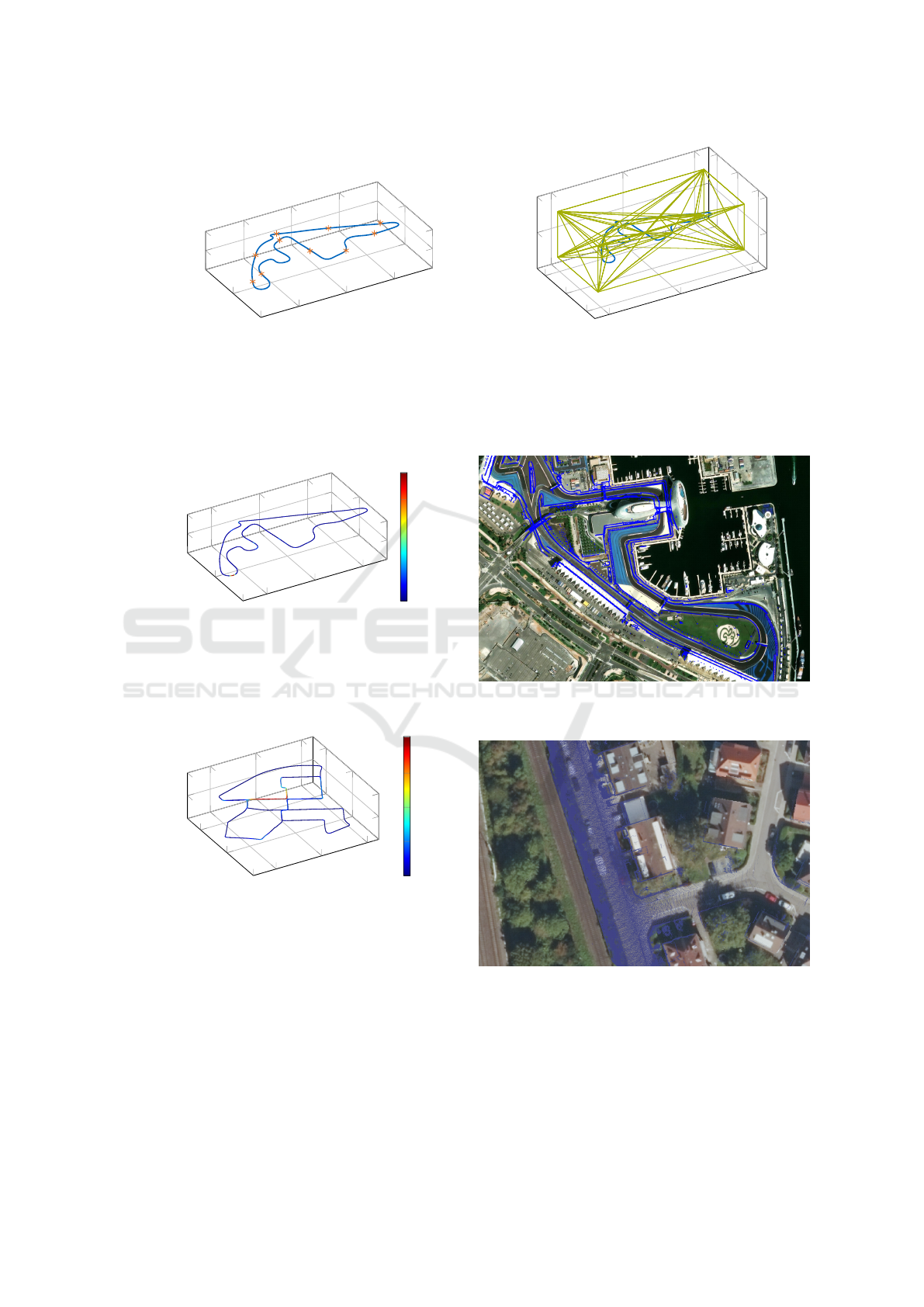
We leverage aerial photography to evaluate the results

independently of the GNSS positions, which are also

used as input to FlexCloud. Although this does not

enable a quantitative but a qualitative evaluation, it al-

lows further investigation of the performance of Flex-

Cloud, especially within the sections with high GNSS

uncertainty. For the YMC, the south part is visualized

over satellite imagery from ESRI (Esri, 2024) (Fig-

ure 9). A visual comparison indicates a strong over-

lap between the PCM and the satellite image, espe-

cially in the turn in the southeast of the image. Al-

though Figure 7 shows an increased deviation be-

tween the trajectories in this section, no deterioration

in the overlap is visible. This proves the ability of

FlexCloud to enable reliable georeferencing even for

short sections with insufﬁcient GNSS coverage.

As the KITTI dataset was recorded in the state of

Baden-W

urttemberg, Germany, public orthophotos

with a resolution of 20 cm are available for evalua-

tion (Figure 10). The shown excerpt is taken from

the southwest of the trajectory (x ≈ −60m,y ≈ 70m)

featuring good GNSS coverage. From the high res-

olution of the orthophoto, it is visible that the road

boundaries and building structures of the PCM ac-

curately match the orthophoto. This indicates that

PCMs georeferenced with FlexCloud can reach the

required accuracy for HD maps given a global trajec-

tory with sufﬁcient accuracy.

5 DISCUSSION

The presented results demonstrate that FlexCloud can

accurately georeference a given local PCM based on

the corresponding odometry and GNSS trajectory.

Nevertheless, our approach still features limitations

and areas for improvement, which are discussed in

this section. By introducing the Keyframe Interpo-

lation, we can directly utilize the GNSS trajectory

recorded by the MMS to generate CPs for georefer-

encing. Although this avoids the need for additional

measurements, it has the following limitations: To

reach an accuracy sufﬁcient for autonomous driving

applications, the MMS needs to be equipped with

an expensive RTK-corrected GNSS receiver. Fur-

thermore, the Keyframe Interpolation requires proper

https://www.lgl-bw.de/

VEHITS 2025 - 11th International Conference on Vehicle Technology and Intelligent Transport Systems

162

−500

500

−500

500

−200

200

x [m]

y [m]

z [m]

(a) Automatically selected CP (orange dots) on odometry tra-

jectory.

−500

500

−1,000

1,000

−500

500

x [m]

y [m]

z [m]

(b) Tetrahedra of resulting Delaunay triangulation.

Figure 6: Exemplary triangulation of the odometry trajectory (blue) using n

= 10 CP on the YMC. The size of the enclosing

cuboid equals 0.1 and 10 times the expansion of the trajectory in x/y and z, respectively.

−500

500

−500

500

−200

200

x [m]

y [m]

z [m]

Deviation from GNSS [m]

Figure 7: Final deviation of the odometry trajectory after

Rubber-Sheet Transformation using n

= 200 CP at the

YMC.

200

400

200

400

−100

100

x [m]

y [m]

z [m]

Deviation from GNSS [m]

Figure 8: Final deviation of the odometry trajectory after

Rubber-Sheet Transformation using n

= 150 CP on se-

quence 00 of the KITTI dataset (Geiger et al., 2012).

time synchronization between the GNSS receiver and

the LiDAR, as the interpolation leverages the times-

tamp differences between the trajectory positions.

The Rubber-Sheet Transformation leverages several

CPs, a subset of all positions of the trajectories, to

compute the transformation of the PCM. By exclud-

ing GNSS positions with high uncertainty from being

Figure 9: Visualization of PCM of the YMC on satellite

imagery from ESRI (Esri, 2024).

Figure 10: Visualization of PCM of KITTI sequence 00

over orthophotos of the State Ofﬁce for Geoinformation and

Rural Development (LGL)

of Baden-W

urttemberg.

selected as CP, these sections can still be georefer-

enced to a certain extent. However, this requires a

reliable standard deviation estimation of the GNSS

receiver. Furthermore, our current implementation

FlexCloud: Direct, Modular Georeferencing and Drift-Correction of Point Cloud Maps

163

does not utilize the actual values of the GNSS stan-

dard deviation but only excludes high values based

on a ﬁxed threshold. Hence, additional focus must

be spent on post-processing the GNSS positions, e.g.,

using curvature correction. Another point to be in-

vestigated is the shape structure surrounding the tra-

jectories/map during the Rubber-Sheet Transforma-

tion. Although the rectangular cuboid used within this

work shows robust results, limitations arise, e.g., for

trajectories/maps, where the surrounding cuboid fea-

tures large variations in the side lengths. An alterna-

tive approach would be the replacement of the cuboid

with a polygon-like shape.

6 CONCLUSION

FlexCloud provides a framework for direct georef-

erencing and drift-correction of local PCMs cre-

ated from SLAM. Following the modular design,

our approach can be combined with different SLAM

pipelines, utilizing only the generated odometry

trajectory and local PCM. By implementing the

Keyframe Interpolation, the pipeline can directly

leverage the GNSS positions recorded with an MMS,

avoiding the need for additional measurements. The

Rubber-Sheet Transformation enables rectiﬁcation of

the local PCM and georeferencing of short sections

without accurate GNSS positions. Although our ap-

proach still features limitations, it provides the op-

portunity to georeference PCMs with high accuracy,

allowing their usage for map-based localization al-

gorithms. Future work on the pipeline needs to fo-

cus on the boundary shape used for the Rubber-Sheet

Transformation and improved processing of the initial

GNSS positions based on their standard deviation.

ACKNOWLEDGEMENTS

As the ﬁrst author, Maximilian Leitenstern initiated

and designed the paper’s structure. He contributed

to designing and implementing the overall pipeline

concept. Christian Bolea-Schaser and Marko Al-

ten contributed to designing and implementing the

Rubber-Sheet Transformation and the Keyframe In-

terpolation during their student research project, re-

spectively. Dominik Kulmer, Marcel Weinmann, and

Markus Lienkamp revised the paper critically for im-

portant intellectual content. Markus Lienkamp gives

ﬁnal approval for the version to be published and

agrees to all aspects of the work. As a guarantor, he

accepts responsibility for the overall integrity of the

paper.

REFERENCES

Bao, Z., Hossain, S., Lang, H., and Lin, X. (2022). High-

Deﬁnition Map Generation Technologies For Au-

tonomous Driving. ArXiv, abs/2206.05400.

Bao, Z., Hossain, S., Lang, H., and Lin, X. (2023). A re-

view of high-deﬁnition map creation methods for au-

tonomous driving. Engineering Applications of Artiﬁ-

cial Intelligence, 122:106125.

Chen, X., Milioto, A., Palazzolo, E., Giguere, P., Behley, J.,

and Stachniss, C. (2019). SuMa++: Efﬁcient LiDAR-

based Semantic SLAM. In 2019 IEEE/RSJ Interna-

tional Conference on Intelligent Robots and Systems

(IROS). IEEE.

Esri (2024). Arcgis world imagery. Available at:

https://www.arcgis.com/apps/mapviewer/index.

html?layers=10df2279f9684e4a9f6a7f08febac2a9

(accessed on 2024-11-29).

Geiger, A., Lenz, P., Stiller, C., and Urtasun,

R. (2013). Vision meets robotics: The

KITTI dataset. The International Journal of

Robotics Research, 32(11):1231–1237. eprint:

https://doi.org/10.1177/0278364913491297.

Geiger, A., Lenz, P., and Urtasun, R. (2012). Are we ready

for autonomous driving? The KITTI vision bench-

mark suite. In 2012 IEEE Conference on Computer

Vision and Pattern Recognition, pages 3354–3361.

Gillman, D. (1985). Triangulations for rubber-sheeting.

In Proceedings of 7th International symposium on

computer assisted cartography (AutoCarto 7), volume

199.

Groves, P. (2013). Principles of GNSS, Inertial, and Mul-

tisensor Integrated Navigation Systems, Second Edi-

tion. Artech.

Hariz, F., Souiﬁ, H., Leblanc, R., Bouslimani, Y., Ghribi,

M., Langin, E., and Mccarthy, D. (2021). Direct Geo-

referencing 3D Points Cloud Map Based on SLAM

and Robot Operating System. In 2021 IEEE Inter-

national Symposium on Robotic and Sensors Environ-

ments (ROSE), pages 1–6.

Hess, W., Kohler, D., Rapp, H., and Andor, D. (2016). Real-

time loop closure in 2d lidar slam. In 2016 IEEE In-

ternational Conference on Robotics and Automation

(ICRA), pages 1271–1278.

Jamin, C., Pion, S., and Teillaud, M. (2024). 3D triangula-

tions. In CGAL User and Reference Manual. CGAL

Editorial Board, 6.0.1 edition.

Jeong, J., Yoon, J. Y., Lee, H., Darweesh, H., and Sung,

W. (2022). Tutorial on High-Deﬁnition Map Gener-

ation for Automated Driving in Urban Environments.

Sensors, 22(18).

Khoche, A., Wozniak, M. K., Duberg, D., and Jensfelt, P.

(2022). Semantic 3D Grid Maps for Autonomous

Driving. 2022 IEEE 25th International Conference

on Intelligent Transportation Systems (ITSC), pages

2681–2688.

Koide, K., Miura, J., and Menegatti, E. (2019). A

portable three-dimensional LIDAR-based system for

long-term and wide-area people behavior mea-

surement. International Journal of Advanced

VEHITS 2025 - 11th International Conference on Vehicle Technology and Intelligent Transport Systems

164

Robotic Systems, 16(2):1729881419841532. eprint:

https://doi.org/10.1177/1729881419841532.

Koide, K., Miura, J., Yokozuka, M., Oishi, S., and Banno,

A. (2021). Interactive 3D Graph SLAM for Map

Correction. IEEE Robotics and Automation Letters,

6(1):40–47.

Lasse Klingbeil (2023). Georeferencing of Mobile Mapping

Data. PhD Thesis, Rheinische Friedrich-Wilhelms-

Universit

at Bonn.

Leitenstern, M., Sauerbeck, F., Kulmer, D., and Betz, J.

(2024). FlexMap Fusion: Georeferencing and Auto-

mated Conﬂation of HD Maps with OpenStreetMap.

In 35th IEEE Intelligent Vehicles Symposium, IV

2024, IEEE Intelligent Vehicles Symposium, Proceed-

ings, pages 272–278. Institute of Electrical and Elec-

tronics Engineers Inc.

Liu, W., Li, Z., Sun, S., Du, H., and Sotelo, M. A. (2021).

Georeferencing kinematic modeling and error correc-

tion of terrestrial laser scanner for 3D scene recon-

struction. Automation in Construction, 126:103673.

Marvin S. White, J. and Grifﬁn, P. (1985). Piecewise lin-

ear rubber-sheet map transformation. The American

Cartographer, 12(2):123–131.

Oria-Aguilera, H., Alvarez-Perez, H., and Garcia-Garcia,

D. (2018). Mobile LiDAR Scanner for the Gener-

ation of 3D Georeferenced Point Clouds. In 2018

IEEE International Conference on Automation/XXIII

Congress of the Chilean Association of Automatic

Control (ICA-ACCA), pages 1–6.

Osada, E., So

snica, K., Borkowski, A., Owczarek-

Wesołowska, M., and Gromczak, A. (2017). A Direct

Georeferencing Method for Terrestrial Laser Scanning

Using GNSS Data and the Vertical Deﬂection from

Global Earth Gravity Models. Sensors, 17(7).

Paffenholz, J.-A. (2012). Direct geo-referencing of 3D

point clouds with 3D positioning sensors. PhD Thesis,

Leibniz-Universit

at Hannover.

Sauerbeck, F., Kulmer, D., Pielmeier, M., Leitenstern, M.,

Weiß, C., and Betz, J. (2023). Multi-lidar localization

and mapping pipeline for urban autonomous driving.

In 2023 IEEE SENSORS, pages 1–4.

Schuhmacher, S. and Boehm, J. (2005). Georeferencing

of Terrestrial Laserscanner Data for Applications in

Architectural Modelling. International Archives of

Photogrammetry, Remote Sensing and Spatial Infor-

mation Sciences, 36.

Seif, H. G. and Hu, X. (2016). Autonomous Driving in the

iCity—HD Maps as a Key Challenge of the Automo-

tive Industry. Engineering, 2(2):159–162.

Shan, T. and Englot, B. (2018). LeGO-LOAM: Lightweight

and Ground-Optimized Lidar Odometry and Mapping

on Variable Terrain. In 2018 IEEE/RSJ International

Conference on Intelligent Robots and Systems (IROS),

pages 4758–4765.

Shan, T., Englot, B., Meyers, D., Wang, W., Ratti, C., and

Rus, D. (2020). LIO-SAM: Tightly-coupled Lidar In-

ertial Odometry via Smoothing and Mapping.

eprint:

2007.00258.

Srinara, S., Chiu, Y.-T., Chen, J.-A., Chiang, K.-W., Tsai,

M.-L., and El-Sheimy, N. (2023). Strategy on High-

Deﬁnition Point Cloud Map Creation for Autonomous

Driving in Highway Environments. The Interna-

tional Archives of the Photogrammetry, Remote Sens-

ing and Spatial Information Sciences, XLVIII-1/W2-

2023:849–854.

Umeyama, S. (1991). Least-squares estimation of transfor-

mation parameters between two point patterns. IEEE

Transactions on Pattern Analysis and Machine Intel-

ligence, 13(4):376–380.

Vizzo, I., Guadagnino, T., Mersch, B., Wiesmann, L.,

Behley, J., and Stachniss, C. (2023). KISS-ICP: In

Defense of Point-to-Point ICP Simple, Accurate, and

Robust Registration If Done the Right Way. IEEE

Robotics and Automation Letters, 8(2):1029–1036.

Publisher: Institute of Electrical and Electronics En-

gineers (IEEE).

Wilkinson, B., Mohamed, A., and Dewitt, B. (2015).

Dual-Antenna Terrestrial Laser Scanner Georeferenc-

ing Using Auxiliary Photogrammetric Observations.

Remote Sensing, 7(9):11621–11638.

Wilkinson, B. E., Mohamed, A. H., Dewitt, B. A., and

Seedahmed, G. H. (2010). A Novel Approach to Ter-

restrial Lidar Georeferencing. Photogrammetric En-

gineering & Remote Sensing, 76(6):683–690.

Xu, W., Cai, Y., He, D., Lin, J., and Zhang, F. (2021).

FAST-LIO2: Fast Direct LiDAR-inertial Odometry.

eprint: 2107.06829.

Xu, W. and Zhang, F. (2021). FAST-LIO: A Fast, Ro-

bust LiDAR-inertial Odometry Package by Tightly-

Coupled Iterated Kalman Filter. eprint: 2010.08196.

Zhang, J. and Singh, S. (2014). LOAM : Lidar Odometry

and Mapping in real-time. Robotics: Science and Sys-

tems Conference (RSS), pages 109–111.

FlexCloud: Direct, Modular Georeferencing and Drift-Correction of Point Cloud Maps

165