Prompt-Driven Time Series Forecasting with Large Language Models

Zairo Bastos

, João David Freitas

, José Wellington Franco

and Carlos Caminha

1,2

Universidade Federal do Ceará - UFC, Brazil

Programa de Pós Graduação em Informática Aplicada - PPGIA/UNIFOR, Brazil

Keywords:

Large Language Models, Time Series, Transformers, Univariate.

Abstract:

Time series forecasting with machine learning is critical across various ﬁelds, with Ensemble models and Neu-

ral Networks commonly used to predict future values. LSTM and Transformers architecture excel in modeling

complex patterns, while Random Forest has shown strong performance in univariate time series forecasting.

With the advent of Large Language Models (LLMs), new opportunities arise for their application in time series

prediction. This study compares the forecasting performance of Gemini 1.5 PRO against Random Forest and

LSTM using 40 time series from the Retail and Mobility domains, totaling 65,940 time units, evaluated with

SMAPE. Results indicate that Gemini 1.5 PRO outperforms LSTM by approximately 4% in Retail and 6.5%

in Mobility, though it underperforms Random Forest by 5.5% in Retail and 1% in Mobility. In addition to

this comparative analysis, the article contributes a novel prompt template designed speciﬁcally for time series

forecasting, providing a practical tool for future research and applications.

1 INTRODUCTION

Time series forecasting is a fundamental task in var-

ious ﬁelds, including economics, ﬁnance, logistics,

and healthcare. Machine learning models, such as en-

sembles and neural networks, have been widely em-

ployed to capture temporal patterns and predict fu-

ture values based on historical data (Lim and Zohren,

2021). Neural network architectures, such as LSTM

(Long Short-Term Memory) and Transformers, are

known for their ability to model complex and non-

linear patterns in time series, while ensemble-based

machine learning methods, such as Random Forest,

have shown robust performance, especially in univari-

ate forecasting problems (Kane et al., 2014) (Freitas

et al., 2023).

With the advent of Large Language Models

(LLMs), new possibilities have emerged for time se-

ries forecasting. These models, originally designed

for natural language processing tasks, have demon-

strated versatility in a variety of applications, includ-

ing computer vision (Wang et al., 2024), information

extraction (Goel et al., 2023) (Almeida and Caminha,

2024), code generation (Gu, 2023), dataset generation

(Silva et al., 2024) (Karl et al., 2024) and time series

analysis (Jin et al., 2023a). The ability of these mod-

els to capture complex patterns in large volumes of

data suggests untapped potential for their application

in time series forecasting.

This paper investigates the effectiveness of a state-

of-the-art LLM, speciﬁcally Gemini 1.5 PRO, in uni-

variate time series forecasting, comparing its perfor-

mance with two traditional models: Random Forest

and LSTM. The comparison is made using 40 time

series from two distinct domains: Retail and Mobil-

ity, covering a total of 65,940 time units. A large ex-

periment with 1,200 predictions was conducted, ana-

lyzing 13,680 time units across both domains. The

metric chosen for evaluation is SMAPE (Symmet-

ric Mean Absolute Percentage Error), widely used to

measure accuracy in time series forecasting.

The results of this research reveal that Gemini

1.5 PRO outperforms LSTM by approximately 4%

in the Retail domain and 6.5% in the Mobility do-

main. However, the LLM model underperforms Ran-

dom Forest, with a difference of 5.5% in Retail and

1% in Mobility. In addition to the comparative eval-

uation, this study contributes to developing a prompt

template that facilitates time series forecasting, offer-

ing a practical tool for future research and applica-

tions.

This article is organized as follows: Section 2

presents the related works, reviewing key works and

recent advances in applying LLMs to time series fore-

casting. Section 3 details the methodology used, in-

cluding the description of the datasets, the forecasting

Bastos, Z., Freitas, J. D., Franco, J. W. and Caminha, C.

Prompt-Driven Time Series Forecasting with Large Language Models.

DOI: 10.5220/0013363800003929

Paper published under CC license (CC BY-NC-ND 4.0)

In Proceedings of the 27th International Conference on Enterprise Information Systems (ICEIS 2025) - Volume 1, pages 309-316

ISBN: 978-989-758-749-8; ISSN: 2184-4992

309

models employed, and the prompt speciﬁcally devel-

oped for LLMs. Section 4 discusses the results of the

experiments, comparing the performance of Gemini

1.5 PRO with traditional models. Section 4 also offers

a critical analysis of the results, highlighting the main

contributions of this study and the observed limita-

tions. Finally, Section 5 concludes the paper, suggest-

ing future directions for research that seek to explore

and expand the use of LLMs in time series forecast-

ing.

2 RELATED WORK

LLMs beneﬁt various applications, such as in com-

puter vision and natural language processing (Jin

et al., 2023a). In (Jin et al., 2023b), it is shown that al-

though time series forecasting has not yet reached the

same advances as these more prominent areas, time

series forecasting can beneﬁt from LLMs in certain

applications and modeling approaches. In this con-

text, we will highlight some of the key works in the

state of the art.

In (Jin et al., 2023b), a reprogramming framework

is proposed to adapt LLMs for time series forecasting

while keeping the model intact. The central idea is

to reprogram the input time series into text represen-

tations, including declarative sections, that are more

naturally suited to the capabilities of language mod-

els. One of the main advantages pointed out by the

authors is that the framework naturally aligns with the

language models’ strengths.

The work by (Liu et al., 2024a) presents a frame-

work that aligns multivariate time series data with

pre-trained LLMs by generating a single data input

for a Transformer model (Vaswani et al., 2017), which

performs the time series prediction. As presented

in (Zeng et al., 2023), Transformer models, with

their powerful self-attention mechanism, can cause

the loss of temporal information. When working di-

rectly with time series data, this can lead to disorder

in the data, which may result in performance issues.

Thus, the framework proposed by (Liu et al., 2024a)

aims to solve this problem, improving the model’s

performance compared to other strategies and reduc-

ing model inference time.

(Liu et al., 2024b) proposes the Spatial-Temporal

Large Language Model (ST-LLM) for trafﬁc forecast-

ing. Trafﬁc forecasting is a time series task that aims

to predict future trafﬁc characteristics based on his-

torical data, a crucial component of intelligent trans-

portation systems. The main idea of the approach

is to use the timesteps as an input token in a spatio-

temporal network layer, focusing on spatial locations

and temporal patterns. The model was evaluated on

real-world trafﬁc data and showed prominent results.

This article differs from others by exploring, in an

unprecedented way, the application of a Large Lan-

guage Model (LLM) in the task of univariate time se-

ries forecasting. While previous works have focused

on frameworks that reprogram LLMs to adapt to tem-

poral forecasting or on approaches that integrate tradi-

tional models with LLMs, our research adopts a direct

approach, using an LLM for time series forecasting

without the need for structural modiﬁcations or com-

binations with other models. Furthermore, we have

developed a speciﬁc prompt to guide the LLM in the

forecasting process, contributing a tool that can be

reused in different scenarios and with future LLMs.

This approach allows for a comparative analysis be-

tween the LLM and traditional methods such as Ran-

dom Forest and LSTM, providing new insights into

the potential and limitations of LLMs in this area.

3 METHOLOGY

3.1 Dataset

The ﬁrst dataset comprises time series of product

sales from a retail store, speciﬁcally in the supermar-

ket sector, located in Fortaleza-CE. Information was

obtained on sales of twenty products from the A curve

(items with the greatest contribution to the store’s rev-

enue) over the period from January 2, 2017, to April

30, 2019, totaling approximately 850 days. The sales

of the products, by units or kilograms, were aggre-

gated by day for each of the products analyzed, and

the ﬁnal time series were constructed. The product

identiﬁers were anonymized. In this article, we used

the data from January 2, 2017, to January 2, 2019,

as the training set, while the test data covered the pe-

riod from January 3, 2019, to March 3, 2019. Figure

1(B) illustrates a daily sales time series for one of the

A-curve products over a sample of 200 days.

The second dataset consists of time series of the

number of passengers boarding the twenty most used

bus lines in Fortaleza’s public transportation system

(Ceará). Passengers in the bus system use a smart

card with a user identiﬁer, and each time this card is

used, a boarding record is made. The data was pro-

vided by the Fortaleza City Hall and has been used

in other articles, in compliance with the General Data

Protection Law (LGPD) (Caminha and Furtado, 2017;

Ponte et al., 2018; Bomﬁm et al., 2020; Ponte et al.,

2021). In this article, the training data covers the pe-

riod from March 1, 2018, to June 4, 2018, while the

test data spans a week (168 hours), from June 5, 2018,

ICEIS 2025 - 27th International Conference on Enterprise Information Systems

310

Time in hours

Time in days

Sales

Bus Boarding

Figure 1: Examples of time series. (A) Number of passengers on a bus route during the ﬁrst 200 hours. (B) Sales data of a

product over 200 days.

to June 11, 2018. This generated twenty time series,

each with more than 2,280 hours of boardings in the

training set and 168 hours in the test set. Figure 1(A)

illustrates a time series of hourly boardings for a bus

line, detailing the seasonal patterns that occur in the

vehicles over a sample of around 9 days (200 hours).

The retail domain data exhibits more complex and

varied seasonal patterns compared to the mobility do-

main data. Retail sales undergo signiﬁcant variations

due to factors such as promotions, seasonal events,

and supply-demand ﬂuctuations, which are not fully

captured in the dataset used in this study. This re-

sults in distinct seasonal patterns in each time series,

where certain products may experience unpredictable

sales spikes, depending on promotional campaigns or

market changes. On the other hand, the mobility data,

which records the number of passengers boarding bus

lines, shows more regular seasonal patterns, with pre-

dictable variations based on factors such as weekdays

and times of the day. Although some lines are bus-

ier on weekends or have higher demand on speciﬁc

weekdays, the variation within each series is rela-

tively low, making the temporal patterns more homo-

geneous and less complex to model.

3.2 Modeling and Model Training

The sliding windows technique was used in the mod-

eling process for the time series forecasting problem

(Chu, 1995) for the Random Forest and LSTM mod-

els. The sliding windows technique involves dividing

the time series into smaller, ﬁxed-size segments (w).

The term "sliding" refers to the process of shifting the

window to the right along the series by a certain step

size (p), allowing for the construction of a training

dataset.

Sliding windows serve as a mechanism to trans-

form the time series into a labeled dataset, where each

window contains a set of observations from the past

of the time series, which are considered as the input

for the forecasting models. The observation imme-

diately after the end of the window is deﬁned as the

target value to be predicted, given the previous win-

dow. This technique is particularly suited for super-

vised regression-based machine learning methods for

time series forecasting.

Figure 2 illustrates the process of generating input

and output examples used to train AI models. A daily

time series, shown in green as an example, is trans-

formed into a supervised dataset. A window of size

w is applied, generating the ﬁrst input sample with w

values, representing the features that the models must

learn. In addition to the information from the window,

a time embedding is concatenated, providing tempo-

ral information about the target variable, such as the

time of day (speciﬁcally for mobility series), the day

of the week, the day of the month, and the day of the

year. These features allow the models to learn tempo-

ral dependencies from past observations, helping to

predict future values. The day immediately after the

window represents the target variable to be predicted.

The window is then shifted p steps to the right to gen-

erate new samples for the dataset, repeating the pro-

cess across the entire series. Depending on w and p,

there may be data overlap, reinforcing the discovery

of patterns and increasing the number of training sam-

ples. The ﬁnal part of the ﬂow in Figure 2 illustrates

the training process of machine learning models from

the labeled data generated in the previous steps.

For the retail time series, a window size of w =90

(approximately three months) was used, while for the

urban mobility time series, the window size was de-

ﬁned as w = 168 (exactly one week). These values

were chosen because they cover a sufﬁcient period to

Prompt-Driven Time Series Forecasting with Large Language Models

311

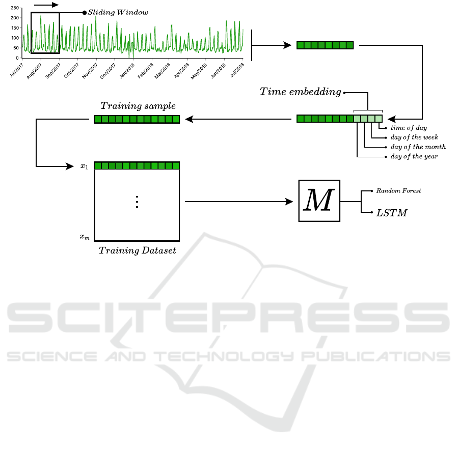
Figure 2: Construction of examples using the concept of sliding windows.

capture the main seasonal patterns in the series, ensur-

ing that the most signiﬁcant variations are reﬂected in

the modeled examples.

The models used were an ensemble model (Ran-

dom Forest) and a neural network (LSTM). In Ran-

dom Forest (Breiman, 2001), default parameters from

Scikit-learn (Pedregosa et al., 2011) were used. For

the LSTM (Hochreiter and Schmidhuber, 1997), the

Tensorﬂow implementation (Abadi et al., 2016) was

used, with the following parameters: neurons = 200,

batch_size = 32, ReLU activation function, epochs =

200, 20% validation, and the Adam optimizer with a

learning rate of 0.0001.

The choice of Random Forest and LSTM models

for time series forecasting in this research is justiﬁed

by the nature of the analyzed time series, which are

univariate and do not have a large time span. Ran-

dom Forest is known for its robustness in univariate

problems, especially when dealing with short time

series with relatively simple seasonal patterns (Fre-

itas et al., 2023). LSTM is widely used to capture

short- and medium-term temporal dependencies and

patterns, being effective in time series with moder-

ately complex structures (Sagheer and Kotb, 2019).

The use of Transformers, although powerful, would

not be indicated in this context because these models

are more appropriate for time series involving large

amounts of time data or multiple characteristics that

vary simultaneously (multivariate series) with com-

plex seasonal patterns (Zeng et al., 2023). Since the

time series used in this research do not have these

characteristics, applying Transformers would be un-

necessary and potentially less efﬁcient, thus justify-

ing the choice of simpler models better suited to the

available data.

3.3 Developed Prompt

In this study, the modeling process for time series

forecasting using LLMs differs signiﬁcantly from the

approach used with models like LSTM and Random

Forest, where the sliding windows concept is essen-

tial. In the case of LLMs, it does not make sense

to use a window-based approach, as the model oper-

ates on the entire sequence of data provided at once,

without the need to fragment the data into temporal

blocks. Instead, the modeling is guided by an elabo-

rate prompt that instructs the model to make predic-

tions based on the patterns and trends captured in the

data.

Figure 3 presents the prompt used in this study to

perform time series forecasts. This prompt was de-

signed to leverage the capabilities of an LLM, guid-

ing it to focus on the most relevant aspects of the time

series to generate the forecast. Below, we detail each

element of the prompt and explain its function:

• Variable h: Represents the number of days (or an-

other time unit, as deﬁned by the time_step vari-

able) to be predicted, that is, it deﬁnes the forecast

horizon that the model must consider when gener-

ICEIS 2025 - 27th International Conference on Enterprise Information Systems

312

ating future values;

• Variable time_step: Indicates the time unit of the

provided data, which can be hours, days, weeks,

months, etc. This variable helps the model under-

stand the data’s granularity and adjust its analy-

sis to accurately capture the relevant seasonal pat-

terns and trends for that periodicity;

• Variable training_data: Contains the time series

that will be used for forecasting. This time se-

ries is provided up to the limit that, in other mod-

els (LSTM and Random Forest), would be consid-

ered the end of the training set, excluding the test

data. This way, the LLM has access only to the

information that would be available in a real fore-

casting scenario, similar to the process performed

with other machine learning models;

• Variable context: Provides additional information

about the time period corresponding to certain po-

sitions in the value vector, such as the day of

the week. This temporal contextualization plays

a role similar to the modeling window used in

LSTM and Random Forest, helping the model

capture seasonal variations and speciﬁc patterns

when generating forecasts. Examples of the con-

tent of the context variable include:

For data with a time step in hours:

• Day 0: positions 432 to 455 (Monday);

• Day 1: positions 576 to 599 (Sunday);

• Day 2: positions 696 to 719 (Friday).

For data with a time step in days:

• position 0 - (Monday);

• position 1 - (Tuesday);

• position 2 - (Wednesday).

The designed prompt was structured to ensure that

the LLM focuses on predicting the sequence of future

values without generating code, explanations, or any

additional content that could interfere with the accu-

racy and efﬁciency of the forecasting process. The

model is instructed to provide exclusively a vector

containing the predicted values, starting immediately

after the last data provided.

This speciﬁc prompt design aims to exploit

LLMs’ ability to capture complex patterns, such as

trends and seasonality, holistically, without the need

to segment the time series into multiple windows.

This approach is especially useful for language mod-

els, which have strong generalization potential and

can identify global patterns in a single pass through

the data without relying on traditional time series

modeling techniques.

Context

You are a time series forecasting assistant tasked with

analyzing data from a speciﬁc time series.

The time series has data for {h} consecutive periods.

Each entry in the time series represents the incidence

of an event occurring every {time_step}.

Objective

Your goal is to forecast the incidence of an event for

the next {h} {time_step}, taking into account not only

the previous periods but also the overall context.

To do this accurately, consider:

• Seasonal Patterns: Recurring peaks and troughs

occurring at a certain periodicity.

• Trends: Rising or falling trends in the time series.

Output Rules:

After analyzing the provided data and understand-

ing the patterns, generate a forecast for the next {h}

{time_step}, with the following rules:

• The output should be a list containing only the

predicted values, without any additional explana-

tion or introductory text.

• Under no circumstances generate code;

• Under no circumstances generate an explanation

of what you did;

• Provide only and exclusively a vector containing

the requested number of numbers.

• The forecast should start immediately after the

last data provided.

Example Output for N={h}:

{data_prompt[:h]}

Additional Instructions:

• Weekly Patterns: Use the provided data to under-

stand seasonal patterns, such as incidence peaks at

certain times.

• Day of the Week: The day of the week also inﬂu-

ences the occurrence of events.

• Duration of an Event: The provided time se-

ries represents the occurrence of an event every

{time_step}.

Time series to be analyzed:

{training_data}

Context for the time period to be considered in the

forecast:

{context}

Generate a vector with {h} positions (N={h}) predict-

ing the sequence numbers:

Figure 3: Deﬁnition of the prompt used for time series

forecasts. The information appearing in braces represents

variables that are replaced whenever a new series forecast is

required.

Prompt-Driven Time Series Forecasting with Large Language Models

313

3.4 Execution Environment of the

Experiments

The Google API

was used to perform the infer-

ences with Gemini 1.5 PRO, always using a temper-

ature equal to one. To train and forecast with LSTM

and Random Forest, Python 3.11 was used, with Pan-

das 2.0.3 and Numpy 1.25.0 for data manipulation,

and Tensorﬂow 2.11.1 and Scikit-Learn 1.3.0, respec-

tively, for model creation.

3.5 Evaluation

The evaluation of the results was carried out us-

ing the Symmetric Mean Absolute Percentage Error

(SMAPE) (Makridakis, 1993), a metric chosen be-

cause it is percentage-based, which is particularly

relevant given that the retail dataset contains differ-

ent units (e.g., products sold by unit and by weight).

Furthermore, SMAPE is a geometric mean measure,

making it ideal for comparing the performance of

multiple models across a large number of forecasts,

as highlighted in (Kreinovich et al., 2014). SMAPE

is calculated as shown in Equation 1:

SMAPE =

∑

i=1

∣y

− ˆy

∣

∣y

∣+∣ ˆy

∣

×100 (1)

where ˆy

represents the predicted value, y

is the ob-

served actual value, and h is the total number of fore-

casted time units in the forecasting horizon.

For each of the 40 time series studied, ten fore-

casts were made for each evaluated model, with h =60

for the retail series and h =168 for mobility. For each

forecast, the respective SMAPE was calculated, and

the average SMAPE for each series was subsequently

obtained. In addition, the Standard Error of the Mean

(SEM) was calculated (Altman and Bland, 2005), as

shown in Equation 2:

SEM =

√

(2)

where n is the total number of forecasts made, which

in this study is always n =10.

4 RESULTS AND DISCUSSION

The forecasting results for the 40 time series from the

Retail and Mobility domains, using the models Gem-

ini 1.5 PRO, LSTM, and Random Forest, are pre-

sented in Table 1. The SMAPE (Symmetric Mean

https://cloud.google.com/vertex-ai/generative-

ai/docs/model-reference/gemini?hl=pt-br

Absolute Percentage Error) values and their respec-

tive standard errors (SEM) allow for the evaluation of

the forecasting accuracy for each individual time se-

ries.

In the Retail domain, the Random Forest model

demonstrated superiority in most of the time series,

with an average SMAPE of 36.22%, being the best

or tied (considering SEM) with the best model in 15

out of the 20 analyzed time series. The LSTM model,

on the other hand, presented an average SMAPE of

45.85%, while Gemini 1.5 PRO obtained a value of

41.80%.

Analyzing the individual time series, the Gemini

1.5 PRO model outperformed or tied with the other

models in seven time series (ids 3, 14, 15, 16, 18,

19, 20). The LSTM model, although it had a lower

performance in most of the time series, stood out in

three series (ids 3, 13, 19), where it tied with Gemini

1.5 PRO, and in two speciﬁc series (ids 3 and 19), it

slightly outperformed Random Forest.

In the Mobility domain, the model performances

were more balanced. Gemini 1.5 PRO achieved an

average SMAPE of 20.60%, LSTM reached 27.03%,

while Random Forest had an average SMAPE of

19.67%. Notably, Gemini 1.5 PRO outperformed or

tied with the other models in 11 out of 20 time series

(ids 4, 5, 9, 10, 12, 13, 15, 16, 17, 18, 19).

The results obtained in this study demonstrate that

the Large Language Model (LLM) Gemini 1.5 PRO

showed promising performance when compared to

traditional machine learning models, such as Random

Forest and LSTM, in the task of time series forecast-

ing. In several time series, especially in the Mobil-

ity domain, the LLM outperformed traditional algo-

rithms, which is particularly interesting considering

that the model used only its intrinsic language capa-

bilities to capture and infer seasonal patterns.

This result suggests that, although LLMs like

Gemini 1.5 PRO were not originally designed for time

series forecasting, their ability to model complex pat-

terns in varied data can be successfully explored un-

der certain conditions. The LLM’s capacity to gen-

eralize information and identify hidden patterns in

the data, which is crucial for natural language un-

derstanding, can also be useful in speciﬁc forecasting

scenarios, as evidenced by the results obtained with

the Mobility time series.

However, the worse results observed in the Retail

domain indicate that there are still signiﬁcant chal-

lenges to be overcome for the effective application of

LLMs in this area. The Retail time series, with their

more complex and diverse patterns, seem to demand

a level of specialization that LLMs cannot yet fully

achieve. The difﬁculty of the LLM in dealing with the

ICEIS 2025 - 27th International Conference on Enterprise Information Systems

314

Table 1: SMAPE values obtained in the experiments.

Retail Mobility

id Gemini LSTM RF id Gemini LSTM RF

1 55,59 ± 1,28 50,70 ± 0,02 33,69 ± 0,12 1 15,96 ± 0,73 12,23 ± 0,25 30,56 ± 2,84

2 50,53 ± 0,97 46,92 ± 0,07 39,48 ± 0,14 2 17,75 ± 0,14 25,39 ± 0,87 11,49 ± 0,04

3 46,41 ± 1,70 43,51 ± 1,20 45,94 ± 0,29 3 16,27 ± 0,55 14,34 ± 0,28 21,42 ± 0,59

4 18,80 ± 0,68 52,01 ± 0,52 13,97 ± 0,07 4 17,15 ± 2,16 36,89 ± 0,72 16,10 ± 0,56

5 85,45 ± 1,93 85,78 ± 0,06 70,13 ± 0,34 5 12,55 ± 1,47 21,65 ± 0,46 10,61 ± 0,50

6 43,83 ± 0,70 39,04 ± 0,07 22,56 ± 0,17 6 29,28 ± 0,13 28,17 ± 1,01 17,29 ± 2,40

7 45,64 ± 0,56 47,98 ± 0,73 35,88 ± 0,15 7 19,36 ± 0,35 20,68 ± 0,86 9,39 ± 0,05

8 30,77 ± 1,75 33,54 ± 0,79 24,84 ± 1,02 8 50,63 ± 0,70 18,78 ± 0,77 14,62 ± 0,54

9 37,21 ± 0,54 32,91 ± 0,04 30,41 ± 0,17 9 24,82 ± 1,05 26,50 ± 0,30 25,34 ± 0,52

10 45,12 ± 2,56 41,69 ± 0,16 32,52 ± 0,19 10 14,66 ± 0,55 31,03 ± 1,04 14,94 ± 0,06

11 36,83 ± 0,50 31,59 ± 0,02 30,56 ± 0,19 11 23,52 ± 0,86 32,24 ± 0,73 15,81 ± 0,07

12 21,89 ± 0,61 20,89 ± 0,47 18,91 ± 0,24 12 15,48 ± 0,35 24,90 ± 0,42 21,06 ± 0,40

13 36,55 ± 0,55 34,15 ± 0,06 35,01 ± 0,19 13 13,41 ± 0,82 40,97 ± 1,35 19,85 ± 1,07

14 22,95 ± 0,51 35,14 ± 0,82 26,92 ± 0,40 14 26,03 ± 0,76 23,02 ± 0,53 26,31 ± 2,24

15 33,22 ± 0,91 57,61 ± 2,00 33,23 ± 0,25 15 16,36 ± 0,25 30,19 ± 0,72 22,04 ± 0,39

16 27,55 ± 0,40 49,14 ± 0,46 29,79 ± 0,15 16 15,01 ± 0,55 25,45 ± 0,60 26,63 ± 0,53

17 31,90 ± 0,63 37,18 ± 0,09 25,92 ± 0,17 17 19,76 ± 0,36 26,61 ± 0,35 28,95 ± 2,86

18 61,79 ± 1,02 70,64 ± 0,84 62,21 ± 0,41 18 13,90 ± 0,95 39,67 ± 1,43 15,64 ± 0,70

19 29,08 ± 0,29 29,12 ± 0,65 37,59 ± 0,62 19 23,47 ± 0,69 25,94 ± 0,38 30,32 ± 0,29

20 74,85 ± 0,86 77,49 ± 0,44 74,91 ± 0,20 20 26,64 ± 1,13 35,92 ± 1,18 15,03 ± 0,14

µ 41,80 45,85 36,22 µ 20,60 27,03 19,67

variability and complexity of these time series points

to the need for model improvements or possibly the

integration of complementary techniques that can bet-

ter handle these data characteristics.

One of the contributions of this study is the de-

velopment of a speciﬁc prompt for time series fore-

casting, which can be reused in different LLMs as

new models are released. This allows researchers and

practitioners to evaluate the evolution of LLMs in the

task of time series forecasting over time, providing a

practical tool to track and explore the growing poten-

tial of these models in varied scenarios.

5 CONCLUSIONS

This study investigated the effectiveness of a Large

Language Model (LLM) in the task of time series

forecasting, comparing its performance with tradi-

tional machine learning models such as Random For-

est and LSTM. The results showed that, while the

LLM used, Gemini 1.5 PRO, demonstrated promis-

ing performance, especially in the time series from

the Mobility domain, its performance was inferior to

traditional methods in the Retail domain, where the

time series presented more complex and diverse pat-

terns.

One of the main contributions of this work is the

development of a speciﬁc prompt for time series fore-

casting, which can be reused in future studies with

different LLMs. This prompt allows for continuous

evaluation of LLMs’ evolution as new models are re-

leased, offering a solid foundation for future compar-

isons.

For future work, we propose evaluating open-

source LLMs in the task of time series forecasting.

The use of open-source models will provide greater

ﬂexibility in customization and experimentation, in

addition to allowing direct comparisons with propri-

etary models such as Gemini 1.5 PRO. This investi-

gation may reveal the potential of open-source LLMs

to capture complex temporal patterns and generalize

to different forecasting contexts.

Additionally, it is essential to expand the evalua-

tion to include larger and more complex time series,

which could provide a more comprehensive view of

the performance of LLMs. By including these series,

it will be possible to compare the results with state-

of-the-art models speciﬁcally designed to handle such

challenges, such as Transformers. This comparison

will be crucial to determine whether LLMs can effec-

tively compete with highly specialized models in sce-

narios where the complexity and variability of time

series are signiﬁcant.

REFERENCES

Abadi, M., Barham, P., Chen, J., Chen, Z., Davis, A., Dean,

J., Devin, M., Ghemawat, S., Irving, G., Isard, M.,

et al. (2016). Tensorﬂow: a system for large-scale ma-

chine learning. In Osdi, volume 16, pages 265–283,

USA. Savannah, GA, USA, USENIX Association.

Almeida, F. and Caminha, C. (2024). Evaluation of entry-

Prompt-Driven Time Series Forecasting with Large Language Models

315

level open-source large language models for informa-

tion extraction from digitized documents. In Anais

do XII Symposium on Knowledge Discovery, Mining

and Learning, pages 25–32, Porto Alegre, RS, Brasil.

SBC.

Altman, D. G. and Bland, J. M. (2005). Standard deviations

and standard errors. Bmj, 331(7521):903.

Bomﬁm, R., Pei, S., Shaman, J., Yamana, T., Makse, H. A.,

Andrade Jr, J. S., Lima Neto, A. S., and Furtado, V.

(2020). Predicting dengue outbreaks at neighbour-

hood level using human mobility in urban areas. Jour-

nal of the Royal Society Interface, 17(171):20200691.

Breiman, L. (2001). Random forests. Machine learning,

45:5–32.

Caminha, C. and Furtado, V. (2017). Impact of human mo-

bility on police allocation. In 2017 IEEE International

Conference on Intelligence and Security Informatics

(ISI), pages 125–127. IEEE.

Chu, C.-S. J. (1995). Time series segmentation: A slid-

ing window approach. Information Sciences, 85(1-

3):147–173.

Freitas, J. D., Ponte, C., Bomﬁm, R., and Caminha, C.

(2023). The impact of window size on univariate time

series forecasting using machine learning. In Anais do

XI Symposium on Knowledge Discovery, Mining and

Learning, pages 65–72. SBC.

Goel, A., Gueta, A., Gilon, O., Liu, C., Erell, S., Nguyen,

L. H., Hao, X., Jaber, B., Reddy, S., Kartha, R., et al.

(2023). Llms accelerate annotation for medical infor-

mation extraction. In Machine Learning for Health

(ML4H), pages 82–100. PMLR.

Gu, Q. (2023). Llm-based code generation method for

golang compiler testing. In Proceedings of the 31st

ACM Joint European Software Engineering Confer-

ence and Symposium on the Foundations of Software

Engineering, pages 2201–2203.

Hochreiter, S. and Schmidhuber, J. (1997). Long short-term

memory. Neural computation, 9(8):1735–1780.

Jin, M., Wang, S., Ma, L., Chu, Z., Zhang, J. Y., Shi,

X., Chen, P.-Y., Liang, Y., Li, Y.-F., Pan, S., et al.

(2023a). Time-llm: Time series forecasting by re-

programming large language models. arXiv preprint

arXiv:2310.01728.

Jin, M., Wen, Q., Liang, Y., Zhang, C., Xue, S., Wang,

X., Zhang, J., Wang, Y., Chen, H., Li, X., et al.

(2023b). Large models for time series and spatio-

temporal data: A survey and outlook. arXiv preprint

arXiv:2310.10196.

Kane, M. J., Price, N., Scotch, M., and Rabinowitz, P.

(2014). Comparison of arima and random forest time

series models for prediction of avian inﬂuenza h5n1

outbreaks. BMC bioinformatics, 15:1–9.

Karl, A., Fernandes, G., Pires, L., Serpa, Y., and Cam-

inha, C. (2024). Synthetic ai data pipeline for domain-

speciﬁc speech-to-text solutions. In Anais do XV Sim-

pósio Brasileiro de Tecnologia da Informação e da

Linguagem Humana, pages 37–47, Porto Alegre, RS,

Brasil. SBC.

Kreinovich, V., Nguyen, H. T., and Ouncharoen, R. (2014).

How to estimate forecasting quality: A system-

motivated derivation of symmetric mean absolute per-

centage error (smape) and other similar characteris-

tics. Departmental Technical Reports (CS).

Lim, B. and Zohren, S. (2021). Time-series forecasting with

deep learning: a survey. Philosophical Transactions of

the Royal Society A, 379(2194):20200209.

Liu, C., Xu, Q., Miao, H., Yang, S., Zhang, L., Long, C.,

Li, Z., and Zhao, R. (2024a). Timecma: Towards llm-

empowered time series forecasting via cross-modality

alignment. arXiv preprint arXiv:2406.01638.

Liu, C., Yang, S., Xu, Q., Li, Z., Long, C., Li, Z., and Zhao,

R. (2024b). Spatial-temporal large language model for

trafﬁc prediction. arXiv preprint arXiv:2401.10134.

Makridakis, S. (1993). Accuracy measures: theoretical and

practical concerns. International journal of forecast-

ing, 9(4):527–529.

Pedregosa, F., Varoquaux, G., Gramfort, A., Michel, V.,

Thirion, B., Grisel, O., Blondel, M., Prettenhofer, P.,

Weiss, R., Dubourg, V., et al. (2011). Scikit-learn:

Machine learning in python. the Journal of machine

Learning research, 12:2825–2830.

Ponte, C., Carmona, H. A., Oliveira, E. A., Caminha, C.,

Lima, A. S., Andrade Jr, J. S., and Furtado, V. (2021).

Tracing contacts to evaluate the transmission of covid-

19 from highly exposed individuals in public trans-

portation. Scientiﬁc Reports, 11(1):24443.

Ponte, C., Melo, H. P. M., Caminha, C., Andrade Jr, J. S.,

and Furtado, V. (2018). Traveling heterogeneity in

public transportation. EPJ Data Science, 7(1):1–10.

Sagheer, A. and Kotb, M. (2019). Time series forecasting of

petroleum production using deep lstm recurrent net-

works. Neurocomputing, 323:203–213.

Silva, M., Mendonça, A. L., Neto, E. D., Chaves, I., Cam-

inha, C., Brito, F., Farias, V., and Machado, J. (2024).

Facto dataset: A dataset of user reports for faulty com-

puter components. In Anais do VI Dataset Showcase

Workshop, pages 91–102, Porto Alegre, RS, Brasil.

SBC.

Vaswani, A., Shazeer, N., Parmar, N., Uszkoreit, J., Jones,

L., Gomez, A. N., Kaiser, Ł., and Polosukhin, I.

(2017). Attention is all you need. Advances in neural

information processing systems, 30.

Wang, W., Chen, Z., Chen, X., Wu, J., Zhu, X., Zeng, G.,

Luo, P., Lu, T., Zhou, J., Qiao, Y., et al. (2024). Vi-

sionllm: Large language model is also an open-ended

decoder for vision-centric tasks. Advances in Neural

Information Processing Systems, 36.

Zeng, A., Chen, M., Zhang, L., and Xu, Q. (2023). Are

transformers effective for time series forecasting? In

Proceedings of the AAAI conference on artiﬁcial intel-

ligence, volume 37, pages 11121–11128.

ICEIS 2025 - 27th International Conference on Enterprise Information Systems

316