Using Graph Convolutional Networks to Rank Rules in Associative
Classifiers
Maicon Dall’Agnol
a
, Veronica Oliveira de Carvalho
b
and Daniel Carlos Guimar
˜
aes Pedronette
c
Instituto de Geoci
ˆ
encias e Ci
ˆ
encias Exatas (IGCE), Universidade Estadual Paulista (Unesp), Rio Claro, S
˜
ao Paulo, Brazil
Keywords:
Associative Classifiers, Rule Ranking, GCN, Performance, Interpretability.
Abstract:
Associative classifiers are a class of algorithms that have been used in diverse domains due to their inherent
interpretability. For models to be induced, a sequence of steps is necessary, one of which is aimed at ranking
a set of rules. This sorting usually occurs through objective measures, more specifically through confidence
and support. However, as many measures exist, new ranking methods have emerged with the aim of (i) using
a set of them simultaneously, so that each measure can contribute to identify the most important rules and
(ii) inducing models that present a good balance between performance and interpretability in relation to some
baseline. This work also presents a method for ranking rules considering the same goals ((i);(ii)). This new
method, named AC.RANK
GCN
, is based on ideas from previous works to improve the results obtained so far.
To this end, ranking is performed using a graph convolutional network in a semi-supervised approach and,
thus, the importance of a rule is evaluated not only in relation to the values of its OMs, but also in relation
to its neighboring rules (neighborhood) considering the network topology and a set of features. The results
demonstrate that AC.RANK
GCN
outperforms previous results.
1 INTRODUCTION
Associative classifiers (ACs) belong to a class of
algorithms that have interpretability as one of their
main advantages. They are based on a special type
of association rule (AR), known as classification
association rule (CAR), in which the antecedent
contains a set of <attribute=value> pairs and the
consequent a class of a given problem. It is worth
mentioning that even with several XAI methods
available in the literature, there are works such as
that of (Rudin, 2019) that propose the use of more
interpretable classifiers instead of trying to create
explanation models for black box classifiers via such
methods.
The induction of a model through an AC algorithm
occurs in steps, namely: [A] Extraction, [B] Ranking
and/or Pruning and [C] Prediction. Among the
algorithms, CBA (Liu et al., 1998) stands out the
most, generally used as baseline for comparison
with new proposals/solutions. In most algorithms,
objective measures (OMs) are used to sort the rules
a
https://orcid.org/0000-0003-1172-4859
b
https://orcid.org/0000-0003-1741-1618
c
https://orcid.org/0000-0002-2867-4838
by their degree of importance
1
to rank them (step
[B]). Support (P(AC)) and confidence (P(C|A)) are
the best-known OMs, which are the ones used
in the ranking step of CBA. However, more than
60 measures are found in the literature, as seen
in (Tew et al., 2014) and (Somyanonthanakul and
Theeramunkong, 2022). Therefore, new proposals
have emerged aiming to modify the ACs ranking
step. Some of them aim to merge (aggregate) a
set of measures to use them simultaneously, as seen
in (Dall’Agnol and Carvalho, 2024) and (Bui-Thi
et al., 2022). The idea is to consider different aspects
(semantics) to order the rules, so that each measure
can contribute to identifying the most important rules.
In the work of (Dall’Agnol and Carvalho, 2024)
a method for ranking rules via aggregation of OMs,
named AC.Rank
A
, is presented. The aim of the work
is to induce models that present a better balance
between performance (measured via F1-Macro) and
interpretability (measured via Model Size) in relation
to some baseline (CBA) when a set of OMs is
used simultaneously. According to the authors, the
other works present solutions that fail to balance
both aspects, since an inverse relationship exists
1
Ranking, ordering and sorting are used as synonyms in
this work.
Dall’Agnol, M., Oliveira de Carvalho, V. and Pedronette, D. C. G.
Using Graph Convolutional Networks to Rank Rules in Associative Classifiers.
DOI: 10.5220/0013364700003929
Paper published under CC license (CC BY-NC-ND 4.0)
In Proceedings of the 27th International Conference on Enterprise Information Systems (ICEIS 2025) - Volume 1, pages 317-325
ISBN: 978-989-758-749-8; ISSN: 2184-4992
Proceedings Copyright © 2025 by SCITEPRESS – Science and Technology Publications, Lda.
317

between them, i.e., when the model’s performance
is high, interpretability is low (and vice versa).
To this end, the authors use a ranking aggregation
method, specifically Borda L2-norm ([BL]), together
with a specific group of OMs, named GF ([GF]).
Similarly, (Bui-Thi et al., 2022) present a method for
ranking rules named MoMAC. Although a complete
algorithmic flow is presented, the main goal is the
ranking step through the simultaneous use of multiple
values (probabilities), which provide the basis for
calculating the existing OMs. Thus, ranking is
also seen as an aggregation of OMs (in fact, the
probabilities that generate them), from which a value
is obtained so that the rules can be ordered in a
way that improves the performance (in this case,
measured via Accuracy) and interpretability of the
induced models.
Considering the above, this work also presents
a method for ranking rules, named AC.RANK
GCN
2
,
also aiming to induce models that present a
good balance between performance (F1-Macro) and
interpretability (Model Size) when a set of OMs
is used simultaneously. However, in the proposal
presented here we mix ideas from both works in the
literature (AC.Rank
A
and MoMAC) to improve the
results obtained so far. To this end, rule ranking
is performed using a graph convolutional network
(GCN) in a semi-supervised approach. The idea
is to evaluate the importance of a rule not only in
relation to the values of its OMs, but also in relation
to its neighboring rules (neighborhood) considering
the network topology and a set of features that
describe them. The results obtained demonstrate that
AC.RANK
GCN
outperforms previous results in terms
of interpretability while maintaining the performance
of the models. It is important to mention that
achieving a good balance between performance and
interpretability means improving one of them without
worsening the other in relation to some baseline,
since, as stated by (Dall’Agnol and Carvalho, 2024),
an inverse relationship between them exists.
The paper is structured as follows: Section 2
presents the concepts that support this work;
Sections 3 and 4 present, respectively, the proposed
method, AC.RANK
GCN
, as well as its evaluation;
Section 5 presents conclusion and future work.
2 FOUNDATIONS AND RELATED
WORKS
This section presents a brief description of the
foundations necessary to understand this work, as
2
Name inspired by AC.Rank
A
.
well as a brief description of related works.
Objective Measures (OMs). OMs exist to assess the
importance of a rule. To compute the value of an OM
for a given rule, i.e., its importance, it is necessary
to know its contingency table. Table 1 presents the
structure of a contingency table for an abstract rule
A ⇒ C. A represents the antecedent, C the consequent,
A the negation of the antecedent, C the negation of
the consequent, n(X) the frequency of X and N the
number of transactions. OMs are defined as a function
of these absolute frequencies. However, the most
usual notation is by means of probabilities (relative
frequency), obtained by dividing each element of the
table by N. Rule support, for example, is defined
as P(AC) =
n(AC)
N
and confidence as P(C |A) =
P(AC)
P(A)
,
where P(A) =
n(A)
N
. Thus, given that a set of rules
must be ranked, an OM can be computed to allow
the sort of them. In general, the higher the value
of a rule in a given OM, the best its position (the
rule with the highest value will be the first in the
ranking). Although support and confidence are the
best-known OMs, more than 60 measures are found
in the literature, as seen in (Tew et al., 2014) and
(Somyanonthanakul and Theeramunkong, 2022).
Table 1: Contingency table of an abstract rule A ⇒ C.
C C
A n(AC) n(AC) n(A)
A n(AC) n(AC) n(A)
n(C) n(C) N
Associative Classifier (AC). In the AC literature,
some algorithms have become traditional due to their
uses and concepts, with CBA (Liu et al., 1998)
generally being used as a baseline in most related
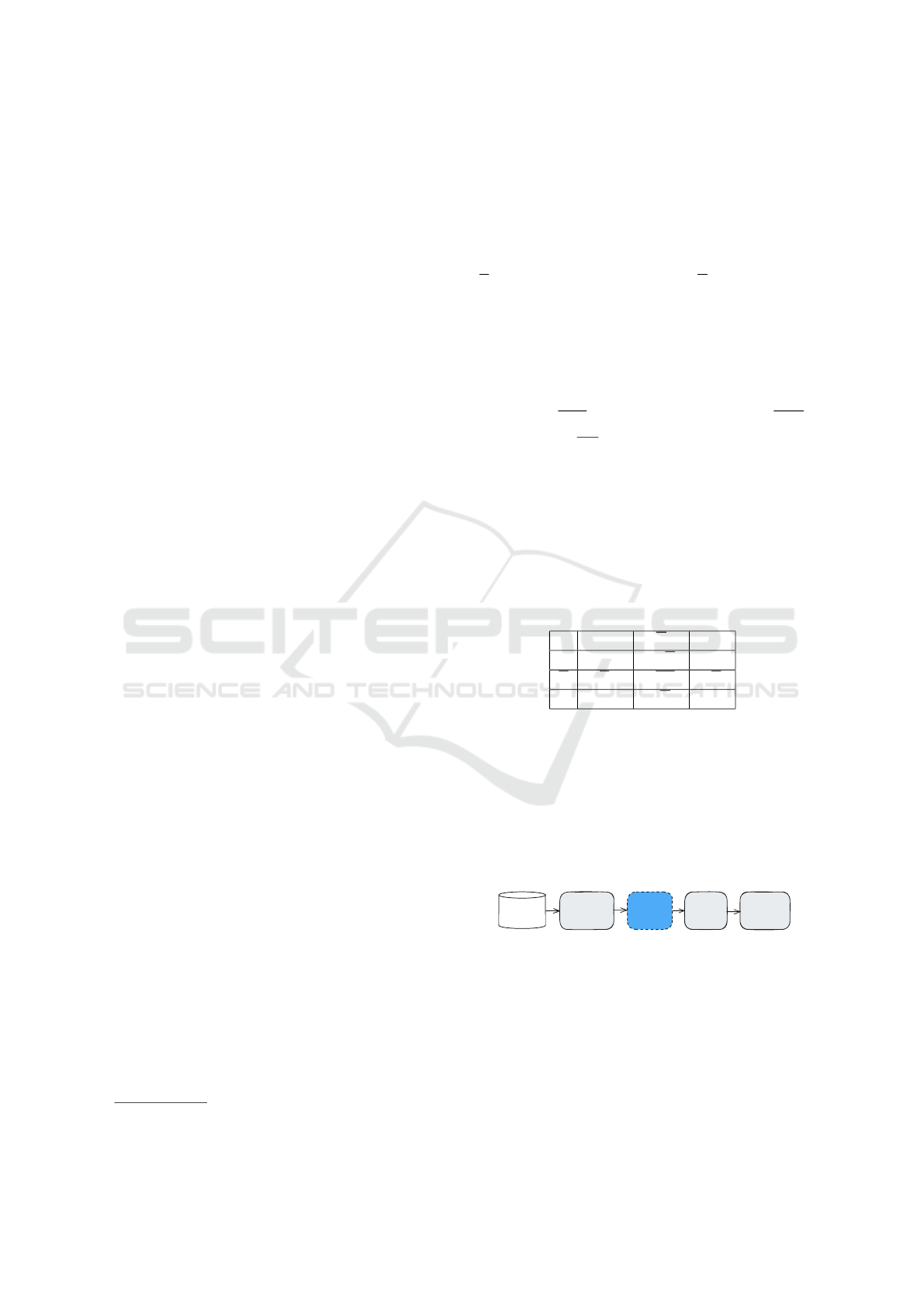
works. However, most AC algorithms perform
model induction in three or four steps, namely: [A]
Extraction, [B] Ranking and/or Pruning and [C]
Prediction, as seen in Figure 1. In CBA, these steps
work, broadly speaking, as follows:
Extraction Ranking Pruning Prediction
Database
Figure 1: Induction steps of an AC.
• Extraction: a modified version of Apriori
(Agrawal and Srikant, 1994) is run to obtain the
classification association rules (CARs).
• Ranking: given the set of CARs, the obtained
rules are ranked as follows: given two rules, r
i
and
r
j
, r
i
≻ r
j
, i.e., r
i
has higher precedence than r
j
if:
(i) the confidence of r
i
is greater than that of r
j
;
(ii) if the confidences are equal, but the support of
ICEIS 2025 - 27th International Conference on Enterprise Information Systems
318

B User's
Message
1 11 0
A User's
Message
1 10 0
C User's
Message
0 11 0
D User's
Message
1 01 0
E User's
Message
1 11 0
B User's
Message
1 11 0
h₁(K)
C User's
Message
D User's
Message
0 11 0
1 01 0
h₂(K)
h₃(K)
h₁(K+1)
Updated message
of B User
01 0
0
Update
Aggregate
Figure 2: Message passing mechanism in GNN. Extracted and Adapted from (Khemani et al., 2024).
r
i
is greater than the support of r
j
; (iii) confidence
and support are equal, but r
i
was generated before
r
j
. This ranking method is known as [CSC]
(Confidence, Support, Cardinality). This step is
highlighted in Figure 1, as it refers to the step
modified here, as well as in other works in the
literature presented below.
• Pruning: considering the obtained ranking,
pruning occurs as follows: for each rule r in the
ranked list it is checked the transactions it covers
and if it correctly covers at least one transaction.
In this case, the rule is selected to be included in
the model and all transactions covered by it are
removed from the dataset.
• Prediction: given an unseen object, the class label
associated with the first rule that matches the
object is the one to which it will be classified.
To evaluate the induced model, when dealing with
a classification task, evaluation measures are used
(Tan et al., 2019). This work used F1-Macro to assess
the performance of the models as in (Dall’Agnol and
Carvalho, 2024). Furthermore, to ensure a good
estimate, 10-fold stratified cross-validation was also
used, as in (Dall’Agnol and Carvalho, 2024). Another
important aspect used to assess rule-based models
is interpretability. According to (Margot and Luta,
2021) there is no exact mathematical definition for
this concept and, therefore, works evaluate this aspect
using different measures. This work used the number
of rules contained in the model (Model Size), as in
(Dall’Agnol and Carvalho, 2024). In this case, the
smaller the number of rules, the better the induced
model, i.e., the more interpretable it is.
Graph Convolutional Network (GCN). Among the
advantages of modeling a problem via graphs is
the feasibility of making explicit the relationships
(edges) that exist between the entities (nodes) in the
domain, making it possible to solve a task considering
both the topology of the network, i.e., the relational
context, and the descriptive attributes of the entities.
Through edges (relationships), algorithms can capture
information from the neighbors of a node, enabling
the learning of interactions that are difficult to model
with traditional representations.
Recently, due to their high effectiveness, graph
neural networks (GNNs) have been widely applied
in graph analysis (Zhou et al., 2020). According
to (Khemani et al., 2024), GNNs are a type
of deep learning model that uses a message
passing mechanism to aggregate information from
neighboring nodes, allowing them to capture complex
relationships. Figure 2 presents the general idea
of how the message passing mechanism works for
a given node. The messages to be passed are
represented by feature vectors. Therefore, given an
input graph with a set of node features (messages),
at each iteration k, each node collects topological
and feature information from the surrounding
neighborhood to update itself. In other words, at
each iteration, the neighbors of a node update its
feature vector by aggregating their information into
it. In the end, an embedding for each node is learned
based on the aggregated information. The left side of
Figure 2 presents a fictitious network. Each node is
a user described by a set of features (message). On
the right side, the aggregation and update operations
considering node-1 (User B) are illustrated. Since
this node is connected with node-2 (User C) and
node-3 (User D), their message (features) are sent
to node-1 and aggregated with its own message,
updating its embedding. In Figure 2, h
n
(k) indicates
an embedding h of a node n at iteration k (i.e., at layer
k).
Many GNN models are available today (Ju
et al., 2024), including the representative GCN
model proposed by (Kipf and Welling, 2017), being
one of the basic GNN variants and, therefore,
easy to implement and computationally efficient
(it presents fewer hyperparameters and a simpler
architecture). Furthermore, GCN excels in the context
of semi-supervised learning, where only a small
portion of the nodes are labeled and used to label,
via propagation, the rest of the unlabeled ones. The
Using Graph Convolutional Networks to Rank Rules in Associative Classifiers
319

Table 2: Set of OMs used by (Dall’Agnol and Carvalho, 2024).
Set OMs
[TW]
Support, Prevalence, K-Measure, Least Contradiction, Confidence, TIC, Leverage, DIR,
Loevinger, Odds Ratio, Added Value, Accuracy, Lift, J-Measure, Recall, Specificity,
Conditional Entropy, Coverage
[GF]
Odd Multiplier, Complement Class Support, Loevinger, Odds Ratio, Confidence Causal,
Confirmed Confidence Causal, J-Measure, Confidence
[C1]
Odd Multiplier, Complement Class Support, Confidence Causal, Loevinger, Added Value,
One Way Support, Confirmed Confidence Causal, Lift, Confidence, Putative Causal Dependence,
Leverage, Confirm Causal, TIC, DIR, Normalized Mutual Information
[G1]
Complement Class Support, Confidence, Confidence Causal, Confirmed Confidence Causal,
DIR, Loevinger, Odd Multiplier, TIC
[G2]
Added Value; Lift; One Way Support; Putative Causal Dependency
message passing in GCN is expressed mathematically
in Equation 1 (see (Kipf and Welling, 2017) for
details):
H
(k+1)
= σ(
˜
D
−
1
2
˜
A
˜
D
−
1
2
H
(k)
W
(k)
), (1)
where H
(k)
represents the matrix of activations in
the k
th
layer,
˜
A = A + I
N
the adjacency matrix of an
undirected graph G with added self-connections, I
N
the identity matrix,
˜
D
ii
=
∑
j
˜
A
i j
, W
(k)
a layer-specific
trainable weight matrix, and σ(.) an activation
function such as ReLU. For classification tasks, the
cross-entropy loss function is often used for training.
Therefore, the trained GCN model can be seen as
a function f (X, A), where X represents a matrix
of node feature vectors x
i
and A the adjacency
matrix that represents the graph G. Finally, the
learned embeddings from the final layer, i.e., H
(k)
,
are used to perform node classification, i.e.,
ˆ
Y =
σ(H
(k)
W
out
), where softmax is often used as σ(.) for
classification tasks, and W
out
are trainable weights to
map the embeddings to class probabilities. It is worth
mentioning that some hyperparameters need to the
defined to execute GCN, such as number of layers,
hidden units, activation functions, loss function,
among others. Therefore, the implementation used
here was based on the code created by (Kipf and
Welling, 2017).
AC.Rank
A
AC.Rank
A
AC.Rank
A
. Works have been proposed aiming to
modify the ACs ranking step since a large number
of OMs exists and none of them is suitable for all
explorations (Sharma et al., 2020). The idea is to use
a set of measures simultaneously to reduce the need
to choose a single measure, also considering different
aspects (semantics) for sorting the rules. One of
these works is AC.Rank
A
, presented in Figure 3. The
idea is to incorporate its ranking mechanism into
ACs induction flows aiming to induce models that
present a good balance between performance and
interpretability. The authors analyzed AC.Rank
A
in
different induction flows, comparing it when ranking
occurs via [CSC] (CBA sorting (baseline)). In
general, the AC.Rank
A
mechanism works as follows:
given a set of rules, a set of OMs is computed
for each of them. To do so, it is necessary to
specify the set of OMs to be used. The authors
explored 5 different sets, namely: [TW], [GF],
[C1], [G1] and [G2]. Table 2 presents the OMs
that make up each set, whose definitions (equations)
can be found in (Tew et al., 2014). Details about
the sets can be found in (Dall’Agnol and Carvalho,
2024)
3
, (Dall’Agnol and De Carvalho, 2023a) and
(Dall’Agnol and De Carvalho, 2023b). Based on the
selected set a “Rules” x “OMs” matrix is constructed
and used by one of the aggregation methods explored
by the authors, namely: [WS] (WSM), [WP] (WPM),
[TS] (TOPSIS), [BM] (Borda Arithmetic Mean),
[BD] (Borda Median), [BG] (Borda Geometric Mean)
and [BL] (Borda L2-norm). According to the authors,
the best combination is [GF]+[BL], and the one that
should actually be used. For this reason, in Section 4,
the method presented here will be compared to
AC.Rank
A
in this configuration. Basically, [BL]
computes the rank Rank
i
of each rule i as follows:
Rank
i
=
n
q
∑
n
j=1
Mat
2
i j
n
, where i indicates a rule, j an
OM, n the number of OMs and Mat
i j
the position of
rule i in a list ordered by an OM j (position i, j of the
matrix). After that, considering this new ranking, the
flow goes on, i.e., the rules are pruned and the model
is finalized aiming at the predictions.
MoMAC. Aiming to modify the ACs ranking step,
similarly as the AC.Rank
A
work, (Bui-Thi et al.,
2022) proposed MoMAC, presented in Figure 4.
The goal is to find a ranking that ensures a good
balance between performance, in this case estimated
by Accuracy, and interpretability. However, they do
not work directly with the OMs, but rather with the
probabilities that generate the measures. In general,
3
Regarding the [GF] group, in this reference the authors
forgot to remove the equivalent measures from the list.
ICEIS 2025 - 27th International Conference on Enterprise Information Systems
320

Ranking
Extraction
Pruning
Prediction
[GF] + [BL]
OM₁
OMₙ
Rₘ
...
...
R₁
Database
Figure 3: Ranking mechanism of AC.Rank
A
.
MoMAC works as follows: given a set of rules,
their contingency table, as in Table 1, are computed.
Based on the table of each rule, 15 probabilities are
considered and a “Rules” x “Probabilities” matrix
is constructed. The 15 probabilities are: P(A),
P(A), P(C), P(C), P(AC), P(AC), P(AC), P(AC),
P(A|C), P(A|C), P(A|C), P(A|C), P(C|A), P(C|A),
P(A)P(C). Then, given the matrix, a Multi-Layer
Perceptron (MLP) is trained using the probabilities
as input to predict a value (I(r)) for each rule that
will be used to rank them. In other words, the
network has to learn the right weights to generate
a ranking that will provide a model with a good
balance between performance and interpretability.
The predicted value (I(r)) is seen as the aggregation
of many “implicit” OMs, since all measures are
derived from the probabilities of the contingency
table. Since the weights are learned through a genetic
algorithm (NSGAII), the process is iterative, i.e., after
evaluating each individual in the population (a vector
of weights) through ranking, pruning and prediction,
the best individuals are selected, a new population is
generated and the flow starts again, using new weights
to generate new rankings and, therefore, new models,
until reaching a certain stopping criterion. At the
end, a two-dimensional graphic is presented to the
user so that he can choose the individual from the
final population that best balances, according to his
analysis, performance and interpretability.
3 AC.RANK
GCN
AC.RANK
GCN
AC.RANK
GCN
This section presents the method proposed here,
named AC.RANK
GCN
, which, like other literature
works, aims to modify the ranking step to obtain
models that present a good balance between
performance (F1-Macro) and interpretability (Model
Size) when a set of OMs is used simultaneously.
Ranking
...
...
MLP
Extraction
Pruning
Prediction
Database
P(A)
P(A|B)
Rₘ
...
...
R₁
Genetic Algorithm
W₁₁
W₁₂
Wᵢⱼ
...
Figure 4: Ranking mechanism of MoMAC.
However, the goal was to improve the results obtained
so far evaluating the importance of a rule not only
in relation to the values of its OMs, but also in
relation to its neighboring rules (neighborhood) and
their features. To this end, the problem was modeled
using a graph approach via semi-supervised learning,
in which the importance (rank) of each rule is a
label to be learned considering its neighborhood
and features. Since Graph Convolutional Networks
(GCNs) are applied in semi-supervised contexts and
take into account, during learning, both the network
topology and the node attributes, they were used
in this work. The proposal is a mix of ideas
from both previously described literature works, i.e.,
AC.Rank
A
and MoMAC. It is important to mention, as
already stated, that achieving a good balance between
performance and interpretability means improving
one of them without worsening the other in relation
to some baseline, since, as stated by (Dall’Agnol
and Carvalho, 2024), an inverse relationship between
them exists. Figure 5 presents AC.RANK
GCN
flow,
which is described below.
Matrices Generation. Given a set of rules, two
matrices are obtained: “Rules” x “OMs” (Mat.M),
as in (Dall’Agnol and Carvalho, 2024), and “Rules”
x “Probabilities” (Mat.P), as in (Bui-Thi et al.,
2022). However, in this case, 16 probabilities are
considered: P(A), P(A), P(C), P(C), P(AC), P(AC),
P(AC), P(AC), P(A|C), P(A|C), P(A|C), P(A|C),
P(C|A), P(C|A)
P(C|A)
P(C|A), P(C|A), P(C|A
P(C|A
P(C|A). In (Bui-Thi et al.,
2022) those highlighted in bold were not considered,
although they are variations of others considered,
and different from (Bui-Thi et al., 2022) we did
not consider P(A)P(C), since both probabilities were
already considered separately
4
. Regarding the OMs,
4
When P(AC) = P(A)P(C), A and C are statistically
independent, i.e., there is no relationship between the
Using Graph Convolutional Networks to Rank Rules in Associative Classifiers
321

Ranking
Extraction
Pruning
Prediction
Initial Ranking
R1
R2
R3
R5
R9
GCN
Database
OM₁
OMₙ
Rₘ
...
...
R₁
P(A)
P(A|B)
Rₘ
...
...
R₁
Figure 5: Ranking mechanism of AC.RANK
GCN
.
the sets [TW], [GF], [G1] and [G2] were explored,
as in (Dall’Agnol and Carvalho, 2024) (see Table 2).
Set [C1] was not used because it is a previous version
of sets [G1] and [G2].
Graph Construction. Based on the two matrices,
a graph is constructed. Each node in the graph
represents a rule, which is described by a set of
features extracted from Mat.P. Using Mat.M, each
edge represents the similarity between two rules
with respect to their set of OMs. However, edges
are only created between rules that present high
similarity (⩾ 99%)
5
, i.e., high agreement regarding
their ranks, since we assume that only nodes that
belong to the same class should be connected. The
similarity between two rules i and j is computed
by 1 −
∑
n
k=1
|Mat.M
ik
−Mat.M
jk
|
n
(normalized Manhattan),
where n indicates the number of OMs considered
and Mat.M
ik
the position of rule i in a list ordered
by an OM k (position i, k of Mat.M) (the same
for Mat.M
jk
). Therefore, it is possible to learn a
node representation (embedding) that considers, at
the same time, the graph structure (defined by a set
of OMs), the node features (described by a set of
probabilities) and neighborhood information.
Labeling. As mentioned, the problem was modeled
via semi-supervised learning. The idea is that GCN
learns the embeddings of each rule (node) considering
the importance (class) of some initial rules. Since
occurrences of A and C (Tan et al., 2019). On the other
hand, when P(AC) > P(A)P(C), A and C are positively
correlated; otherwise, negatively correlated (Tan et al.,
2019). Thus, we did not consider P(A)P(C) in the list
of probabilities, since we assumed that the information is
implicit through P(AC), P(A) and P(C).
5
This similarity threshold could be a hyperparameter
(HyP-1) to be better explored in the future.
R₁
...
R₂ ...R₉ Rₘ
R₁
...
...
R₂
...
RₘR₉
...
R₁
...
R₂
...
RₘR₉
...
...
Ranking: [OMs Set] + [BL]
Slit by bins and Class definition
Random selection of nodes
R₁
R₂
Rₘ
R₉
Figure 6: Labeling step.
embeddings encode for each node both the aggregated
features of its neighbors and the graph structure, it
is possible to identify the importance of each rule
considering not only its values in a set of OMs, but
also these values in relation to its neighboring rules
and the attributes that describe them, that is, their
expanded contingency matrices. As the class of any
rule is not known at this point, a labeling is performed
considering an initial ranking of the rule set. The
labeling works as described below (Figure 6):
• Given the set of rules, a ranking is generated.
The ranking is done as described in (Dall’Agnol
and Carvalho, 2024)’s work, depending on the
set of OMs used in the Graph Construction
step (Mat.M). Regardless of the set, the [BL]
aggregation method is used, as it has proven to
be stable across the sets of measures.
• Based on the ranking generated, the rules, now
sorted, are divided into 20
6
bins of equal size
(such as equal width), so that the rules contained
in the first bin are considered as belonging to
class 1 (label 1), those in the second bin to class
2 (label 2), and so on. Thus, rules belonging
to the first classes (first bins) are more relevant
than those belonging to the final classes (last
bins). After that, 20%
7
of the rules are randomly
selected to identify the nodes that will be labeled
according to the classes defined via bins so
that the embeddings are learned and the label
propagation is performed. It is possible that a
certain class may be left out, since the selection
6
The number 20 was chosen experimentally to avoid
generate an excessively large number of classes. However,
this may be a hyperparameter (HyP-2) to be better explored
in future work.
7
This percentage was chosen experimentally,
representing the proportion of labeled nodes. However, this
may be a hyperparameter (HyP-3) to be better explored in
future work.
ICEIS 2025 - 27th International Conference on Enterprise Information Systems
322

of rules is done randomly. However, in this case,
this does not pose a problem, as the labels are
actually pseudo-labels, which are used to direct
the learning of the embeddings.
Label Prediction. Based on the labels previously
defined, GCN is trained to find the labels of the
unlabeled nodes based on the learned embeddings.
The idea is to find the importance of each rule not only
in relation to a set of measures, but also in relation to
its neighbors, that are described by a set of features.
Ranking. After training, unlabeled nodes are labeled
as belonging to the highest probability class in their
output embedding. Given that each rule is then
labeled, their ranking is performed as follows: the
rules are ordered from the best class to the worst class
and among the rules of the same class, priority is
given to those with the highest support value (as in
the CBA tiebreaker criterion).
Finally, as in other works, after modifying the
ranking step, the induction flow continues until
prediction. It is noticed that the proposed method can
be seen as a mixture of previous works available in
the literature aiming to obtain better results.
4 EXPERIMENTS, RESULTS AND
DISCUSSION
Experiments were carried out to evaluate the method
proposed here (AC.RANK
GCN
). For that, as in
(Dall’Agnol and Carvalho, 2024), CBA was used
as baseline, i.e., we changed the CBA ranking step
by AC.RANK
GCN
and compared it with CBA to
verify whether the induced models presented a better
balance between performance and interpretability.
We also compared AC.RANK
GCN
with AC.Rank
A
instantiated with [GF]+[BL], since (Dall’Agnol and
Carvalho, 2024) demonstrated its best result in
relation to CBA; on the other hand, MoMAC was
not considered, as it does not achieve good results
according to the authors.
To execute CBA, AC.Rank
A
and AC.RANK
GCN
,
some requirements are needed. Regarding the
datasets, their treatments (pre-processing) and aspects
related to rule extraction, we used the configurations
as described in (Dall’Agnol and Carvalho, 2024),
aiming to guarantee a fair comparison between the
works. However, among the 43 datasets presented in
(Dall’Agnol and Carvalho, 2024), 41 were used
8
, as 2
of them were disregarded because they produced less
than 100 rules, making it difficult to apply the method
proposed here.
8
https://bit.ly/gcn-datasets.
Regarding AC.RANK
GCN
, it was executed with
the following configurations: [TW;TW+BL],
[GF;GF+BL], [G1;G1+BL] and [G2;G2+BL]. The
notation before the “;” refers to the set of OMs in
Mat.M used in the construction of the graph (“Graph
Construction” step). The notation after the “;”
refers to the way of obtaining the ranking to define
the labels (“Labeling” step). Regarding the GCN
hyperparameters (HyP-GCN), we used the same
configurations described in (Kipf and Welling, 2017)
(activation functions, loss function, etc.), except for
the number of layers, which was set to 1, and the
number of hidden units, which were set to 32, since
the features vector has dimension 16. As mentioned
before, the implementation was based on the code
9
created by (Kipf and Welling, 2017).
Regarding the evaluation criteria, the measures
considered were F1-Macro, in terms of performance,
and Model Size, in terms of interpretability, both
estimated through 10-fold stratified cross-validation.
Furthermore, to compare the obtained results,
statistical tests were carried out using the Friedman
test with α = 0.05 and the Nemenyi post-hoc test
(Friedman+Nemenyi), together with the critical
difference (CD) diagrams, as recommend by
(Demsar, 2006). Therefore, a total of 2,460
experiments were executed (6 flows × 41 datasets ×
10-fold cross-validation).
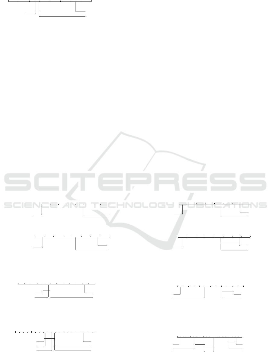
Figures 7 to 10 present the results. Each CD
diagram
10
refers to the average results
11
obtained by
the methods on the 41 datasets with respect to an
evaluation measure (F1-Macro or Model Size) over
the 10-folds. It is possible to notice that:
• regarding performance (F1-Macro), the Friedman
test did not detect a difference between
AC.RANK
GCN
(GCN for short) executed with
[GF;GF+BL], [G1;G1+BL] and [G2;G2+BL]
in relation to AC.Rank
A
and CBA (the null
hypothesis was not rejected (p-values
∼
=
0.21, 0.07
and 0.15 respectively). However, GCN executed
with [TW;TW+BL] presented a statistical
difference and, therefore, the post-hoc Nemenyi
test was applied along with a CD diagram, as
shown in Figure 7. Therefore, although GCN
was able to maintain the performance of the
models in the [GF;GF+BL], [G1;G1+BL]
and [G2;G2+BL] configurations, in the
[TW;TW+BL] configuration the performance
was below the baselines, not being an interesting
configuration to be used;
9
https://github.com/tkipf/gcn.
10
For more details on CD diagrams see (Demsar, 2006).
11
Available in https://bit.ly/results-acrankgcn.
Using Graph Convolutional Networks to Rank Rules in Associative Classifiers
323

1 2 3
CBA
AC.Rank.A
GCN[TW;TW+BL]
Figure 7: CD diagram between AC.RANK
GCN
and baselines
(AC.Rank
A
and CBA) regarding performance (F1-Macro) in
[TW;TW+BL] configuration.
• regarding interpretability (Model Size), all GCN
configurations presented a statistically significant
difference in relation to AC.Rank
A
and CBA. In
this case, a diagram was generated for each set
of OMs, as seen in Figure 8. In all of them
it is clear that GCN outperforms AC.Rank
A
and
CBA. Therefore, considering both performance
and interpretability, the only configuration that
does not perform well is [TW;TW+BL];
• comparing all GCN configurations (Figure 9), it
is possible to notice that regarding F1-Macro,
[TW;TW+BL] is the only configuration that
differs from the others, presenting a worse
performance (Figure 9a). On the other hand, it
is the best configuration regrading interpretability
(Figure 9b). As stated by (Dall’Agnol and
Carvalho, 2024), there is an inverse relationship
between performance and interpretability. Since
the aim here is to achieve a balance between
both, it can be noticed that [G2;G2+BL] is the
most suitable GCN configuration: it appears in
the second position of the first group regarding
F1-Macro (Figure 9a) and is the second best
option regarding interpretability (Figure 9b).
Therefore, AC.RANK
GCN
achieves its aim with
this configuration;
• comparing all GCN configurations with the
baselines (Figure 10), it is possible to notice
that, in fact, [G2;G2+BL] is the configuration
that guarantees a better balance between
performance and interpretability, since it
maintains performance (Figure 10a), but
improves interpretability (Figure 10b) in relation
to baselines.
5 CONCLUSION
This work presented a method (AC.RANK
GCN
) for
ranking rules in ACs induction flows. The aim is to
induce models that present a good balance between
performance (F1-Macro) and interpretability (Model
Size) when a set of OMs is used simultaneously.
The method mixes ideas from previous literature
works (AC.Rank
A
and MoMAC) to improve the
results obtained so far. The method uses a graph
convolutional network (GCN) in a semi-supervised
approach. The idea is to evaluate the importance
of a given rule considering its neighboring rules
1 2 3
GCN[TW;TW+BL]
AC.Rank.A
CBA
(a) [TW].
1 2 3
GCN[GF;GF+BL]
AC.Rank.A
CBA
(b) [GF].
1 2 3
GCN[G1;G1+BL]
AC.Rank.A
CBA
(c) [G1].
1 2 3
GCN[G2;G2+BL]
AC.Rank.A
CBA
(d) [G2].
Figure 8: CD diagram between AC.RANK
GCN
and baselines (AC.Rank
A
and CBA) regarding interpretability (Model Size).
1 2 3 4
GCN[G1;G1+BL]
GCN[G2;G2+BL] GCN[GF;GF+BL]
GCN[TW;TW+BL]
(a) F1-Macro.
1 2 3 4
GCN[TW;TW+BL]
GCN[G2;G2+BL] GCN[GF;GF+BL]
GCN[G1;G1+BL]
(b) Model Size.
Figure 9: CD diagram between AC.RANK
GCN
configurations.
1 2 3 4 5 6
AC.Rank.A
CBA
GCN[G1;G1+BL] GCN[G2;G2+BL]
GCN[GF;GF+BL]
GCN[TW;TW+BL]
(a) F1-Macro.
1 2 3 4 5 6
GCN[TW;TW+BL]
GCN[G2;G2+BL]
GCN[GF;GF+BL] GCN[G1;G1+BL]
AC.Rank.A
CBA
(b) Size.
Figure 10: CD diagram between AC.RANK
GCN
configurations and baselines (AC.Rank
A
and CBA).
ICEIS 2025 - 27th International Conference on Enterprise Information Systems
324

(neighborhood), the network topology and a set
of features that describe them. The method
outperformed AC.Rank
A
and CBA in terms of
interpretability while maintaining the performance of
the models. The best results were achieved with
[G2;G2+BL] configuration.
We believe that this study presents promising
results, which can be better explored in future works
regarding (i) the impact of hyperparameters on
the process (HyP-1, HyP-2, HyP-3, HyP-GCN),
(ii) the possibility of using GCNs in other steps
of the induction process, as well as in other
flows (as explored by (Dall’Agnol and Carvalho,
2024)), (iii) the construction of solutions that
incorporate black-box approaches to improve
inherently interpretable (white-box) solutions.
ACKNOWLEDGEMENTS
This study was financed in part by the Coordenac¸
˜
ao
de Aperfeic¸oamento de Pessoal de N
´
ıvel Superior
- Brasil (CAPES). The authors are also grateful to
the S
˜
ao Paulo Research Foundation - FAPESP (grant
#2024/04890-5) and the Brazilian National Council
for Scientific and Technological Development - CNPq
(grants #313193/2023-1 and #422667/2021-8) for
their financial support.
REFERENCES
Agrawal, R. and Srikant, R. (1994). Fast algorithms
for mining association rules in large databases. In
Proceedings of the 20th International Conference on
Very Large Data Bases (VLDB), pages 487––499.
Morgan Kaufmann Publishers Inc.
Bui-Thi, D., Meysman, P., and Laukens, K. (2022).
MoMAC: Multi-objective optimization to
combine multiple association rules into an
interpretable classification. Applied Intelligence,
52(3):3090––3102.
Dall’Agnol, M. and Carvalho, V. O. (2024). AC.RankA:
Rule ranking method via aggregation of objective
measures for associative classifiers. IEEE Access,
12:88862–88882.
Dall’Agnol, M. and De Carvalho, V. O. (2023a). Clustering
the behavior of objective measures in associative
classifiers. In 18th Iberian Conference on Information
Systems and Technologies (CISTI), pages 1–6.
Dall’Agnol, M. and De Carvalho, V. O. (2023b). Ranking
rules in associative classifiers via borda’s methods. In
18th Iberian Conference on Information Systems and
Technologies (CISTI), pages 1–6.
Demsar, J. (2006). Statistical comparisons of classifiers
over multiple data sets. J. Mach. Learn. Res., 7:1––30.
Ju, W., Fang, Z., Gu, Y., Liu, Z., Long, Q., Qiao, Z., Qin,
Y., Shen, J., Sun, F., Xiao, Z., Yang, J., Yuan, J.,
Zhao, Y., Wang, Y., Luo, X., and Zhang, M. (2024).
A comprehensive survey on deep graph representation
learning. Neural Networks, 173:106207.
Khemani, B., Patil, S., Kotecha, K., and Tanwar, S.
(2024). A review of graph neural networks: concepts,
architectures, techniques, challenges, datasets,
applications, and future directions. J Big Data,
11(18).
Kipf, T. N. and Welling, M. (2017). Semi-supervised
classification with graph convolutional networks.
In International Conference on Learning
Representations (ICLR).
Liu, B., Hsu, W., and Ma, Y. (1998). Integrating
classification and association rule mining. In In
Proceedings of the 4th International Conference on
Knowledge Discovery and Data Mining (KDD),,
pages 27–31.
Margot, V. and Luta, G. (2021). A new method to compare
the interpretability of rule-based algorithms. Ai,
2(4):621–635.
Rudin, C. (2019). Stop explaining black box machine
learning models for high stakes decisions and use
interpretable models instead.
Sharma, R., Kaushik, M., Peious, S. A., Yahia, S. B.,
and Draheim, D. (2020). Expected vs. Unexpected:
Selecting right measures of interestingness. In Big
Data Analytics and Knowledge Discovery - 22nd
International Conference (DaWaK), volume 12393,
pages 38–47.
Somyanonthanakul, R. and Theeramunkong, T. (2022).
Scenario-based analysis for discovering relations
among interestingness measures. Information
Sciences, 590:346–385.
Tan, P.-N., Steinbach, M., Karpatne, A., and Kumar, V.
(2019). Introduction to Data Mining. 2 edition.
Tew, C., Giraud-Carrier, C., Tanner, K., and Burton,
S. (2014). Behavior-based clustering and analysis
of interestingness measures for association rule
mining. Data Mining and Knowledge Discovery,
28(4):1004–1045.
Zhou, J., Cui, G., Hu, S., Zhang, Z., Yang, C., Liu, Z.,
Wang, L., Li, C., and Sun, M. (2020). Graph neural
networks: A review of methods and applications. AI
Open, 1:57–81.
Using Graph Convolutional Networks to Rank Rules in Associative Classifiers
325