Sleep-Stage Efficient Classification Using a Lightweight Self-Supervised
Model
Eldiane Borges dos Santos Dur
˜
aes and Jo
˜
ao Batista Florindo
a
Institute of Mathematics, Statistics and Scientific Computing, University of Campinas, Street Sergio Buarque de Holanda,
651, Campinas, Brazil
fl
Keywords:
Sleep-Stage Classification, mulEEG, Self-Supervised Learning, Linear SVM, EEG Signal.
Abstract:
Background and Objective: Accurate classification of sleep stages is crucial for diagnosing sleep disorders
and automating this process can significantly enhance clinical assessments. This study aims to explore the
use of a self-supervised model (more specifically, an adapted version of mulEEG) combined with a Linear
SVM classifier to improve sleep stage classification. Methods: The mulEEG model, which learns electroen-
cephalogram signal representations in a self-supervised manner, was simplified here by replacing ResNet-50
with 1D-convolutions used as time series encoder by a ResNet-18 backbone. Two other adaptations were
conducted: the first one evaluated different configurations of the model and data volume for training, while
the second tested the effectiveness of time series features, spectrogram features, and their concatenation as
inputs to a Linear SVM classifier. Results: The results showed that reducing the volume of data offered a
better cost-benefit ratio compared to simplifying the model. Using the concatenated features with ResNet-18
also outperformed the linear evaluations of the original mulEEG model, achieving higher classification perfor-
mance. Conclusions: Simplifying the mulEEG model to extract features and pairing it with a robust classifier
leads to more efficient and accurate sleep stage classification. This approach holds promise for improving
clinical sleep assessments and can be extended to other biological signal classification tasks.
1 INTRODUCTION
In the human body, sleep is divided into cycles, each
consisting of two distinct phases: Rapid Eye Move-
ment (REM) and Non-Rapid Eye Movement (NREM)
sleep, which is further divided into stages N1, N2, and
N3 (Patel et al., 2024). Each phase is characterized
by variations in muscle tone, brain wave patterns, and
eye movements. Furthermore, the human body un-
dergoes each sleep cycle 4 to 6 times per night, with
each cycle lasting approximately 90 minutes. How-
ever, sleep quality and time spent at each stage can
be affected by sleep-related or mental disorders, such
as obstructive sleep apnea, depression, schizophre-
nia, and dementia, as well as traumatic brain injuries,
medications, and circadian rhythm disorders. As a re-
sult, the identification of sleep stages plays a crucial
role in the diagnosis of these conditions, and automat-
ing this classification can significantly improve clini-
cal sleep assessments.
The mulEEG model described in (Kumar et al.,
2022) is an example of a modern successful ap-
a
https://orcid.org/0000-0002-0071-0227
proach in the deep learning category. It aims to auto-
mate the classification of sleep stages using electroen-
cephalogram (EEG) signals collected during sleep.
To achieve this, it performs a pretext task, which in-
volves learning effective representations of these EEG
signals from multiple data views in a self-supervised
manner. Despite the great results achieved by the
mulEEG model in ideal scenarios, with large amounts
of data and computational resources for pretraining,
we notice that the literature still lacks self-supervised
architectures adapted for contexts where the availabil-
ity of data and computational power is limited.
In this context, and inspired by self-supervised
models for time series analysis like mulEEG, here
we propose a self-supervised deep learning frame-
work for the identification of sleep stages. We take
mullEEG as our starting point, but leverage it with
strategies aiming at offering alternatives to simplify
both the model and its training process, while also
maximizing the utility of the learned representations
by using them as input to a Linear SVM algorithm for
the classification task.
The first strategy involves replacing ResNet-50
972
Durães, E. B. S. and Florindo, J. B.
Sleep-Stage Efficient Classification Using a Lightweight Self-Supervised Model.
DOI: 10.5220/0013367900003912
Paper published under CC license (CC BY-NC-ND 4.0)
In Proceedings of the 20th International Joint Conference on Computer Vision, Imaging and Computer Graphics Theory and Applications (VISIGRAPP 2025) - Volume 2: VISAPP, pages
972-979
ISBN: 978-989-758-728-3; ISSN: 2184-4321
Proceedings Copyright © 2025 by SCITEPRESS – Science and Technology Publications, Lda.

with 1D-convolutions in the time series encoder with
a ResNet-18, and alternating the usage of the pretext
dataset between 20% and 100%. The second one in-
volves several training of the Linear SVM using the
representations learned by the self-supervised module
with either ResNet-50 or ResNet-18, which are the
time series features, spectrogram features, and their
concatenation.
To assess the performance of the proposed model,
the main evaluation metrics were accuracy (Acc), Co-
hen’s kappa (κ), and macro-averaged F1 score (MF1).
The reference for comparison was the linear evalu-
ation of mulEEG presented in (Kumar et al., 2022),
where a linear classifier was trained using only the
time series features as input. However, the training of
the Linear SVM with the concatenation of both fea-
tures learned by mulEEG using ResNet-18 was suffi-
cient to surpass the results reported in (Kumar et al.,
2022).
2 RELATED WORKS
As stated in (Sekkal et al., 2022), the methods
used to automate the classification of sleep stages
are based on two main strategies: (i) conven-
tional machine learning methods and (ii) deep learn-
ing approaches based on artificial neural networks.
The first category includes algorithms such as K-
Nearest Neighbors (KNN), Support Vector Machines
(SVM), Random Forests (RF), Decision Trees, and
Bayesian rule-based classifiers. The second cate-
gory comprises Multi-Layer Perceptrons (MLP) and
their modern refinements, including Recurrent Neural
Networks (RNNs), Long Short-Term Memory Net-
works (LSTMs), Gated Recurrent Units (GRUs), Bi-
directional LSTMs, and Convolutional Neural Net-
works (CNNs). Our study lies in the second category.
A recent review on deep learning techniques used for
sleep stage classification can be found in (Liu et al.,
2024).
Deep learning can be further divided into differ-
ent learning paradigms, such as supervised, unsuper-
vised, and, more recently, self-supervised learning.
This last group is particularly interesting in scenar-
ios where the access to annotated data for training
is limited. Several works have investigated the use
of self-supervised learning on EEG signals, for ex-
ample, the study in (Xiao et al., 2024), where an
algorithm based on contrastive learning is used for
seizure detection. Specifically on sleep stage clas-
sification, we have (Eldele et al., 2023), which pro-
vides a systematic evaluation of SSL in few-label set-
tings. The authors in (Yuan et al., 2024) opt for an-
alyzing non-polysomnography data, particularly ac-
quired by wrist-worn accelerometers. In our study,
we focus specifically on mulEEG approach (Kumar
et al., 2022), considering the richness of the deep EEG
representation that the model provides by combining
SSL with a multi-view description. We differentiate
from the original model with respect to the focus on
computational efficiency and in solving a real-world
task, which is classification, instead of feature repre-
sentation learning, which is the focus in (Kumar et al.,
2022).
3 BACKGROUND
In this section, the fundamental elements to be used
in our methodology are described. They are the
mulEEG, a multi-view representation learning model
on EEG signals (Kumar et al., 2022), and the Lin-
ear Support Vector Machine (Bishop and Nasrabadi,
2006), which is chosen here as the classification head.
3.1 mulEEG
The mulEEG model, presented in (Kumar et al.,
2022), is a self-supervised multi-view method to learn
the representation of EEG signals. The objective
is to effectively utilize the complementary informa-
tion of the EEG multi-view signals. Also, this self-
supervised method follows the contrastive learning
approach.
In order to obtain the multi-view of EEG signals,
first data augmentation is applied. The family of aug-
mentations T
1
uses jittering, in which uniform noise
is added to the EEG signal, and masking, in which
signals are masked randomly, ending up with the time
series t
1
. On the other hand, in the family of aug-
mentations T
2
, the EEG signals are randomly flipped
in horizontal direction and then scaled with Gaussian
noise, resulting in the time series t
2
. Additionally,
t
1
and t
2
are converted into their respective spectro-
grams, s
1
and s
2
, by a Short-Time Fourier Transform
S. In this way, we have all the EEG signal views to be
used.
Thereby, the mulEEG model is composed by the
time series encoder E
t
, which is a ResNet-50 with 1D
convolutions, and the spectrogram encoder E
s
as fea-
ture extractors. They are responsible for obtaining the
effective EEG signal representations.
Once the time series and spectrogram features
have been obtained, they are passed into projection
heads, which map those representations to the space
where the contrastive loss will be applied. This struc-
ture is a fully connected neural network whose layer
Sleep-Stage Efficient Classification Using a Lightweight Self-Supervised Model
973

sequence corresponds to: Linear, Batch Norm, ReLU,
and Linear. For each family of augmentations T
i
,
i = 1,2, there are three projection heads, one for each
kind of feature: time series ( f
i
), spectrogram (h
i
),
and the concatenation of both (g
i
). The correspond-
ing contrastive losses are named L
T T
, L
SS
, and L
FF
,
which gives more flexibility to optimize each feature.
The diagram of mulEEG is presented in Figure 1.
The model employs a variant of contrastive loss
called NT-Xent, which maximizes the similarity be-
tween two augmented views while minimizing its
similarity with other samples (Kumar et al., 2022),
given by Equation (2). Notice that N is the batch size,
τ is the temperature parameter, and cosine similarity
is used.
l(i, j) = −log
exp(cos(z
i
,z
j
)/τ)
∑
2N
k=1
I
[k̸=i]
exp(cos(z
i
,z
k
)/τ)
!
,
(1)
L(z
i
,z
j
) =
1
2N
N
∑
k=1
l(2k − 1,2k) + l(2k,2k − 1). (2)
We also have the diverse loss L
D
, which forces the
complementary information between time series and
spectrogram views. This loss is applied over the time
series and spectrogram features from both families of
augmentations of a single sample instead of the entire
batch, ignoring the concatenated features, which tend
to maximize the mutual information between those
features. The diverse loss is represented in Equation
(4), where z
k
= [z
t
i
,z
t
j
,z
s
i
,z
s
j
] is taken with respect to
a single sample and τ
d
is the temperature parameter.
The total loss, a linear combination of all the losses
previously described with parameters λ
1
and λ
2
, is
represented by Equation 5.
l
d
(z
k
,a,b) = − log

exp(cos(z
k
[a],z
k
[b])/τ
d
)
∑
4
i=1
I
[i̸=a]
exp(cos(z
k
[a],z
k
[i])/τ
d
)

,
(3)
L
D
=
1
4N
∑
N
k=1
l
d
(z
k
,1,2) +l
d
(z
k
,2,1) +l
d
(z
k
,3,4) +l
d
(z
k
,4,3),
(4)
L
tot
= λ
1
(L
T T
+ L
FF
+ L
SS
) + λ
2
L
D
. (5)
For the final outcome of the model, the pre-trained
encoders are submitted to a linear layer, which is at-
tached right after the frozen time series encoder and
only this specific layer is trained, evaluating the cho-
sen metrics as shown in Figure 2. Therefore, mulEEG
does not explore the sleep-stage classification task but
learns effective representations of it.
3.2 Linear SVM
Support Vector Machine (SVM) is a supervised ma-
chine learning algorithm that can be used in binary
classification problems. The SVM goal is to obtain
the maximum margin that separates hyperplanes cor-
responding to decision boundaries over the classes.
Next, the Linear SVM description is presented ac-
cording to (Pedregosa et al., 2011).
Given a sample (x, y), with input vector x ∈ R
n×1
and label y ∈ {−1, 1}, consider the prediction given
by (w
T
x+b), where w ∈ R
n×1
is the weight and b ∈ R
is the bias term. The hinge loss used in Linear SVM
can be defined as
max(0,1 − y(w
T
x + b)). (6)
Note that if the prediction is correct, the hinge loss is
equal to zero.
Thereby, given m samples {(x
(i)
,y
(i)
)}
m
i=1
, the
Linear SVM solves the following problem:
argmin
w,b
C
m
∑
i=1
max(0,1 −y
(i)
(w
T
x
(i)
+ b))+
1
2
w
T
w
!
.
(7)
In Equation (7), a regularization term is included via
C > 0, which acts as the inverse of the regularization
penalty.
One can also increase the complexity of SVM by
the addition of a kernel function, which transforms the
input vectors in such a way that the class separation is
performed by complicated non-linear decision bound-
aries. However, in the Linear SVM, the kernel func-
tion is the identity. Additionally, in a multi-class clas-
sification problem, strategies like “one-vs-the-rest” or
“one-vs-one” can be applied.
4 PROPOSED METHOD
Taking into consideration that, despite its effective-
ness in EEG analysis, mulEEG is a complex model
and its training algorithm has a high computational
cost, the proposed method adapts the original archi-
tecture, with the objective of obtaining similar ac-
curacy with a singnificantly reduced computational
overhead. In a first stage, we substitute the ResNet-
50 in the time series encoder by a ResNet-18, also us-
ing 1D-convolutions. This adaptation aims to verify
whether a simpler model can also be effective in the
classification task. The amount of data used to train
the model was also varied to check the need for a large
dataset for this task. The architectures for ResNet-50
and ResNet-18 with 1D convolutions in the encoder
E
t
are presented in Tables 1 and 2, respectively. The
architecture of the ResNet-18 was adapted with 1D-
convolutions based on (He et al., 2015).
Additionally, once the EEG signal representations
were learned, a Linear SVM is trained for sleep-stage
classification. This step has the goal of checking how
VISAPP 2025 - 20th International Conference on Computer Vision Theory and Applications
974

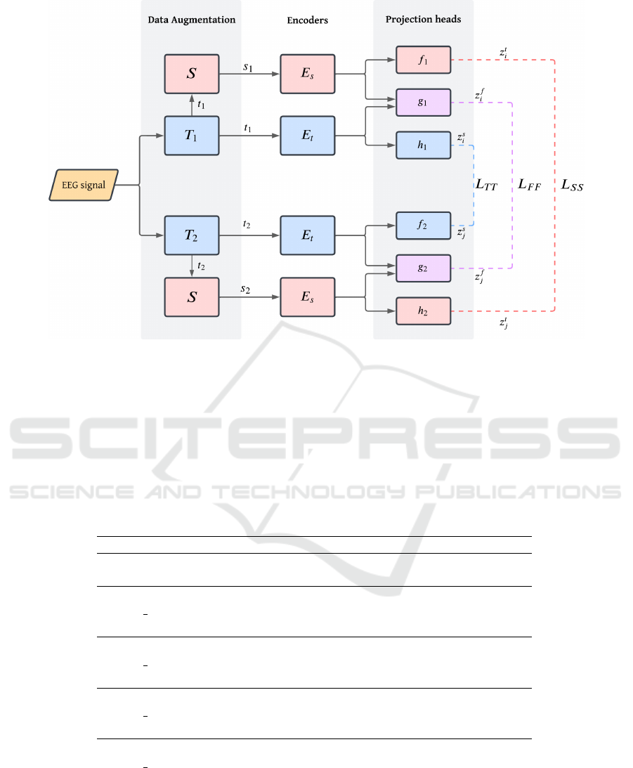
Figure 1: MulEEG structure. First, the EEG signal goes through data augmentation, in which we get the time series views
of the families of augmentations T
1
and T
2
and their conversions to spectrograms by the Short Time Fourier Transform
S. Then, these views are passed to encoders E
t
for time series and E
s
for spectrograms. Finally, the outputs go through
distinct projection heads depending on the type of view (time series, spectrogram or their concatenation) and the family of
augmentations, where the contrastive loss is applied between the projections of the same type.
Table 1: Architecture of ResNet-50 with 1D-convolutions used in mulEEG. Consider the input dimension as [256× 1 ×3000],
where 256 is the batch size, 1 is the number of channels, and 3000 is the length of each sample. The residual blocks are
represented in brackets and their numbers of repetition are indicated at right. Additionally, k is the kernel size, f is the
number of filters, s is the stride, and p is the padding of the 1D-convolution. Notice that s = 2 means that the stride is
actually equal to 2 only in the first repetition of the corresponding bottleneck block, so there is a down-sampling. In the next
repetitions, the stride is equal to 1.
ResNet-50 with 1D-convolutions used in mulEEG.
Layer Output dimension Architecture
Conv0
[256 × 16 × 1500] k = 71, f = 16, s = 2, p = 35
[256 × 16 × 750] k = 71, s = 2, p = 35 Max-Pooling
Conv1 x [256 × 32 × 750]


k = 1 f = 8 s = 1 p = 0
k = 25 f = 8 s = 1 p = 12
k = 1 f = 32 s = 1 p = 0


× 3
Conv2 x [256 × 64 × 375]


k = 1 f = 16 s = 1 p = 0
k = 25 f = 16 s = 2 p = 12
k = 1 f = 64 s = 1 p = 0


× 4
Conv3 x [256 × 128 × 188]


k = 1 f = 32 s = 1 p = 0
k = 25 f = 32 s = 2 p = 12
k = 1 f = 128 s = 1 p = 0


× 6
Conv4 x [256 × 256 × 94]


k = 1 f = 64 s = 1 p = 0
k = 25 f = 64 s = 2 p = 12
k = 1 f = 256 s = 1 p = 0


× 3
effective those features are in a more robust classifi-
cation algorithm, since the baseline architecture had
a simple linear classifier to provide its output. The
choice of using a linear kernel on SVM is justified by
the huge data volume used in the experiments. Ac-
cording to (Pedregosa et al., 2011), an SVM with
non-linear kernel scales at least quadratically with the
number of samples, while the SVM with linear ker-
nel can scale almost linearly to millions of samples.
Thereby, the Linear SVM is a sufficient algorithm for
Sleep-Stage Efficient Classification Using a Lightweight Self-Supervised Model
975

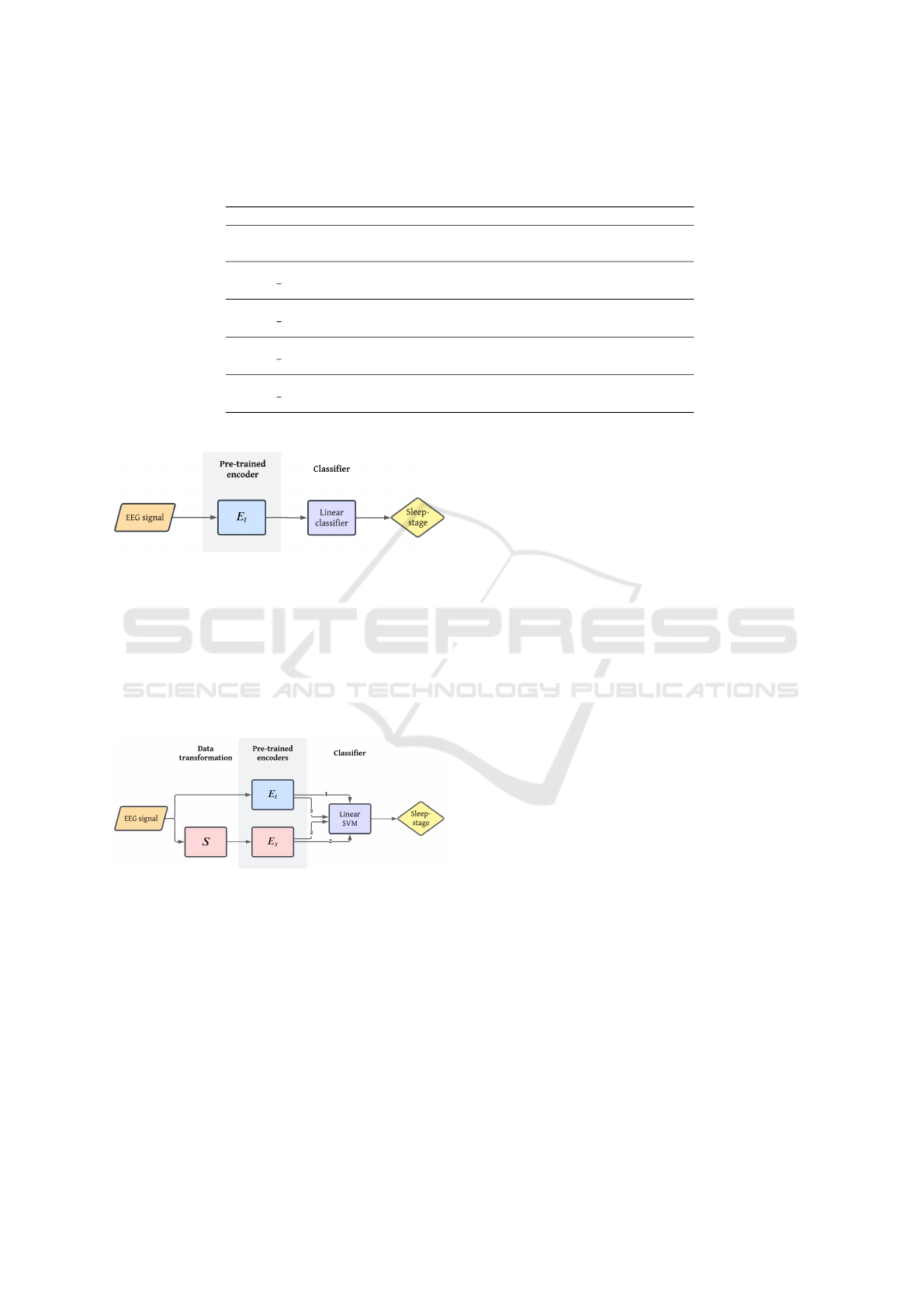
Table 2: Architecture of the ResNet-18 adapted in our method with 1D-convolutions. The notation is identical to that in Table
1.
ResNet-18 adapted with 1D-convolutions
Layer Output dimension Architecture
Conv0
[256 × 16 × 1500] k = 71, f = 16, s = 2, p = 35
[256 × 16 × 750] k = 71, s = 2, p = 35 Max-Pooling
Conv1 x [256 × 8 × 750]

k = 25 f = 8 s = 1 p = 12
k = 25 f = 8 s = 1 p = 12

× 2
Conv2 x [256 × 16 × 375]

k = 25 f = 16 s = 1 p = 12
k = 25 f = 16 s = 2 p = 12

× 2
Conv3 x [256 × 32 × 188]

k = 25 f = 32 s = 1 p = 12
k = 25 f = 32 s = 2 p = 12

× 2
Conv4 x [256 × 64 × 94]

k = 25 f = 64 s = 1 p = 12
k = 25 f = 64 s = 2 p = 12

× 2
Figure 2: Linear evaluation of mulEEG, in which the EEG
signal goes through the pre-trained encoder E
t
and the rep-
resentation obtained is used as input to train the linear clas-
sifier, getting the sleep-stage classification at the end.
the goal of testing the learned EEG features in the
classification task. Finally, in the proposed frame-
work, the input of the Linear SVM can be the time
series features, spectogram features, or the concate-
nation of both, as shown in Figure 3.
Figure 3: Proposed method. First, the EEG signal goes
through the chosen pre-trained encoders, which could vary
depending on the model for E
t
. Notice that before E
s
, there
is the Short Time Fourier Transform S. Then, the Linear
SVM is trained with one of the possible inputs: (1) time
series representation, (2) spectrogram representation or (3)
their concatenation. Finally, the sleep-stage classification is
obtained.
5 EXPERIMENTAL SETUP
5.1 Dataset
The proposed method was evaluated on the Sleep-
EDF database presented in (Kemp et al., 2000) and
publicly available in (Goldberger et al., 2000). The
data consists of 153 whole-night polysomnography
sleep recordings sampled at 100 Hz and by the EEG
method (from Fpz-Cz and Pz-Oz electrode locations),
presented in the *PSG.edf files. Each one contains
the respective *Hypnogram.edf file with annotations
of the sleep patterns (hypnograms), which are the
sleep stages ‘W’ (Wake), ‘R’ (REM), ‘1’ (N1), ‘2’
(N2), ‘3’ (N3), ‘4’ (N3), ‘M’ (moviment time) and
‘?’ (not scored) scored by well-trained technicians.
These data come from the Sleep Cassette Study con-
ducted between 1987 and 1991, which is about the
age effects on sleep in healthy Caucasian adults aged
25-101, without any sleep-related medication (Gold-
berger et al., 2000).
In terms of data processing, as in (Kumar et al.,
2022), 58 patients were chosen to compose the un-
labeled pretext group for training the mulEEG and
20 were left for cross-validation (5-fold) in the linear
evaluation. Each recording, sampled at 100 Hz, was
split into 30-second segments named epoch, which
corresponds to a 3000 components array. To train the
model, we randomly select 20% and 100% of those
samples from the pretext group. Also, the same data
used in the linear evaluation was used to train the Lin-
ear SVM, except that in this last case they are normal-
ized.
VISAPP 2025 - 20th International Conference on Computer Vision Theory and Applications
976

5.2 Implementation Details
In general, the training protocol was kept similar to
that in (Kumar et al., 2022). Then, we have N = 256
(batch size), the temperature parameters τ = 1 for
L
T T
, L
FF
, and L
SS
and τ
d
= 10 for L
d
, λ
1
= 1, and
λ
2
= 2. An important difference in the protocol was
with respect to the number of epochs, which here was
defined as 200, while the authors in (Kumar et al.,
2022) used 140. From epoch 80 on, the linear eval-
uation starts to be done at each 4 epochs, in which
the linear classifier is trained for 100 epochs with the
corresponding pre-trained encoder for time series E
t
frozen. The computational setup for training com-
prised an Intel Core-i7 8700, 16 GB of RAM, Nvidia
Titan V graphics card, Python 3.9/PyTorch 2.5, Linux
Ubuntu 24.10.
In the Linear SVM, the loss function is the squared
hinge loss, with C = 1, tolerance for stopping equals
1
−4
, and the maximum number of iterations equals
1000. The pre-trained encoders used for this task are
the ones with the highest MF1 during trainig with
100% of data and varyng the ResNet architectures of
E
t
.
5.3 Evaluation Metrics
The evaluation metrics used for both the linear evalu-
ation of mulEEG and the proposed method are accu-
racy (Acc), Cohen’s kappa (κ), and macro-averaged
F1 score (MF1). The computational time for training
was also analyzed.
6 RESULTS AND DISCUSSION
Table 3 presents the linear evaluation metrics for
various mulEEG training configurations compared to
(Kumar et al., 2022). It should be noted that the use
of ResNet-50 results in significantly longer training
time compared to ResNet-18, despite delivering su-
perior results. However, the metrics obtained with
ResNet-50 and 100% of the pretext group were the
best in all experiments, although slightly lower than
those reported in (Kumar et al., 2022). However, this
configuration proved to be the most computationally
expensive. Conversely, training with ResNet-18 and
100% of the data produced metrics very similar to
those achieved with ResNet-50 and 20% of the data,
with the latter one requiring approximately one-third
of the training time. In this way, we confirm that train-
ing with ResNet-50 and 20% of the data provides the
best cost-benefit ratio. In other words, reducing the
data volume of the pretext group is significantly more
advantageous than simplifying the model to acceler-
ate training.
For the linear SVM classification task, the met-
rics obtained by varying the time series encoder and
classifier input are presented in Table 4. First, it is ev-
ident that the metrics obtained by SVM when using
the EEG signal were significantly inferior compared
to the other configurations. This suggests that the rep-
resentations learned by mulEEG are indeed effective
for the classification task, serving as a proficient fea-
ture extractor for EEG signals.
It is also noteworthy that when using spectrogram
features, the metrics remain similar despite variations
in the encoder. This aligns with expectations, as the
spectrogram encoder E
s
remains unchanged in both
cases, indicating that its training is unaffected by the
time series encoder, as intended by the use of L
SS
loss
function. However, the use of this feature proved to
be the least beneficial to the classification task, out-
performing only the direct use of the EEG signal.
Furthermore, when using ResNet-18, the time se-
ries feature yields metrics that are highly comparable
with those reported in (Kumar et al., 2022), while the
concatenated features surpass the metrics of the afore-
mentioned reference. These results demonstrate that
simplifying the mulEEG model by using ResNet-18
in E
t
is highly advantageous for classifying EEG sig-
nals with a more robust classifier, particularly when
utilizing concatenated features, demonstrating the ef-
fective use of the complementary information from
both views.
Moreover, when employing ResNet-50, i.e.,
mulEEG in its original configuration, the use of both
time series and concatenated features yields nearly
identical results, surpassing all other metrics, includ-
ing those of (Kumar et al., 2022). Unlike the find-
ings with ResNet-18, there is no significant improve-
ment when using the concatenated features, with only
the F1 score showing an increase of approximately
2%. From this we can infer that as the complexity
of the temporal encoder increases, more information
is extracted from the time series, making the spectro-
gram feature less contributory to the classifier’s learn-
ing process.
In conclusion, the feature extractors trained within
mulEEG play a pivotal role in the classification of
EEG signals into sleep stages. Furthermore, it can
be posited that the superior performance of the SVM
in classifying EEG signals arises from using the con-
catenated features, which outperform the linear eval-
uation presented in (Kumar et al., 2022). Despite the
superior metrics of using ResNet-50 as the encoder in
this context, ResNet-18 still offers a compelling cost-
benefit ratio when paired with a more robust classifier.
Sleep-Stage Efficient Classification Using a Lightweight Self-Supervised Model
977

Table 3: Evaluation metrics of various mulEEG training configurations.
Method Acc κ MF1 Training time
20% data + ResNet-18 0.6979 0.5705 0.5252 3h 2m 55s
20% data + ResNet-50 0.7483 0.6469 0.6056 4h 27m 26s
100% data + ResNet-18 0.7549 0.6528 0.6189 13h 21m 22s
100% data + ResNet-50 0.7653 0.6704 0.6546 21h 2m 56s
Linear evaluation of (Kumar et al., 2022) 0.7806 0.6850 0.6782 -
Table 4: Metrics observed in the classification task using Linear SVM with EEG signal and time series, spectrogram, and
concatenated features as the input. The encoder E
t
was varied and the linear evaluation of (Kumar et al., 2022) is also
presented for comparison purposes.
Linear SVM training
E
t
model Input of SVM Acc κ F1
Linear evaluation of (Kumar et al., 2022) 0.7806 0.6850 0.6782 (MF1)
- EEG signal 0.2984 0.0260 0.2143
ResNet-18
time series feature 0.7732 0.6812 0.6657
Spectrogram feature 0.7452 0.6415 0.6426
Concatenated feature 0.7909 0.7074 0.6972
ResNet-50
time series feature 0.8090 0.7328 0.7239
Spectrogram feature 0.7413 0.6357 0.6366
Concatenated feature 0.8079 0.7323 0.7373
After all, a more streamlined model achieved compet-
itive performance by effectively exploiting the com-
plementary information between the time series and
spectrogram. This also confirms that both data repre-
sentations offer useful viewpoints and that the combi-
nation of a self-supervised feature description allows
the effective use of lighter supervised models in the
target task. This finding can also help in other do-
mains to be explored in future works, for time series
classification in general.
7 CONCLUSIONS
This work presents an investigation on the use of
a self-supervised model alongside with Linear SVM
classifier, with the aim of exploring the classifica-
tion of EEG signals into sleep-stages. Initially, we
observed that the complexity of deep learning mod-
els known to be well-succeeded in this task, com-
bined with the large volume of data, resulted in a
high computational cost during training. To address
this, we propose a model that uses as baseline the
well-established mulEEG architecture, but simplifies
it by replacing the ResNet-50 with 1D-convolutions
by ResNet-18, using it as the time series encoder. Fur-
thermore, training this model involved experimenting
with both 20% and 100% of the data from the pre-
text group. The linear evaluation of these training
configurations revealed that although the ResNet-50
model with 100% of the data achieved the best met-
rics, it also incurred in the highest computational cost.
We thus discovered that reducing the volume of data
yielded a better cost-benefit ratio than simplifying the
temporal encoder model.
It is important to notice that the primary goal of
models like mulEEG is to learn effective representa-
tions of EEG signals, rather than to directly address
the classification task. This is evident in the linear
evaluation, where a simple linear classifier receives
only the time series features as input. In this con-
text, the Linear SVM was chosen here as a more
robust classifier, trained with varying inputs derived
from the EEG signal representations obtained by the
self-supervised model, which receives the time series,
spectrogram, and their concatenation as input. Ad-
ditionally, the temporal encoder was again varied be-
tween ResNet-50 and ResNet-18 in order to compare
their performance with a more robust classifier. The
metrics obtained with ResNet-50, using both time se-
ries and concatenated features, were very similar and
resulted in the best performance, surpassing the linear
evaluation in (Kumar et al., 2022). It is worth not-
ing that the complexity of the temporal encoder limits
the amount of complementary information provided
by the spectrogram features. In contrast, when using
ResNet-18, the concatenated features emerge as par-
ticularly effective, and the results once again outper-
form those in (Kumar et al., 2022). This highlights
the significant cost-benefit advantage of simplifying
the mulEEG model and pairing it with a more robust
classifier, thereby effectively capitalizing on the com-
VISAPP 2025 - 20th International Conference on Computer Vision Theory and Applications
978

plementary perspectives of both the raw time series
and the spectrogram.
In conclusion, this study highlights the potential
of associating a robust classifier after extracting fea-
tures from EEG signals for classification into sleep
stages, as well as leveraging the different perspec-
tives these data provide. Indeed, this approach holds
promise for further exploration in a variety of prob-
lems involving biological signals in general, such as
the detection of anomalies in electrocardiograms, for
example.
ACKNOWLEDGEMENTS
J. B. Florindo gratefully acknowledges the finan-
cial support of the S
˜
ao Paulo Research Foundation
(FAPESP) (Grants #2024/01245-1 and #2020/09838-
0) and from National Council for Scientific and
Technological Development, Brazil (CNPq) (Grant
#306981/2022-0).
REFERENCES
Bishop, C. M. and Nasrabadi, N. M. (2006). Pattern recog-
nition and machine learning, volume 4. Springer.
Eldele, E., Ragab, M., Chen, Z., Wu, M., Kwoh, C.-K.,
and Li, X. (2023). Self-supervised learning for label-
efficient sleep stage classification: A comprehensive
evaluation. IEEE Transactions on Neural Systems and
Rehabilitation Engineering, 31:1333–1342.
Goldberger, A., Amaral, L., Glass, L., Hausdorff, J., Ivanov,
P. C., Mark, R., Mietus, J. E., Moody, G. B., Peng,
C. K., and Stanley, H. E. (2000). Physiobank, phys-
iotoolkit, and physionet: Components of a new re-
search resource for complex physiologic signals. Cir-
culation [Online], 101 (23):pp. e215–e220.
He, K., Zhang, X., Ren, S., and Sun, J. (2015). Deep
residual learning for image recognition. CoRR,
abs/1512.03385.
Kemp, B., Zwinderman, A. H., Tuk, B., Kamphuisen, H.
A. C., and Oberye, J. J. L. (2000). Analysis of a
sleep-dependent neuronal feedback loop: the slow-
wave microcontinuity of the eeg. IEEE Transactions
on Biomedical Engineering, 47(9):1185–1194.
Kumar, V., Reddy, L., Sharma, S. K., Dadi, K., Yarra,
C., Bapi, R. S., and Rajendran, S. (2022). muleeg:
A multi-view representation learning on eeg signals.
Lecture Notes in Computer Science, 13433.
Liu, P., Qian, W., Zhang, H., Zhu, Y., Hong, Q., Li, Q.,
and Yao, Y. (2024). Automatic sleep stage classifica-
tion using deep learning: signals, data representation,
and neural networks. Artificial Intelligence Review,
57(11):301.
Patel, A. K., Reddy, V., Shumway, K. R., and Araujo, J. F.
(2024). Physiology, sleep stages.
Pedregosa, F., Varoquaux, G., Gramfort, A., Michel, V.,
Thirion, B., Grisel, O., Blondel, M., Prettenhofer,
P., Weiss, R., Dubourg, V., Vanderplas, J., Passos,
A., Cournapeau, D., Brucher, M., Perrot, M., and
Duchesnay, E. (2011). Scikit-learn: Machine learning
in Python. Journal of Machine Learning Research,
12:2825–2830.
Sekkal, R. N., Bereksi-Reguig, F., Ruiz-Fernandez, D., Dib,
N., and Sekkal, S. (2022). Automatic sleep stage clas-
sification: From classical machine learning methods
to deep learning. Biomedical Signal Processing and
Control, 77:103751.
Xiao, T., Wang, Z., Zhang, Y., Wang, S., Feng, H., Zhao, Y.,
et al. (2024). Self-supervised learning with attention
mechanism for eeg-based seizure detection. Biomedi-
cal Signal Processing and Control, 87:105464.
Yuan, H., Plekhanova, T., Walmsley, R., Reynolds, A. C.,
Maddison, K. J., Bucan, M., Gehrman, P., Rowlands,
A., Ray, D. W., Bennett, D., et al. (2024). Self-
supervised learning of accelerometer data provides
new insights for sleep and its association with mor-
tality. NPJ digital medicine, 7(1):86.
Sleep-Stage Efficient Classification Using a Lightweight Self-Supervised Model
979