Continuous Quantum Reinforcement Learning for Robot Navigation
Theodora-Augustina Dr
˘
agan
1
, Alexander K
¨
unzner
1
, Robert Wille
2
and Jeanette Miriam Lorenz
1
1
Fraunhofer Institute for Cognitive Systems, Munich, Germany
2
Technical University of Munich, Germany
Keywords:
Quantum Reinforcement Learning, Continuous Action Space, LiDAR, Robot Navigation.
Abstract:
One of the multiple facets of quantum reinforcement learning (QRL) is enhancing reinforcement learning (RL)
algorithms with quantum submodules, namely with variational quantum circuits (VQC) as function approx-
imators. QRL solutions are empirically proven to require fewer training iterations or adjustable parameters
than their classical counterparts, but are usually restricted to applications that have a discrete action space and
thus limited industrial relevance. We propose a hybrid quantum-classical (HQC) deep deterministic policy
gradient (DDPG) approach for a robot to navigate through a maze using continuous states, continuous actions
and using local observations from the robot’s LiDAR sensors. We show that this HQC method can lead to
models of comparable test results to the neural network (NN)-based DDPG algorithm, that need around 200
times fewer weights. We also study the scalability of our solution with respect to the number of VQC layers
and qubits, and find that in general results improve as the layer and qubit counts increase. The best rewards
among all similarly sized HQC and classical DDPG methods correspond to a VQC of 8 qubits and 5 layers
with no other NN. This work is another step towards continuous QRL, where literature has been sparse.
1 INTRODUCTION
Quantum computing (QC) is an emerging field that,
based on empirical and theoretical observations, is ex-
pected to complement classical methods by enabling
them to reach better results or to be more resource-
efficient. In domains such as chemistry (McArdle
et al., 2020; Bauer et al., 2020), cybersecurity (Alagic
et al., 2016), communications (Yang et al., 2023; Ak-
bar et al., 2024), and others (Dalzell et al., 2023),
quantum-enhanced approaches are predicted to lead
to better performance than classical methods. For ex-
ample, quantum machine learning models are shown
to achieve improved generalisation bounds (Caro
et al., 2022) and to require smaller model dimen-
sions (Senokosov et al., 2024). With the available
noisy intermediate-scale quantum (NISQ) hardware
of continuously increasing dimensions and methods
to adjust for the specific errors, quantum-based ap-
proaches can be hoped to scale in size and application
complexity. This allows us to progress on understand-
ing for which use cases QC will eventually be useful.
A promising QC-based paradigm that is compat-
ible with the NISQ hardware and was already ap-
plied to several use cases is quantum reinforcement
learning (QRL). The QRL field can be found at the
intersection between QC and reinforcement learn-
ing (RL), one of the three main pillars of machine
learning. There are multiple QRL directions in de-
velopment, from classical solutions that only make
use of quantum physics concepts, to entirely quan-
tum algorithms that could show quantum utility, but
assume availability of fault-tolerant (ideal) quantum
hardware (Meyer et al., 2024). Current works have al-
ready shown promising potential advantages of QRL
algorithms when compared to their classical counter-
parts on solving, e.g., OpenAI Gym (Brockman et al.,
2016), by reaching higher rewards than classical mod-
els of similar sizes, or by employing fewer trainable
parameters in order to perform comparably (Moll and
Kunczik, 2021; K
¨
olle et al., 2024; Skolik et al., 2022),
although many focus on discrete environments.
Advancements in QRL methods for continuous
action spaces (CAS) have yet to establish methods
that solve a classical industrially-relevant use case
and do not rely on a post-processing neural network
(NN) to rescale the output of their internal variational
quantum circuits (VQC) as function approximators.
Most of these works use RL algorithms, such as the
soft actor-critic (SAC), the proximal policy optimiza-
tion (PPO), or the deep deterministic policy gradi-
ent (DDPG). They often make use of pre- and post-
Dr
ˇ
agan, T.-A., Künzner, A., Wille, R. and Lorenz, J. M.
Continuous Quantum Reinforcement Learning for Robot Navigation.
DOI: 10.5220/0013371800003890
Paper published under CC license (CC BY-NC-ND 4.0)
In Proceedings of the 17th International Conference on Agents and Artificial Intelligence (ICAART 2025) - Volume 1, pages 807-814
ISBN: 978-989-758-737-5; ISSN: 2184-433X
Proceedings Copyright © 2025 by SCITEPRESS – Science and Technology Publications, Lda.
807

processing NNs around the VQC – technique also
known as dressed VQCs – to solve Gym-like envi-
ronments, which makes the contribution of the quan-
tum submodules difficult to assess (Acuto et al., 2022;
Lan, 2021). Other contributions benchmark QRL for
CAS on entirely quantum tasks, where the actions and
states of the environment are already quantum opera-
tions (Wu et al., 2023), such as the quantum state gen-
eration problem and the eigenvalue problem. There
is also progress towards using VQCs with no other
NNs that solve Gym environments such as the normal
and inverted pendulum and lunar lander (Kruse et al.,
2024). These motivate this work to further apply CAS
QRL onto a more intricate robot navigation task.
2 RELATED WORK
Based on the degree to which quantum principles and
technology are integrated into the method, there are
four main QRL categories: quantum-inspired RL al-
gorithms, VQC-based RL function modules, RL al-
gorithms with quantum subroutines, as well as fully-
quantum RL (Meyer et al., 2024).
This chapter presents the QRL branch our work
belongs to, where the NN function approximators
of classical RL algorithms are replaced with VQCs.
One can employ VQCs as the Q-value computational
block (Hohenfeld et al., 2024), as well as the pol-
icy and/ or value function of actor-critic algorithms,
such as SAC (Acuto et al., 2022), PPO (Dr
˘
agan et al.,
2022), or asynchronous advantage actor-critic (Chen,
2023). In these works, either one or both the actor and
the critic are replaced with hybrid quantum-classical
(HQC) VQCs and trained with classical optimizers.
A hybrid DDPG is presented in (Wu et al., 2023).
All four main and target Q-value and policy approx-
imators are HQC VQCs. However, it solves the
quantum state generation and the eigenvalue problem,
which are already encoded as quantum operations. In
the works of (Acuto et al., 2022; Lan, 2021), the actor
and critic networks are replaced with dressed data re-
uploading VQCs. They benchmark their approaches
on continuous Gym(-derived) environments, namely
a robotic arm and the pendulum. The usage of pre-
and post-processing NNs, without comparison to pure
VQC approaches or to state-of-the-art classical coun-
terparts leads to difficulties in distingushing the con-
tribution of the quantum sub-modules.
In (Kruse et al., 2024) an HQC PPO algo-
rithm tackles continuous actions without pre- or post-
processing NNs on top of the data re-uploading VQC
actor and critic. They analyze between choices in
VQC architectural blocks and in measurement post-
processing, and show that normalization and trainable
scaling parameters lead to better results. While this
work is a first step towards CAS QRL, it is limited to
Gym environments and left looking deeper into VQC
architectures as further work.
The environment in this paper is a modified ver-
sion of the robot navigation task presented in (Ho-
henfeld et al., 2024). In their work, an HQC double
deep q-network (DDQN) algorithm is used to navi-
gate through a maze of continuous states and three
discrete actions: forward, turn left, and turn right.
Data re-uploading VQCs are used, where features are
embedded as parameters of rotational gates, scaled by
trainable weights. They propose four benchmarking
scenarios: a 3 × 3, a 4 × 4, a 5 × 5 and a 12 × 12
maze. For the first three map configurations, the three
continuous input features are global x,y,z coordinates,
whereas in the last case, the feature space contains 12
values: 10 local features generated by LiDAR sen-
sors, as well as the global distance and orientation
to the goal. While the authors treat a discrete ac-
tion space, in the simulation model the robot moves
by adjusting the continuous speeds of its two wheels.
This enables us to advance the task to a CAS, with the
added complexity of only six state features, three of
which are LiDAR readings.
3 MAZE DEFINITION
Environments solved by RL agents are defined as
Markov Decision Processes (MDP), characterized by
the tuple MDP = (S,A,P,r). The state space S is the
ensemble of all possible environmental states, the ac-
tion space A is the set of all actions an agent can take,
and P(s
t
,a
t
,s
t+1
) : S × A × S → [0,1] is the probabil-
ity function that dictates the likelihood of the agent
to take action a
t
∈ A in state s
t
∈ S at time step
t ∈ {1, 2, . . . , T } and results in state s
t+1
∈ S at the next
time step. The reward function r(s
t
,a
t
,s
t+1
) dictates
the feedback given by the environment to the agent
after taking an action, where r : S × A × S → R. This
iterative loop between the agent taking actions and the
environment providing feedback constitutes the gen-
eral interaction scheme of the RL agent. The action
a
t
is taken according to the agent’s internal policy
π : S → A, which is continuously adjusted in order to
maximize the total reward accumulated by the agent
during one interaction sequence, an episode.
The robot navigation use case is based on the
Turtlebot 2 robot which navigates a warehouse from
the upper-left start to the lower-right end goal and
avoids obstacles (Hohenfeld et al., 2024). We chose
three static benchmarking maps of dimensions 3 × 3,
QAIO 2025 - Workshop on Quantum Artificial Intelligence and Optimization 2025
808

4 × 4, and 5 × 5, with the latter displayed in Figure 1.
The episode length is limited to 100 time steps. The
state observed by the robot is made of six values. Fea-
tures f
1
, f
2
, f
3
∈ [0,1] are the normalised LiDAR
readings at angles −π/4, 0, π/4 with respect to the
robot, f
4
∈ [−π,π] is the z-orientation of the robot,
and f
5
, f
6
∈ [0,1] are the linear and angular speeds.
The environment can then be described as an
MDP = (S,A,P,r), where S = {( f
1
,..., f
6
)} ⊆ R
6
is
the continuous state space, A = {(a
L
, a
R
)} ⊆ [0,10]
2
is the continuous action space, a
L,R
∈ [0, 10] are the
left and right wheel velocities, and r
t
(s
t
,s
t+1
) is the
reward function as defined in Equation 1:
r
t
=









10.0 goal reached,
∥p
t
− p
g
∥ − ∥p
t+1
− p
g
∥ moving away,
−1.0 collision,
−0.2 otherwise,
(1)
where ∥p
t
− p
goal
∥ is the Euclidean distance between
the robot at position p
t
= (x
t
,y
t
) and the goal at posi-
tion p
g
= (x
g
,y
g
). Moving away means the distance
to the goal increased by at least 0.05. The probability
function P is either P(s
t
,a
t
,s
t+1
) = 1 if taking action
a
t
in state s
t
leads to state s
t+1
, or 0 otherwise.
The reward function is similar to the one defined
in (Hohenfeld et al., 2024) in order to maintain results
comparable. We only altered the second branch of the
reward function, which in the previous work gave the
robot a fixed reward of 0.1 when it gets closer to the
goal. We opted for a variable reward directly propor-
tionate to the distance to the goal. This would encour-
age the robot to consistently move towards the goal.
In order to quantify the success of the solution,
we defined two thresholds, t
1
and t
2
. Threshold t
1
is
defined analogously to the one in (Hohenfeld et al.,
2024): it is a lower bound assessed from a series of
successful trajectories in each respective benchmark-
ing map. The valued of the t
1
threshold is based on
the reward function defined in Equation 1 and on the
near-optimal (NO) step count for each environment.
Considering the simulation parameters and the con-
tinuous action space we introduce, the NO step counts
determined through manual testing are 17 for the 3×3
maze, 28 for the 4×4 maze, and 40 for the 5×5 maze.
This leads to the corresponding t
1
reward thresholds
to be, respectively, 12.0, 13.5, and 14.5.
Threshold t
2
is a more tolerant criterion. It is com-
puted similarly to t
1
, but allows for the number of
steps taken by the agent to be 150% of the NO step
count. This means the agent is considered successful
even if it does not consistently decrease its distance to
the goal. Considering the 50%-increased step counts
that are 26, 42, and 60, the −0.2 step penalty, and the
reward function, the t
2
threshold values are 10.3, 10.7
and 10.5 for the 3 × 3, 4 × 4, and 5 × 5 maps.
Figure 1: The 5×5 grid-based navigation environment (Ho-
henfeld et al., 2024) with gray walls, blue and red obstacles,
a green goal area, and the dashed green potential paths.
Thus, in the environment configuration of our
work, the robot receives input related to 3 LiDAR
sensors distributed across 90
◦
and the relative dis-
tance improvement towards the goal. Compared to
the 10 LiDAR sensor readings spanned over 180
◦
,
z-orientation and distance to the goal in (Hohenfeld
et al., 2024), as well as the x, y, and z coordinates for
most maps configurations, our agent has to learn to
navigate the maze using less information.
4 DDPG ALGORITHM
We applied the DDPG algorithm (Lillicrap et al.,
2019) to solve the previously defined maze. It is a
model-free and off-policy actor-critic algorithm, de-
veloped and optimised for high-dimensional contin-
uous action spaces. It combines the advantages of
using the Deep Q-Network algorithm (Mnih et al.,
2015) with the actor-critic paradigm.
In order to solve an MDP environment, an RL al-
gorithm maximizes the total discounted cumulative
reward R across an episode of T time steps:
R =
T
∑
t=1
γ
t
r
t
, (2)
where γ ∈ [0,1] is the discount factor that conveys
the preference for short-time rather than long-time re-
wards. In our implementation, γ = 0.99. In order to
construct a behavior that mazimizes R, the DDPG al-
gorithm makes use of four NNs: the main critic Q
and actor µ, as well as the target critic Q
′
and actor µ
′
.
The latter two NNs initially have the same weights
as the main NNs, and are then periodically updated.
The usage of the target networks is to help mitigate
Continuous Quantum Reinforcement Learning for Robot Navigation
809

the oscillations caused by the rapidly changing ac-
tor and critic networks, as well as to encourage con-
vergence by smoothing the learning process. While
in the case of DQN this is a hard update, where the
weights are copied from the main to the target net-
work periodically, the update is soft in DDPG (here,
with a smoothing factor of 0.005), which strengthens
the advantages provided by the employment of target
NNs. The training process of storing the interaction
transitions in minibatches and then updating the critic
and actor according to their respective losses for clas-
sical and HCQ DDPG respects (Lillicrap et al., 2019).
We chose to apply the DDPG implementation pro-
vided by the CleanRL (Huang et al., 2021) frame-
work. There are few deviations from the original pa-
per (Lillicrap et al., 2019). Firstly, in order to en-
courage exploration, the original DDPG paper adds
noise N to the action sampled by the policy: µ
′
(s
t
) =
µ(s
t
|θ
µ
t
) + N , which they mentioned can be empiri-
cally chosen. In this case, it is the normal distribution
N (0,1). The same N (0,1) distribution is also used
for the weight initialization. Furthermore, the actor
output is adjusted by environment-specific values to
adapt to action spaces that are asymmetrical or not
bounded in [−1,1]. All these modifications are empir-
ically motivated, as they lead to better performance.
The training batch size is 64, the learning rates of the
VQC and of the NN are 0.001, and the output scaling
learning rate is 0.01. The replay buffer size is 20 000
and the learning process starts at 5000 time steps.
4.1 Quantum and Hybrid DDPG
We propose two quantum-enhanced variations on the
DDPG algorithm, where VQCs are the core of func-
tion approximators. There are many choices to be
made upon building an ansatz, such as how the clas-
sical data is embedded into the circuit, the structure
of the trainable component, the entanglement topol-
ogy, as well as the final measurement. Since there
are limited studies into QRL VQC construction, we
focus on the data re-uploading architecture found in
most QRL literature (Skolik et al., 2022; Hohenfeld
et al., 2024; Kruse et al., 2024). These VQCs are
made up of several layers, each containing (varia-
tionally rescaled) data embedding, trainable gates and
entanglement blocks. The horizontally-shifting data
uploading architecture (Periyasamy et al., 2024) is a
strategy that ensures all input features are sequentially
embedded on each qubit. Motivated by the theoreti-
cal fundaments of a higher expressive dimension and
the practical observations of an improvement in the
reward obtained by the authorsduring training, we de-
cided to develop our method using this embedding.
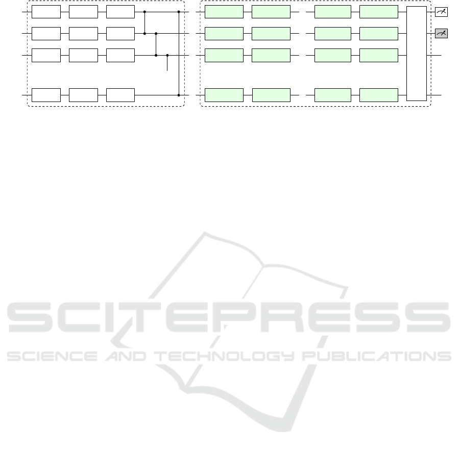
Thus in both quantum and hybrid approaches,
the VQC consists of a horizontally-shifting data re-
uploading VQC, as shown in Figure 2. The VQC has
L layers, each with an angular data embedding block,
a variational block with adjustable parameters θ, and
a CZ circular entanglement block. The first layer has
no data encoding part. The VQC output state is ob-
served using Pauli-Z measurements. In the case of
the main and target actor, the expectation values of
the first two qubits are measured, and then rescaled
using two classical trainable weights. In the case of
the critics, only the first qubit is measured and then
rescaled with one classical variational parameter. In
order to evaluate the scalability of the VQC, ansatzes
of 4 and 8 qubits are used, with 3 and 5 layers.
The main difference between the quantum and the
hybrid approaches is the data pre-processing. In the
case of the quantum approach, only the VQC is used
as function approximator, whereas in the hybrid ap-
proach, a 6 × 6 NN precedes the processing of the
state features by the VQC. The motivation behind
this approach is to enable the agent to harness both
quantum and classical computing in the hybrid case.
Moreover, this would better show a clear contribution
of the quantum module in HQC approaches.
In Table 1 the different weight counts for the
quantum, hybrid, and classical solutions are detailed,
where the total number of weights is W = W
actor
+
W
critic
, where W
actor
= W
ActorNN
+ 3 × q + 3 × l × q +
f × l × q + 2 and W
critic
= W
CriticNN
+ 3 × q + 3 × l ×
q + f × l × q + 2, where q is the qubit count, l is the
number of layers and f is the size of the input. In the
quantum case, W
ActorNN
= W
CriticNN
= 0, while in the
hybrid case W
ActorNN
= 42 and W
CriticNN
= 72, due to
their preprocessing NNs. The actor has f = 6 input
features – the environment state dimension, and the
critic has f = 8 input features, adding the two actions.
5 RESULTS
In this section we analyze the training and testing per-
formance of the HQC DDPG algorithm on the robot
navigation task. We firstly show our main contri-
bution, the ability of this method to tackle a CAS
industrially-relevant use case. Then we look into
the scalability of all DDPG variants presented in this
work: quantum, hybrid, and classical. Furthermore,
we evaluate whether pre-processing the state features
with a 6 × 6 NN brings a computational advantage.
The classical DDPG algorithm employs NNs as
actors and critics. These NNs each have two hid-
den layers, and the number of neurons per hidden
layer was chosen such as to result into a similar
QAIO 2025 - Workshop on Quantum Artificial Intelligence and Optimization 2025
810

Layer 1: U
var
1
Layer L: U
L
. . . . . .
. . . . . .
. . . . . .
.
.
.
.
.
.
. . . . . .
|0⟩
R
X
(θ
(1)
11
) R
Y
(θ
(1)
12
) R
Z
(θ
(1)
13
) R
X
(λ
(L)
11
f
1
)) R
Y
(λ
(L)
12
f
2
)) R
X
(λ
(L)
15
f
5
) R
Y
(λ
(L)
16
f
6
))
U
var
L
o
1
|0⟩
R
X
(θ
(1)
21
) R
Y
(θ
(1)
22
) R
Z
(θ
(1)
23
) R
X
(λ
(L)
21
f
2
)) R
Y
(λ
(L)
22
f
3
)) R
X
(λ
(L)
25
f
6
) R
Y
(λ
(L)
26
f
1
))
o
2
|0⟩
R
X
(θ
(1)
31
) R
Y
(θ
(1)
32
) R
Z
(θ
(1)
33
) R
X
(λ
(L)
31
f
3
)) R
Y
(λ
(L)
32
f
4
)) R
X
(λ
(L)
35
f
1
) R
Y
(λ
(L)
36
f
2
))
|0⟩
R
X
(θ
(1)
n1
) R
Y
(θ
(1)
n2
) R
Z
(θ
(1)
n3
) R
X
(λ
(L)
n1
f
a
)) R
Y
(λ
(L)
n2
f
b
)) R
X
(λ
(L)
n5
f
e
)
R
Y
(λ
(L)
n6
f
f
))
Figure 2: The actor and critic VQC architectures. Here θ
(L)
qg
are the trainable parameters of layer L at qubit q for the g-th gate,
and each classical feature is variationally pre-scaled using λ
(L)
qg
. The classical features are rotationally permutated: the last
layer shows features in order a,b,.. ., f , which is a permutation of {1, 2,. . ., 6}, where a = n mod 6 and n is the qubit count.
In the case of the actor VQC, the first 2 qubits are measured and for the critic VQC, the measurement is done on the first qubit.
weight count between the quantum, hybrid, and clas-
sical solutions. This lead to the 7 × 7, 10 × 10,
12 × 12, and 16 × 16 NN sizes, corresponding to the
c
7,7
, c
10,10
, c
12,12
, and c
16,16
architectures. For a fair
benchmarking, we also look into a bigger classical
DDPG agent, where the actor and the critic each have
a 256 × 256 NN, further referred to as c
256,256
. The
two hidden layers of the NNs use the ReLU activa-
tion function. The output layer of the actor employs
the tanh activation to constrain the action output be-
tween [-1, 1], which is then rescaled between [0, 10]
– the left and right wheel velocities range – using
environment-specific bias and scaling factor. The out-
put layer of the critic uses a linear activation function
to produce the scalar Q-value.
In the case of the quantum approach, the actor and
the critic target and main NNs are replaced by the
horizontally-shifting data re-uploading ansatz of Fig-
ure 2. We applied VQCs of 4 and 8 qubits, each with
3 or 5 layers. For the actor module, that outputs an
action, we observe the first two qubits using Pauli-Z
measurements, and then rescale them using two train-
able weights. For the critic, we measure only the first
qubit and then also rescale it using a trainable weight.
The hybrid solution is similar to the quantum one,
with the difference that the input features are initially
pre-processed with a 6 ×6 NN. Each architecture was
trained in three experiments of 120 000 time steps.
All resulting models were tested on 10 environment
runs. The following subsections will discuss the per-
formance of the models observed during training time
and, respectively, during test time.
5.1 Training Performance
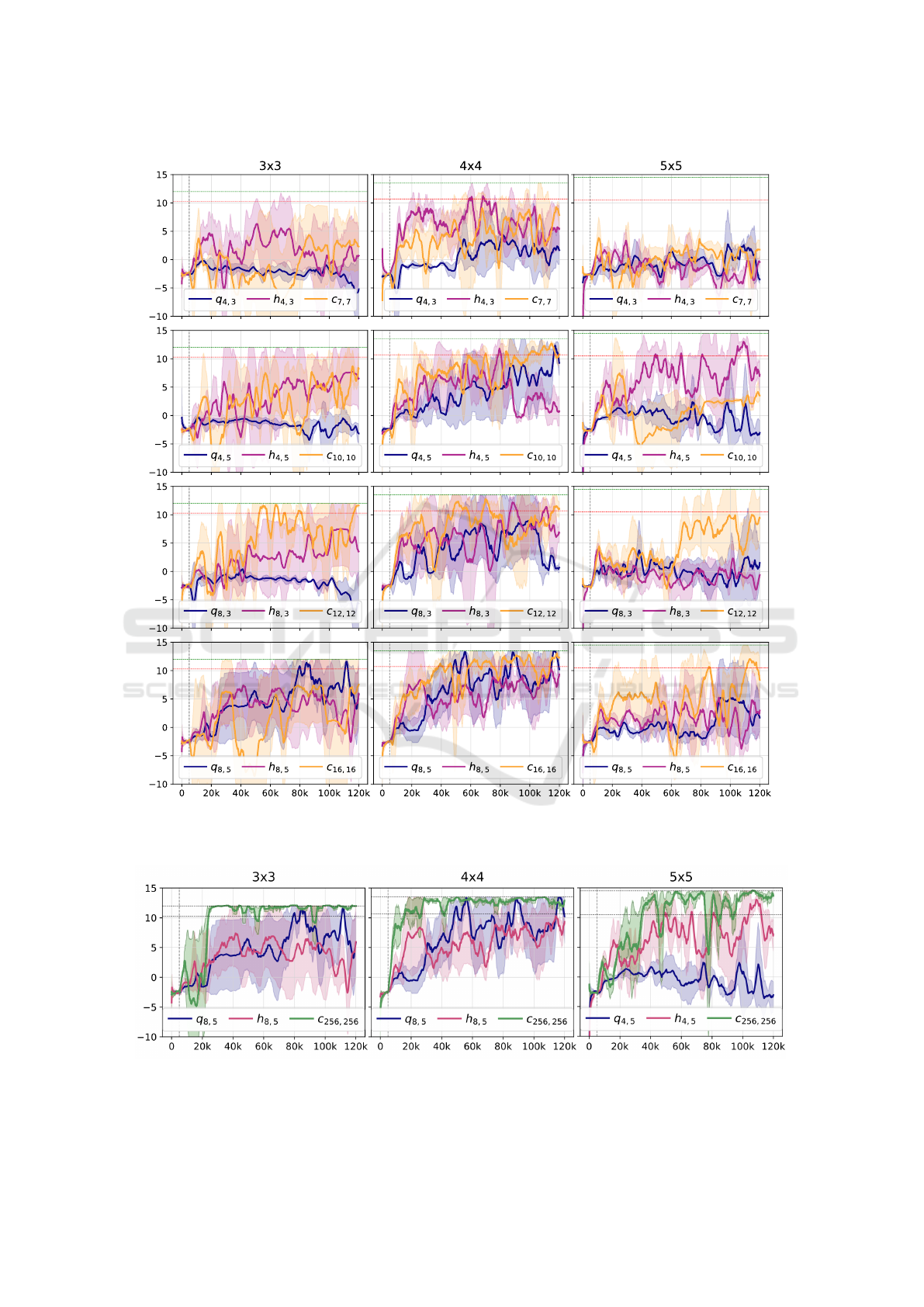
Figures 3 and 4 show that the quantum DDPG we
chose can solve this CAS robot navigation task. De-
spite a weight count of around 3 orders of magnitude
less, the quantum approach of 8 qubits and 5 lay-
ers reaches the t
1
threshold in the 3 × 3 and 4 × 4
mazes, and the hybrid solution with 4 qubits and 5
layers reaches the t
2
threshold in the 5 × 5 environ-
ment. These results also hint towards the need to in-
vestigate the best ansatz for a given task: e.g., despite
the higher complexity of the 5 × 5 map, the smaller
4-qubit hybrid VQC obtained the best results.
When it comes to the scalability of the solutions,
the learning process of quantum architectures is either
improved (q
4,5
and q
8,5
) or unaffected (q
4,3
and q
8,3
)
by adding more qubits. In the case of hybrid archi-
tectures, adding more qubits can even lead to poorer
results (h
4,5
and h
8,5
). Increasing the number of lay-
ers improves quantum results and sometimes pushes
them to reach past the thresholds, but it seems to usu-
ally not impact the training process of hybrid models.
Across all maze dimensions, the hybrid learning
curve is steadier, stabler and reaches higher rewards
than the quantum one, with exceptions: the q
8,5
model
reaches thresholds more often than h
8,5
. Thus, having
a 6 × 6 pre-processing NN, trained together with the
VQC likely leads to more stability and better results.
Quantum-enhanced approaches show similar re-
sults to their classical counterparts. While in half
of the subplots in Figure 3 the classical models learn
faster or reach higher rewards than the HQC models,
for the 3 × 3 map, h
4,3
surpasses c
7,7
, q
8,5
is better
than c
16,16
in the 4 ×4 map, and h
4,5
is more suitable
than c
10,10
in the 5 ×5 map. Thus, the comparison of
similarly-sized models shows that the suitability of a
classical or HQC model depends on both model size
and map configuration.
5.2 Test Performance
In Table 1 the test results of the quantum, hybrid and
classical configurations are displayed. The best re-
ward is obtained by the quantum (q
8,5
) and hybrid
(h
4,5
) methods. Their success rates (SR) and step
Continuous Quantum Reinforcement Learning for Robot Navigation
811

Time Steps
Reward
Figure 3: Training plots of all quantum, hybrid, and classical solutions of similar sizes. Rows present the quantum and hybrid
solutions of 4 and 8 qubits, each with 3 or 5 layers. The green and red horizontal lines correspond to thresholds t
1
and t
2
.
Figure 4: Training curves of the best hybrid and quantum models on all maps, compared to the best performing classical
solution with 256 × 256 NN function approximators. The higher and lower dashed horizontal lines are thresholds t
1
and t
2
.
QAIO 2025 - Workshop on Quantum Artificial Intelligence and Optimization 2025
812

counts are similar to the ones of the best 256 × 256-
NN agent: e.g., the quantum model q
8,5
has a perfect
SR on the 3 × 3 and 4 × 4 mazes. Therefore, also at
test time, the HQC DDPG is shown to be performant
on solving this CAS robot navigation use case.
Considering the increase in SR and in reward, in-
creasing the number of data re-uploading layers from
3 to 5 seems to correlate with a better performance
for the quantum solutions. In the case of the hybrid
solutions, while more layers seems to correlate with
a higher SR, the obtained rewards can even decrease.
E.g., between the h
8,3
and the h
8,5
models, the mean
reward decreases by 16%. Benchmarking on the 5×5
environment leads to inconclusive observations on the
performance metrics: increasing the number of layers
resulted mostly in a decrease of reward and success
rate. The number of steps provides no clear corre-
lation with any architectural size - a wider or deeper
ansatz could both improve or worsen the step count,
as it happens when increasing the layer count on the
8-qubit architecture in the 4 × 4 environment. Thus,
also at test time results point towards a use case de-
pendency of the best approach, with scalability not
guaranteed. This holds also for classical solutions:
more weights do not always lead to higher perfor-
mance: c
16,16
has three times more weights that c
7,7
,
yet obtains a lower mean reward.
We also look into whether the hybrid solutions
perform better than their classical counterparts, that
is, whether the 6 × 6 pre-processing NN improves re-
sults. Test performance metrics show that the hybrid
architectures lead to better overall SR, reward and
step counts on both 3 × 3 and 5 × 5 environments.
A clear exception here is the q
8,5
architecture, which
scores better than h
8,5
on 8 out of 9 benchmarks. On
the 4 × 4 environment, no clear trend emerges - for
the 3-layered VQC, the hybrid approach reaches bet-
ter rewards, while for the 5-layered VQCs, it is the
quantum solution that is superior.
Finally, we investigate whether quantum and hy-
brid approaches could be more desirable for this ap-
plication than the classical ones. When comparing so-
lutions of similar weight counts, namely the groups
{q
4,3
,h
4,3
,c
7,7
}, {q
4,5
,h
4,5
,c
10,10
}, {q
8,3
,h
8,3
,c
12,12
}
and {q
8,5
,h
8,5
,c
16,16
}, one sees different results: in
the first group, the quantum and hybrid solutions lead
to a higher successful run rate and mean reward on the
4 × 4 and 5 × 5 environments, but were less effective
on the 3 × 3 maze. In the last group, the quantum and
hybrid models were better than their classical coun-
terparts of similar size on most benchmarks.
6 CONCLUSION
In this paper, we propose using a quantum-enhanced
deep deterministic policy gradient algorithm in order
to enable a robot to navigate a maze-like environment
using local LIDAR information and feedback incor-
porating relative proximity to goal. We benchmarked
three choices for both the actor and critic of the DDPG
algorithm: classical neural networks, pure variational
quantum circuits with a few classical weights for out-
put scaling, and a hybrid solution where the classi-
cal observation features are pre-processed by a small
6 × 6 neural network. We integrated a data encoding
strategy in the data-reuploading circuit, in which the
order of the classical data features embedded on each
qubit is horizontally cyclically shifted. Each model
was benchmarked on three maze-like environments
of different sizes, number of obstacles and path to
be learnt. The quantum and hybrid models included
ansatzes of 4 and 8 qubits and, respectively, 3 and 5
data re-uploading layers. Five classical models were
tested as comparative benchmarks, with both equiv-
alent numbers of weights, as well as state-of-the-art
number of weights. Each configuration was trained
three times and then tested on 10 environmental runs.
We analysed the training curves and three perfor-
mance metrics: the number of successful runs, the
mean reward, and the number of steps, all measured at
test time. Results show that quantum-enhanced solu-
tions are successful at solving this continuous control
robot navigation task. Quantum and hybrid models
are fairly scalable, but there are exceptions just like in
the classical case, and thus the optimal dimensions of
a quantum ansatz are application-dependent. More-
over, while the high-dimensional classical DDPG ob-
tained higher performance metrics, we identified an
8-qubit ansatz of 3 and 5 layers that behaves compa-
rably with 200 times fewer trainable parameters.
One caveat of the quantum-enhanced solutions,
that we propose as future work, is the fact that they
need more steps than their classical variants in order
to reach the goal at test time. This could be mitigated
either by trying more complex models, or by adapt-
ing the reward function to further guide the robot to
avoid making unnecessary moves. Another poten-
tial building block of this solution is its deployment
on quantum hardware, in order to benchmark how
quantum-enhanced DDPG is affected by noise and
hardware limitations. Nevertheless, for this to hap-
pen, more accessible and performant quantum tech-
nology is needed, since VQC-based QRL assumes
numerous training iterations and quantum-classical
hardware communication overhead. It would also be
relevant to scale up this approach to wider and deeper
Continuous Quantum Reinforcement Learning for Robot Navigation
813

Table 1: Performance comparison of quantum (q), hybrid (h), and classical (c) architectures. Each configuration was tested
using seeds {1, 2, 3} and ten runs per seed, totaling 30 runs per model. The table includes the model identifier, total weights
(θ), and the mean and standard deviation of successful runs (SR) out of 30 (SR/30), rewards and time steps (time steps
calculated from SR only). Models without successful runs display nan for time steps, and best metrics are highlighted in bold.
SR/30 Reward Steps (SR-based)
Model θ 3 × 3 4 × 4 5 × 5 3 × 3 4 × 4 5 × 5 3 × 3 4 × 4 5 × 5
q
4,3
267 0 2 13 −0.53 ± 0.38 1.49 ± 3.35 6.50 ± 7.10 nan 30.00 ± 0.01 60.62 ± 2.63
q
4,5
427 0 30 6 −0.05 ± 0.63 13.50 ± 0.06 4.56 ± 5.16 nan 35.93 ± 3.89 56.00 ± 2.00
q
8,3
531 8 20 10 2.64 ± 5.21 8.79 ± 6.71 5.68 ± 6.31 26.75 ± 1.39 36.95 ± 3.05 57.10 ± 0.99
q
8,5
851 30 30 10 12.11 ± 0.06 13.31 ± 0.22 4.97 ± 7.61 21.37 ± 1.25 33.10 ± 3.49 52.00 ± 0.01
h
4,3
381 18 21 18 7.16 ± 5.60 9.31 ± 6.18 9.52 ± 6.33 25.17 ± 2.55 33.10 ± 3.11 56.72 ± 1.84
h
4,5
541 20 20 28 6.35 ± 7.84 8.15 ± 6.05 13.12 ± 2.97 23.95 ± 1.05 40.75 ± 5.46 51.71 ± 5.56
h
8,3
645 22 20 1 8.70 ± 4.99 8.96 ± 6.24 1.75 ± 2.70 27.41 ± 1.44 35.55 ± 0.60 48.00 ± nan
h
8,5
965 20 28 14 7.27 ± 5.48 11.77 ± 3.85 4.65 ± 7.19 26.60 ± 2.84 40.61 ± 1.75 60.64 ± 7.96
c
7,7
248 20 20 10 8.22 ± 5.57 8.44 ± 7.26 5.85 ± 6.65 19.00 ± 0.01 31.40 ± 0.94 46.20 ± 4.89
c
10,10
413 14 24 14 5.55 ± 6.17 7.67 ± 11.01 6.85 ± 6.03 19.71 ± 0.61 37.00 ± 10.09 55.00 ± 6.41
c
12,12
543 25 26 20 9.84 ± 4.24 11.28 ± 4.43 10.03 ± 6.69 20.56 ± 1.45 30.58 ± 2.25 43.35 ± 4.65
c
16,16
851 20 20 26 7.60 ± 6.48 9.24 ± 6.11 11.99 ± 5.87 20.05 ± 1.10 29.50 ± 0.51 49.54 ± 1.73
c
256,256
136 451 30 30 30 12.12 ± 0.09 13.31 ± 0.27 14.81 ± 0.24 18.13 ± 1.70 30.93 ± 2.24 42.93 ± 2.38
ansatzes, to better observe the scalability and poten-
tially the advantage of more complex QRL models.
REFERENCES
Acuto, A. et al. (2022). Variational quantum soft actor-critic
for robotic arm control.
Akbar, M. A., Khan, A. A., and Hyrynsalmi, S. (2024).
Role of quantum computing in shaping the future of
6g technology. Information and Software Technology,
170:107454.
Alagic, G. et al. (2016). Computational security of quan-
tum encryption. In Nascimento, A. C. and Barreto, P.,
editors, Information Theoretic Security, pages 47–71,
Cham. Springer International Publishing.
Bauer, B. et al. (2020). Quantum algorithms for quantum
chemistry and quantum materials science. Chemical
Reviews, 120(22):12685–12717.
Brockman, G. et al. (2016). Openai gym. arXiv preprint
arXiv:1606.01540.
Caro, M. C. et al. (2022). Generalization in quantum ma-
chine learning from few training data. Nature Com-
munications, 13(1).
Chen, S. Y.-C. (2023). Asynchronous training of quantum
reinforcement learning. Procedia Computer Science,
222:321–330. International Neural Network Society
Workshop on Deep Learning Innovations and Appli-
cations (INNS DLIA 2023).
Dalzell, A. M. et al. (2023). Quantum algorithms: A survey
of applications and end-to-end complexities.
Dr
˘
agan, T.-A. et al. (2022). Quantum reinforcement learn-
ing for solving a stochastic frozen lake environment
and the impact of quantum architecture choices.
Hohenfeld, H. et al. (2024). Quantum deep reinforcement
learning for robot navigation tasks. IEEE Access,
12:87217–87236.
Huang, S., Dossa, R. F. J., Ye, C., and Braga, J. (2021).
Cleanrl: High-quality single-file implementations of
deep reinforcement learning algorithms.
Kruse, G. et al. (2024). Variational quantum circuit design
for quantum reinforcement learning on continuous en-
vironments. In Proceedings of the 16th International
Conference on Agents and Artificial Intelligence, page
393–400.
K
¨
olle, M. et al. (2024). Quantum advantage actor-critic for
reinforcement learning.
Lan, Q. (2021). Variational quantum soft actor-critic.
Lillicrap, T. P. et al. (2019). Continuous control with deep
reinforcement learning.
McArdle, S. et al. (2020). Quantum computational chem-
istry. Reviews of Modern Physics, 92(1):015003.
Meyer, N. et al. (2024). A survey on quantum reinforcement
learning.
Mnih, V. et al. (2015). Human-level control through deep
reinforcement learning. nature, 518(7540):529–533.
Moll, M. and Kunczik, L. (2021). Comparing quantum
hybrid reinforcement learning to classical methods.
Human-Intelligent Systems Integration, 3(1):15–23.
Periyasamy, M. et al. (2024). Bcqq: Batch-constraint quan-
tum q-learning with cyclic data re-uploading. In 2024
International Joint Conference on Neural Networks
(IJCNN), pages 1–9. IEEE.
Senokosov, A. et al. (2024). Quantum machine learning for
image classification. Machine Learning: Science and
Technology, 5(1):015040.
Skolik, A., Jerbi, S., and Dunjko, V. (2022). Quantum
agents in the gym: a variational quantum algorithm
for deep q-learning. Quantum, 6:720.
Wu, S. et al. (2023). Quantum reinforcement learning in
continuous action space.
Yang, Z., Zolanvari, M., and Jain, R. (2023). A survey of
important issues in quantum computing and commu-
nications. IEEE Communications Surveys & Tutori-
als, 25(2):1059–1094.
QAIO 2025 - Workshop on Quantum Artificial Intelligence and Optimization 2025
814