A Framework for Identifying Underspecification in Image Classification
Pipeline Using Post-Hoc Analyzer
Prabhat Parajuli and Teeradaj Racharak
∗ a
School of Information Science, Japan Advanced Institute of Science and Technology, Japan
Keywords:
Underspecification Detection, Explainable AI, Spurious Correlation, Rashomon Effect, Feature Selection.
Abstract:
Underspecification — a failure mode where multiple models perform well during development but fail to gen-
eralize to new, unseen data due to reliance on insufficient or spurious features — remains critical challenge
in machine learning (ML) and deep learning (DL). In this paper, we focus on a specific aspect of underspec-
ification: the inconsistency in feature learning. We hypothesize that models with similar performance should
exhibit consistent behavior in terms of feature reliance. However, in practice — especially in deep learning —
this consistency is often lacking due to various factors influencing the learning process. To uncover where this
inconsistency occurs, we propose a framework leveraging XAI techniques (specifically LIME and SHAP) to
identify underspecification by analyzing inconsistencies across ML pipeline components, including feature ex-
tractors, optimizers, and weight initialization. Experiments on MNIST, Imagenette, and Cats vs Dogs reveal
significant variability in feature reliance, particularly due to the choice of feature extractor. This variability
highlights how different factors contribute to the learning of varied features, ultimately leading to potential
underspecification. While this study focuses on the impact of specific pipeline components, our framework
can be extended to analyze other factors contributing to underspecification in machine learning systems.
1 INTRODUCTION
Despite the remarkable advancements of Machine
learning (ML) and Deep Learning (DL) algorithms,
concerns about their reliability, interpretability, and
trustworthiness remain significant (Kamath and Liu,
2021; Li et al., 2023; Molnar, 2020). One signifi-
cant threat undermining these crucial properties from
the modeling pipeline of ML is underspecification —
where the modeling pipelines perform strongly well
in the development settings but fail to generalize to
the real-world settings. It is well studied that factors
such as the limitations of empirical risk minimization
(ERM), which prioritize error minimization over ro-
bust feature learning (Teney et al., 2022), along with
distribution shifts (Ovadia et al., 2019; Qui
˜
nonero-
Candela et al., 2022), inadequate data quality and rep-
resentation (D’Amour et al., 2022; Hinns et al., 2021),
and model complexity, can often exacerbate this prob-
lem. From the literature, underspecification oc-
curs when the modeling pipeline — ranging from
data curation to learning algorithms — fails to suf-
ficiently constrain the predictor for a target prob-
a
https://orcid.org/0000-0002-8823-2361
∗
Corresponding author.
lem, leading to multiple valid but divergent solu-
tions.
Roughly, this issue can be viewed from two per-
spectives. First, from the predictive perspective, an
ML pipeline is considered underspecified if it can
yield multiple plausible outcomes for the same in-
put, indicating ambiguity in its predictions (Madras
et al., 2019). That is, the model has not learned
a definitive way to represent the input. Second,
from the training perspective, insufficient specificity
across various components of the pipeline — in-
cluding data preprocessing (Bouthillier et al., 2021),
model architecture, weight initialization (Alahmari
et al., 2020; D’Amour et al., 2022), hyperparame-
ter settings (Arnold et al., 2024; Bischl et al., 2023;
M
¨
uller et al., 2023), and others — can lead the
model to learn different, potentially inconsistent be-
haviors during training. These inconsistencies arise
because the model’s inherent inductive biases, shaped
by the pipeline’s design choices, can influence how
the model prioritizes features during learning. As a
result, the model may emphasize different features,
some of which may be irrelevant, leading to divergent
learned representations (Mehrer et al., 2020). In this
paper, we particularly focus on the later perspective.
426
Parajuli, P. and Racharak, T.
A Framework for Identifying Underspecification in Image Classification Pipeline Using Post-Hoc Analyzer.
DOI: 10.5220/0013374200003905
Paper published under CC license (CC BY-NC-ND 4.0)
In Proceedings of the 14th International Conference on Pattern Recognition Applications and Methods (ICPRAM 2025), pages 426-436
ISBN: 978-989-758-730-6; ISSN: 2184-4313
Proceedings Copyright © 2025 by SCITEPRESS – Science and Technology Publications, Lda.

(a) Selected Test image (b) LIME explanations (c) SHAP explanations
Figure 1: An example of underspecification in model explanations for an “English Springer” input from the Imagenette
testset. DenseNet121 models trained with identical pipelines but different random seeds yield varying feature-importance
explanations. (a) An image of interest. (b) LIME explanations for seeds 0, 1, and 6, highlighting positive features. (c) SHAP
explanations for the same models; red is positive, and blue is negative. These variations highlight initialization effects.
This phenomenon is closely analogous to the well-
known “Rashomon Effect” (Breiman, 2001), where
models with varying structures (called the Rashomon
set) can fit with the training data equally well but rely
on different features. In deep learning, such effects
are amplified by the aforementioned design choices
made during training, which collectively shape the
model’s learning trajectory. Thus, models with dif-
ferent architectures may achieve similar performance
on the same dataset yet rely on entirely or partially
distinct features. While some models may capture
robust, generalizable patterns, others might exploit
noise or spurious correlations, raising concerns about
their reliability on unseen data.
Under ideal conditions — where the pipeline
components influencing the learning process (e.g.,
data quality, optimization methods, model complex-
ity, etc.) are properly controlled — it is reasonable
to expect that any well-specified pipeline will exhibit
more consistent behavior and rely on similar feature
representations across models. However, even in such
conditions, subtle differences in optimization dynam-
ics or model architecture can introduce some vari-
ability. In underspecified systems, this variability is
amplified, causing models that perform well during
development to rely on differing feature representa-
tions, leading to significant differences in behavior
during deployment, highlighting the issue of under-
specification. Figure 1 illustrates this phenomenon —
varying only the initial weights with different random
seeds (see Subsection 4.1) while keeping all other
pipeline components identical reveals, through LIME
and SHAP explanations, that random initializations
influence the model’s feature learning mechanisms.
In this paper, we aim to identify underspecifica-
tion within ML pipelines by pinpointing the compo-
nents that contribute most to divergent learning pro-
cesses. We propose a framework using posthoc anal-
ysis techniques, namely Local Interpretable Model-
Agnostic Explanations (LIME) (Ribeiro et al., 2016)
and SHapley Additive exPlanation (SHAP) (Lund-
berg and Lee, 2017), to analyze variations in feature-
learning behavior. Our framework posits that mod-
els with similar development performance should ex-
hibit consistent feature reliance, and any variability
in explanation features signals a certain degree of un-
derspecification. We validate this framework through
experiments on MNIST (LeCun et al., 1998), Ima-
genette (Howard, 2019), and Cats vs Dogs (Kaggle,
2013) datasets. Our findings indicate that feature ex-
tractor architecture plays a more significant role in un-
derspecification than other pipeline components.
2 RELATED WORKS
Underspecification in machine learning (ML) occurs
when models perform well on in-distribution data but
fail to generalize to out-of-distribution (OOD) or un-
seen data. A study (D’Amour et al., 2022) revealed
that models trained with different random initializa-
tions can exhibit significant variations in their OOD
performance despite similar in-distribution accuracy,
underscoring that high development accuracy does
not necessarily indicate a reliable model, especially
in complex or dynamic environments.
Ensemble methods, for example, have been used
to quantify uncertainties, distinguishing between
epistemic and aleatoric types (Lakshminarayanan
et al., 2017; Ovadia et al., 2019). These stud-
ies demonstrate that underspecification contributes to
epistemic uncertainty — uncertainty due to model pa-
rameters — which can be undermine model reliabil-
ity, particularly in high-stakes applications where pre-
dictability is key. Moreover, several works have fo-
cused on OOD generalization, proposing techniques
like domain adaptation (Teney et al., 2022) and eval-
uating models on local geometric loss properties
(Madras et al., 2019). These methods aim to identify
and mitigate performance degradation when models
are exposed to new, unseen distributions. Addition-
A Framework for Identifying Underspecification in Image Classification Pipeline Using Post-Hoc Analyzer
427

ally, (Hinns et al., 2021) explored the role of dataset
quality and representativeness in underspecification,
highlighting how the training data itself introduce bi-
ases and inconsistencies that affect model robustness.
While these studies offer valuable insights into
various aspects of underspecification, they generally
do not investigate “how specific components of the
ML pipeline, contribute to the variability in feature
reliance and decision-making”. Early-stage pipeline
choices have significant implications for model be-
havior but remain underexplored in the context of un-
derspecification.
In contrast, our study systematically measures
variability in feature learning across different ML
pipeline configurations. By varying pipeline compo-
nents and using post-hoc tools like LIME and SHAP,
we quantify their impact on model decision-making.
This work advances understanding of underspecifica-
tion by identifying key contributing components and
emphasizing the need for more interpretable models.
3 PROPOSED FRAMEWORK
Our framework is designed to quantify the degree of
underspecification in the context of supervised learn-
ing settings by allowing practitioners to systemati-
cally vary individual components of their machine
learning pipeline. We also demonstrate their appli-
cations on the image classification task. We formalize
the pipeline as an n-tuple representation and describe
a generalized approach to measure the impact of vary-
ing any single component on the underspecification
1
.
3.1 Pipeline Representation
Any machine learning pipeline P
i
can be represented
as a n-tuple P
i
:
= (p
1
, p
2
, . . . , p
n
), where n ∈ Z
+
and
each p denotes a distinct component of the pipeline,
such as, data preprocessing, feature extraction, clas-
sifiers, or optimization methods. In our framework,
the index i is used to enumerate multiple pipelines
by varying specific components, enabling controlled
comparisons across different configurations. When it
is clear from the context, i might be omitted.
Our objective is to analyze the degree of under-
specification by varying individual components p
j
of
the pipeline P while fixing other components, en-
abling to study the effect of a specific component of
the learned representations and predictive behavior of
the ML pipeline.
1
Our implementation source code is available online
at: https://github.com/realearn-jaist/underspecification-in-
computer-vision
3.2 Framework Overview
Our framework is composed of the following steps:
3.2.1 Component Selection and Variation
We select a specific component p
j
of the ML pipeline
for underspecification analysis. For instance, it could
be the feature extractor, optimizer, etc. For any se-
lected p
j
, a finite set of k-variations {p
k
j
| k ∈ Z
+
, 1 ≤
k ≤ m} is computed, where m represents the total
number of variations considered. This choice of p
j
generates a set of ML pipelines {P
i
| 1 ≤ i ≤ k} to test
the underspecification, where each pipeline P
i
is con-
structed as P
i
:
= (p
1
, . . . , p
i
j
, . . . , p
n
), differing solely
in the specified component p
j
. For instance, if we
choose to vary the feature extractor component p
j
,
the variations might correspond to different network
architectures, e.g., CNN, ResNet, or VGG.
3.2.2 Pipeline Modeling and Training
Next, each pipeline P
i
is complete by attaching with a
predictor (or classifier) g
i
for training with a training
set D
tr
, drawn from a dataset D; we divide D into sub-
sets of training (D
tr
), validation (D
val
), and test (D
test
)
while reserving D
test
for later use, i.e., generating ex-
planations and analyzing underspecification.
In our procedure, any completed pipeline P
i
takes
in D
train
to produce a function m
i
, which maps from
any input x into label y. Explicitly, each pipeline P
i
can be thought of as a composite function m
i
(x)
:
=
g
i
( f
i
(x)), where f
i
and g
i
represent a feature extrac-
tor and classifier, respectively. Thus, we use the term
“model” from now onward, which essentially repre-
sents an individual pipeline. To illustrate this process,
Algorithm 1 provides the procedure to generate a set
M of models by varying specific component p
j
across
its predefined values. It takes as input the dataset D
and the variation set P
j
, iteratively creates a set P
i
of
pipeline candidates with each variation p
j
∈ P
j
, and
stores the trained models m
i
in the set M. This set of
models is then used in subsequent steps for explana-
tion generation and underspecification measurement.
Furthermore, in order to ascertain that any inter-
pretability differences observed across the models are
not attributed to performance disparities, we ensure
that each model achieves a predefined performance
threshold t on both D
val
and D
test
.
3.2.3 Explanation Generation and
Underspecification Measurement
For each test sample x ∈ D
test
and model m
i
given
by a pipeline P
i
, the next step is to generate expla-
ICPRAM 2025 - 14th International Conference on Pattern Recognition Applications and Methods
428

Algorithm 1: Model Generation with Pipeline Variations.
Input : dataset: D, set of variations for a
chosen component p
j
: P
j
,
predefined threshold: t
Output: Set of trained models: M
1 Function
train and validate(P
i
, D
tr
, D
val
, D
test
):
2 train(m
i
, D
tr
);
3 if eval(m
i
, D
val
) ≥ t and
eval(m
i
, D
test
) ≥ t then
4 return m
i
;
5 return None;
6 Function create models(D, P
j
):
7 split(D, D
tr
, D
val
, D
test
);
8 M ← [];
9 foreach v ∈ P
j
do
10 P
i
← construct pipeline(. . . , v, . . . );
11 m
i
←
train and validate(P
i
, D
tr
, D
val
, D
test
);
12 if m
i
̸= None then
13 M.append(m
i
);
14 return M;
nations ξ
m
i
x
using LIME and SHAP. These explana-
tions highlight the features reliance that contribute
to the model’s predictions, allowing for a compari-
son of predictive behavior across models given by the
pipelines. Consequently, we quantify the degree of
underspecification by measuring the variation in ex-
planations across models:
UnderspecificationDegree
:
= Variation

ξ
m
i
(x)
k
i=1

,
where ξ
m
i
x
is the explanation given by model m
i
for
input x, and Variation(·) is a metric such as cosine
distance or any other metric that quantifies differences
between explanations.
Using LIME and SHAP for model-agnostic inter-
pretability, we explore underspecification from both
instance and class perspectives.
3.3 Instance-Level Underspecification
The instance-level underspecification refers to a sit-
uation extended for analyzing any individual in the
dataset. This view is necessary to analyze which in-
stance the ML pipeline fails to generalize. Intuitively,
we compare the explanations between the models in
M and inspect the input x from D
test
assessing the con-
sistency or variability of their local behavior.
Formally, let x be a test instance in D
test
. For any
model m
i
∈ M, the predicted label is y
:
= m
i
(x). To
provide an explanation of the features of x that con-
tribute to this prediction, we apply both LIME and
SHAP independently (one at a time). Let ξ
m
i
x
denote
the explanation generated by the chosen method (ei-
ther LIME or SHAP). We gather explanations from
all models for x as: Ξ
:
= {ξ
m
1
x
, ξ
m
2
x
, . . . , ξ
m
k
x
}
The instance-level comparison can thus be defined
as follows: The cosine similarity metric, which allows
us measure angular differences between explanation
vectors, focuses on orientation rather than magnitude.
Specifically, we compute the pairwise cosine distance
(denoted by d) for all possible pairs of explanations

ξ
m
i
x
, ξ
m
j
x

, where i ̸= j as:
d

ξ
m
i
x
, ξ
m
j
x

:
= 1 −
ξ
m
i
x
· ξ
m
j
x
∥ξ
m
i
x
∥∥ξ
m
j
x
∥
(1)
As the explanations are binarized for the calcula-
tion process (see details in Subsection 4.2), the cosine
distance d

ξ
m
i
x
, ξ
m
j
x

ranges from 0 to 1. A value of
0 indicates perfect similarity (maximum consistency)
between explanations, while a value of 1 represents
no similarity at all (maximum variability).
Figure 2 depicts the general workflow for
instance-level underspecification analysis procedure
at test time, where we vary only weight initialization
with different seeds during training and analyze the
variations in explanations at test time.
3.4 Class-Level Underspecification
The instance-level underspecification gives one per-
spective to quantify this problem in the ML pipeline.
It still does not capture the overall predictive behav-
ior of the model pipeline. To gain more comprehen-
sive understanding and quantify overall behavior, we
select a set of instances associated with class c
i
. Se-
lecting instances can be somewhat subjective, as these
instances should ideally represent the overall class’s
feature distribution. To mitigate this concern, we first
select a diverse set of instances from D
test
that cap-
ture a range of feature variations within the class. We
then filter out incorrectly predicted instances, retain-
ing only those that are correctly predicted by all mod-
els in M. The resulting set X, ensures that the remain-
ing instances reflect the class’s feature distribution
and provide reliable, consistent predictions across all
models. Using LIME or SHAP, each model m
i
can be
provided an explanation ξ
m
i
x
l
for any instance x
l
∈ X.
We then compute ClassLevelScore (denoted by
ˆ
d) by
averaging the instance-level underspecification of ex-
planation pairs (ξ
m
i
x
l
, ξ
m
j
x
l
) across all instances in X:
ˆ
d(m
i
, m
j
)
:
=
1
|X|
|X|
∑
l=1
d(ξ
m
i
x
l
, ξ
m
j
x
l
) (2)
A Framework for Identifying Underspecification in Image Classification Pipeline Using Post-Hoc Analyzer
429

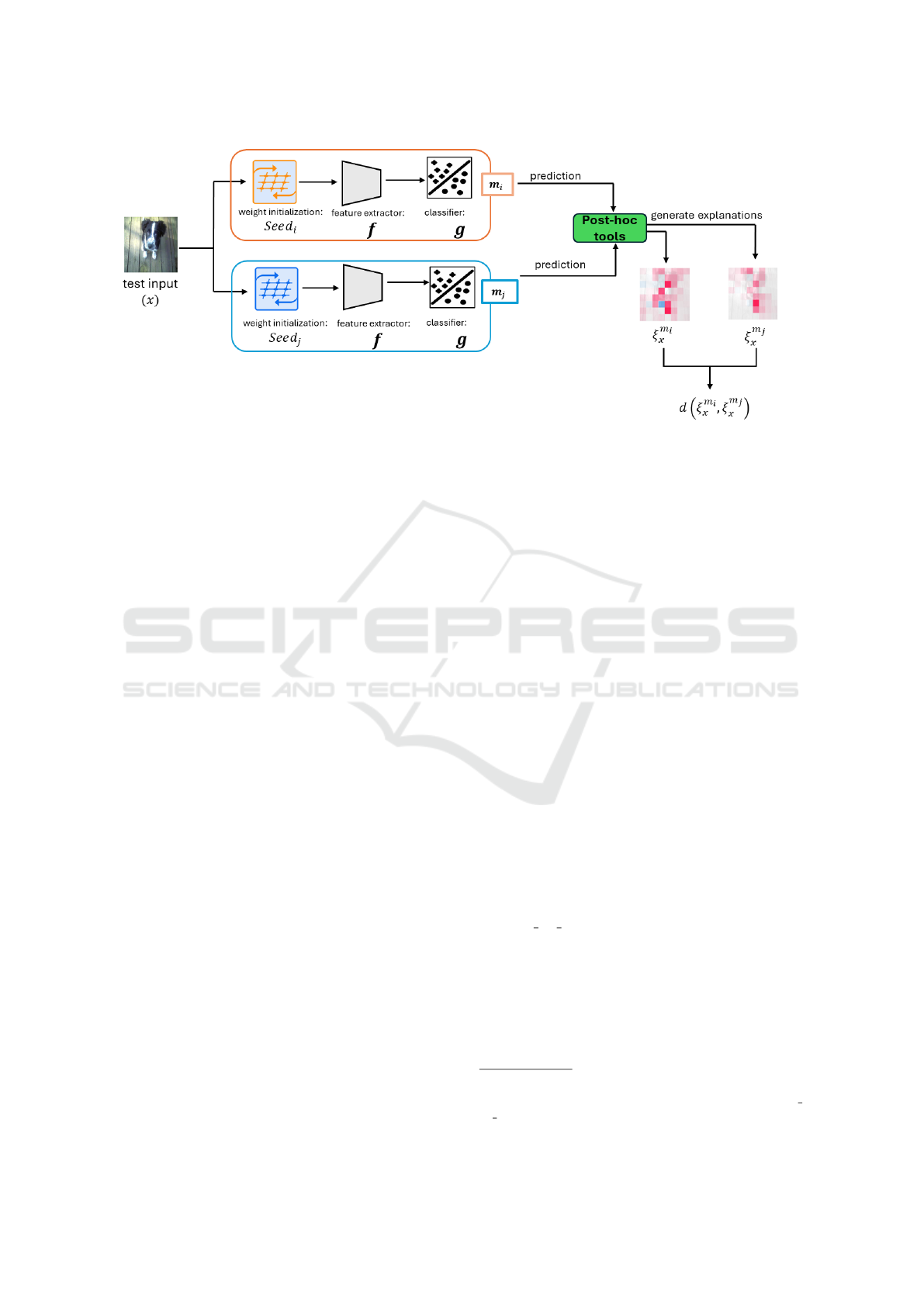
Figure 2: An example workflow for instance-level underspecification analysis at test time. Here, a test input x is drawn
from D
test
, and passed through two models, m
i
: g( f (x))
seed
i
and m
j
: g( f (x))
seed
j
, each shaped by different weight initial-
ization: Seed
i
and Seed
j
, while keeping all other components, such as, D
tr
, feature extractor f , classifier-head g, etc., fixed
during training. Post-hoc explanation tools (e.g., SHAP in this case) are then used to analyze and compare the generated
explanations, revealing the influence of weight initialization on model predictions and their interpretability.
where | · | represents the set cardinality and
ˆ
d ranges
from 0 to 1. The lower
ˆ
d indicate higher consistency
and lower degrees of underspecification for the class
c
i
, while the higher scores imply greater variability
and higher degrees of underspecification.
4 EXPERIMENTS AND ANALYSIS
In this work, we investigate the roles of various com-
ponents within the ML pipeline to identify which
component contributes most to underspecification
problem. To achieve this, we systematically vary spe-
cific components of the ML pipeline while keeping
all other components constant and then analyze the
resulting feature reliance using LIME and SHAP. Our
focus in this work is mainly on three components of
the pipeline — feature extractor, optimizer, and initial
weight — as these are potential sources of variation
in model behavior under underspecified conditions.
4.1 Experimental Setup
The ML pipelines in this study are designed to iso-
late the impact of specific components by changing
one component at a time, enabling us to observe the
relative contribution of each component to variation
in feature reliance, reflecting underspecification prob-
lem. That is, for each experiment (each dataset),
we vary one component at a time across three pri-
mary phases: feature extractors, optimizers, and ini-
tial weights. The remaining components are held con-
stant to ensure any observed differences in feature re-
liance are due to the varied component. The following
pipeline’s configurations are used:
1. Dataset: Each experiment is conducted on three
datasets with different levels of complexity:
MNIST: It is a relatively small, clean dataset of
28 × 28 handwritten digits, ideal for testing the
impact of complex models over simple tasks. We
resize them to 32 ×32 using bilinear interpolation,
making it suitable for implementing different pre-
trained architectures. It includes 60,000 training
images and 10,000 validation images, from which
we create a test set of 2,000 images.
Imagenette
2
: A subset of the ImageNet dataset
with 10 classes that contains large-scale, detailed
backgrounds, introducing additional complexity.
We employ a “320 px” version of it containing
approximately 9,500 training images and about
3,920 validation images, from which we create a
test set by taking 20% of it. Again, the bilinear
interpolation method is used to resize the images
to 224 × 224.
Cats vs. Dogs: It is a binary classification dataset
from a past Kaggle competition, consisting of
detailed images with higher intra-class variation,
offering another layer of complexity. We em-
ploy the dataset from the Tensorflow Dataset
3
li-
brary, where the dataset was preprocessed and
corrupted data were excluded, consisting approx-
imately 25,000 images. Here, the images are re-
2
https://github.com/fastai/imagenette
3
https://www.tensorflow.org/datasets/catalog/Cats\ v
s\ Dogs
ICPRAM 2025 - 14th International Conference on Pattern Recognition Applications and Methods
430

Table 1: Training, validation (Val), and test accuracy (Acc) of models with different feature extractors and optimizers across
datasets.
Dataset Configuration Model Train Acc (%) Val Acc (%) Test Acc (%)
MNIST
Feature Extractor CNN 98.92 99.00 99.35
MobileNet 99.61 98.84 99.20
DenseNet121 99.88 99.25 99.45
EfficientNetB0 98.79 98.33 98.95
Optimizer CNN-Adam 99.57 99.00 99.45
CNN-SGD 98.92 99.00 99.35
CNN-RMSprop 99.60 99.14 99.40
CNN-Nadam 99.55 99.14 99.20
Imagenette
Feature Extractor Xception 99.69 98.45 98.31
InceptionV3 99.43 97.91 97.26
DenseNet121 98.64 98.40 97.79
ResNet50V2 99.25 98.10 97.66
Optimizer DenseNet-Adam 98.92 98.35 98.30
DenseNet-SGD 97.63 98.43 97.27
DenseNet-RMSprop 98.60 98.45 97.79
DenseNet-Nadam 98.91 98.23 97.65
Cats vs Dogs
Feature Extractor Xception 98.88 98.64 98.72
InceptionV3 98.90 98.74 99.22
DenseNet121 98.56 98.08 98.77
ResNet50V2 98.98 98.50 98.44
Optimizer DenseNet-Adam 98.52 97.97 98.83
DenseNet-SGD 97.92 98.11 98.94
DenseNet-RMSprop 98.41 98.71 99.22
DenseNet-Nadam 98.68 98.60 99.16
sized to 224×224 using bilinear interpolation and
created a validation set by splitting 80:20, then re-
serving 20% of the validation set for testing.
2. Varying Feature Extractors: For those pipelines
where we vary the feature extractor component
while keeping all others fixed, we use different ar-
chitectures. The development performances are
summarized in Table 1.
For MNIST: Four different architectures — a
custom CNN and three pretrained architectures:
MobileNet (Howard et al., 2017), DenseNet121
(Huang et al., 2017), and EfficientNetB0 (Tan
and Le, 2019) were tested. Given MNIST’s sim-
plicity, overly complex models would be exces-
sive; thus, these architectures were selected care-
fully to balance model parameters and complex-
ity. For instance, the custom CNN is relatively
shallow, capturing basic spatial hierarchies in the
MNIST digits, while others are deeper networks
typically applied to more complex datasets. Al-
though each architecture differs in its approach
to feature learning, we consider them ideal can-
didates as long as they perform equally well dur-
ing training time. For the pretrained architectures,
we retained only the architectural structure with-
out any pre-initialized weights, i.e., we trained
them from scratch. For training, we found that the
Stochastic Gradient Descent (SGD) optimizer was
effective and smooth across all models. To ensure
a fair comparison, we set the training duration to
15 epochs for each architecture. To prevent over-
fitting, we incorporated dropout layers and L2 reg-
ularization of strength 0.01, especially for deeper
networks like DenseNet121 and EfficientNetB0.
For Imagenette and Cats
vs Dogs: We lever-
aged transfer learning (as both datasets align
with the ImageNet domain) and utilized four pre-
trained architectures — Xception (Chollet, 2017),
DenseNet121 (Huang et al., 2017), InceptionV3
(Szegedy et al., 2016), and ResNet50V2 (He et al.,
2016). These deeper, complex architectures were
chosen for their suitability to larger, more com-
plex datasets compared to MNIST.
For consistency, we applied the same classifier
head structure (g) as in the MNIST experiments.
The Adam optimizer, with its adaptive learning
rate, proved most effective for these architectures,
ensuring smooth convergence. Training over 10
epochs was sufficient to achieve stable perfor-
mance on both datasets.
3. Varying Optimizers: In the second phase of
our experiments, we explored the effects of vary-
A Framework for Identifying Underspecification in Image Classification Pipeline Using Post-Hoc Analyzer
431

ing the optimizer while keeping all other pipeline
components fixed, including the dataset, feature
extractor, classifier structure (deep layers, regular-
izers, etc.), and initialization weights. Upon test-
ing, four optimizers — Adam (Kingma, 2014),
SGD (Ruder, 2016), RMSprop (Hinton, 2012),
and Nadam (Dozat, 2016) — demonstrated simi-
lar performance during training. As for the feature
extractor, we used a simple CNN for MNIST and
DenseNet121 for the other two, chosen for their
relative complexity (least complex in terms of pa-
rameters than others used in the earlier phase).
Training configurations were adapted based on
dataset complexity and optimizer performance.
For instance, on MNIST, all optimizers achieved
similarly high accuracy within 15 epochs, though
some optimizers required additional tuning on the
other two datasets. The development accuracies
are summarized in Table 1.
4. Varying Initial Weights: To investigate the im-
pact of initial weight variations on feature learn-
ing, we introduced different random seeds for ini-
tialization while keeping all other pipeline com-
ponents constant. This setup isolates the ef-
fects of initialization on underspecification. Fol-
lowing a similar configuration as in the “Vary-
ing Optimizers” experiment, we used Adam
as the sole optimizer and applied a CNN for
MNIST and DenseNet121 for both Imagenette
and Cats vs Dogs. Each model was trained ten
times with different random seeds — resulting
in ten CNN and ten DenseNet121 models — to
measure the consistency of feature reliance across
different initializations. Training epochs varied
based on dataset complexity and model conver-
gence’s requirements to achieve comparable ac-
curacy. The development accuracy scores closely
align with the baseline scores from the “Vary-
ing Optimizers” experiment (specifically, the
configurations for CNN-Adam for MNIST and
DenseNet121-Adam for the other two datasets).
Given that the accuracy results for all ten CNN
and ten DenseNet models are similar to these
baselines in Table 1 , we would like to omit them
for clarity and conciseness.
4.2 Underspecification Analysis
Observing the development accuracy scores in Table
1 alone does not clarify whether these scores arise
from reliance on spurious or irrelevant features, which
could indicate an underspecification issue. This ambi-
guity underscores the need for further analysis to un-
derstand feature reliance. To this end, we employed
two widely-used explanation techniques — LIME and
SHAP — to probe the models’ decision-making pro-
cesses. By analyzing which features are most in-
fluential across different configurations of the ML
pipeline, we can assess the extent to which each com-
ponent contributes to variability in feature reliance
and, thereby, to underspecification.
4.2.1 LIME and SHAP Configuration
For LIME, we used the ImageExplainer module with
1,000 perturbed samples per instance, focusing on the
top-3 features for multiclass problems and top-2 for
binary classification. The kernel width was set to 3
for MNIST (with the default slic segmentation) and
left at default for the other two datasets, with output
restricted to positive features for interpretability.
For SHAP, the SHAP Explainer module with the
default partition explainer for image data was used.
Explanations were generated using 1,000 model eval-
uations with the inpaint telea masker technique. To
improve efficiency, we focused only on the top-1 fea-
ture for the probable class.
Both methods assessed the impact of feature ex-
tractor, optimizer, and initial weights on feature re-
liance. To manage computational load, we analyzed
100 instances per MNIST class and 50 per class for
Imagenette and Cats vs Dogs datasets.
To compare feature explanations across configu-
rations, we used the proposed ClassLevelScore metric
(Section 3). Explanations were standardized to binary
masks: for LIME, binary masks of superpixels were
used directly; for SHAP, pixels exceeding 20% of the
maximum positive SHAP value were set to 1, while
the rest were set to 0. These binary representations
facilitated consistent pairwise comparisons using co-
sine distance.
4.2.2 Interpretating Explanations
Our analysis using LIME and SHAP reveals the ex-
tent to which different components of the ML pipeline
contribute to feature reliance underspecification. Our
instance-level underspecification examines the vari-
ability in feature importance explanations for a sin-
gle test instance when specific pipeline components
are varied. Our analysis, conducted on a random test
sample from MNIST D
test
(Figure 3), highlights the
sensitivity of instance-level explanations to changes
in the feature extractor, optimizer, and initial weights.
When varying the “feature extractor,” the expla-
nations and pairwise cosine distance scores in Figure
3 revealed contrasting behaviors between LIME and
SHAP. LIME explanations appeared relatively consis-
tent, whereas SHAP explanations exhibited the high-
ICPRAM 2025 - 14th International Conference on Pattern Recognition Applications and Methods
432

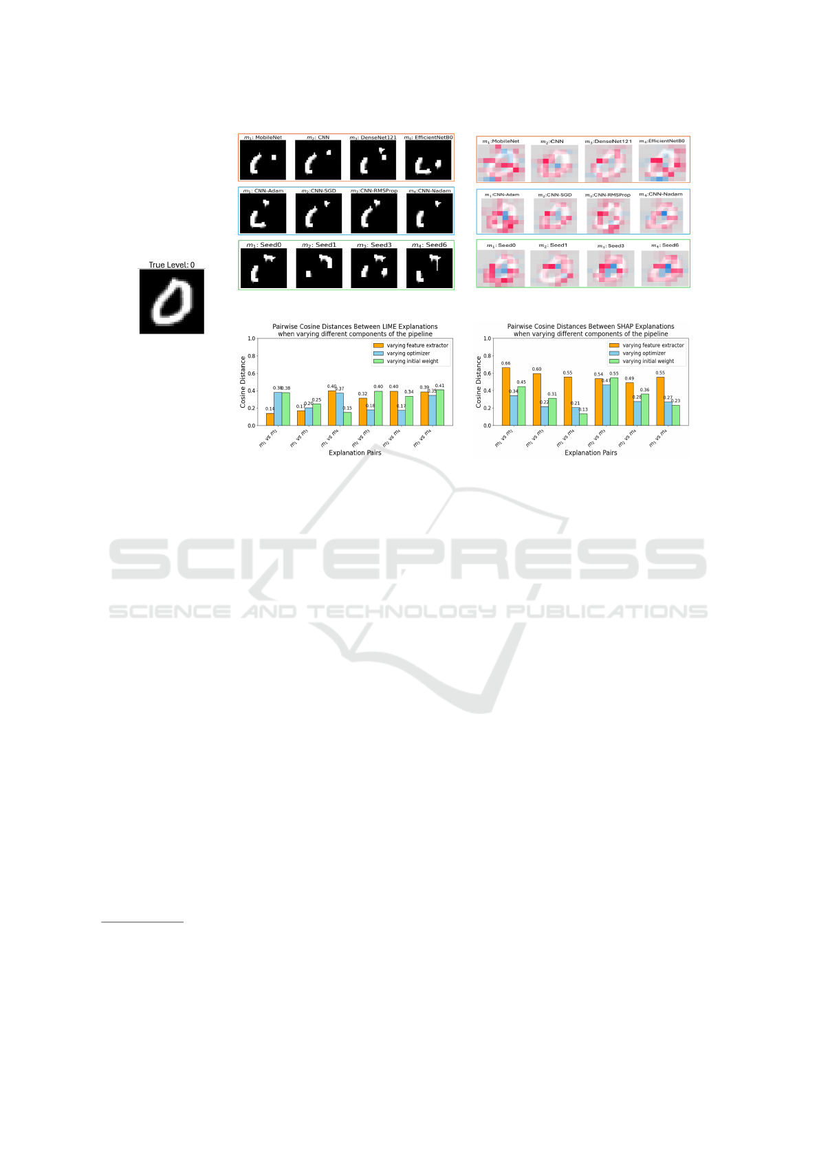
(a) Test image
(b) LIME explanations
(c) Variation on LIME explanations
(d) SHAP explanations
(e) Variation on SHAP explanations
Figure 3: Instance-level experiments with varying pipeline components for a test input (a). (b) and (d) show LIME and
SHAP explanations clustered by component: top (orange border), middle (skyblue border), and bottom (green border) rows
represent the feature extractor, optimizer, and weight initialization, respectively. (c) and (e) summarize statistical variations
using color-coded bar plots matching the rows in (b) and (d).
est variability for this component. Since these re-
sults are based on a single instance, they may not
fully capture the broader variation in model behavior.
Therefore, class-level quantification is necessary to
assess the true impact of feature extractor variations.
In contrast, variations in the “optimizer” and “ini-
tial weights” (Figure 3) resulted in less pronounced,
though still observable differences in the highlighted
regions. These variations suggest that even subtle
changes, such as optimization strategies or initializa-
tion seeds, can influence how the model interprets and
assigns importance to features for a specific instance.
4
Class-level underspecification analyzes the con-
sistency of feature importance explanations across
classes. Our analysis across all three datasets and ex-
planation methods, supports our instance-level analy-
sis and reveals that varying the feature extractor leads
to the highest average ClassLevelScore across classes,
indicating the greatest variability in feature reliance
(Figure 4, orange bars). This inconsistency suggests
that the choice of feature extractor is a primary fac-
tor in underspecification, as differences in architec-
4
We focus on presenting instance-level analysis only
for MNIST due to space constraints and its limited infor-
mativeness compared to class-level analysis. Extending to
other datasets would add redundancy without significant ad-
ditional value.
ture result in distinct feature representations and sig-
nificant shifts in feature importance and reliance.
In contrast, variations in the optimizer and initial
weights produced lower average ClassLevelScore (the
blue and green bars in Figure 4), reflecting reduced
variability in explanations. Although these variations
were smaller, they suggest that optimizers and initial-
ization seeds do play pivotal roles in underspecifica-
tion.
Overall, these findings highlight that while fea-
ture extractors are a dominant factor in the occur-
rence of underspecification in ML pipelines, each
component has the potential to introduce some degree
of underspecification. This underscores the impor-
tance of carefully considering all components in the
model pipeline to reduce underspecification and im-
prove model interpretability and robustness.
4.2.3 Time Complexity Analysis
Our proposed framework involves three main steps,
each contributing to the overall time complexity:
• Pipeline Modeling and Training: Let m be the
number of variations for a selected component,
and let T denote the average training time for each
model. The complexity for training all m models
is: O(m · T ).
A Framework for Identifying Underspecification in Image Classification Pipeline Using Post-Hoc Analyzer
433

(a) LIME explanation variations across different datasets
(b) SHAP explanation variations across different datasets
Figure 4: Class-Level Explanation Inconsistency across Pipeline Components for all Three Datasets. (a) LIME expla-
nation variations (left column) for MNIST (top), Imagenette (middle), and Cats vs Dogs (bottom). (b) SHAP explanation
variations (right column) for the same datasets. Bars indicate the impact of varying key pipeline components: feature extrac-
tor (orange), optimizer (sky blue), and initial weights (light green).
• Explanation Generation: We employ LIME and
SHAP on each of the k models to explain N test
instances. Let e represent the number of pertur-
bations or evaluations needed per instance. Con-
sequently, the complexity of generating explana-
tions is:
O(k · N · e)
• Underspecification Measurement: To compare
explanations across different models, we compute
pairwise distances. Since there are

k
2

=
k(k−1)
2
pairs among k models, and we perform these com-
parisons for N instances, the overall complexity is
on the order of:
O(k
2
· N)
Putting it all together, the total time complexity of
the framework can be expressed as:
O

m · T
|
{z}
model training
+ k · N · e
| {z }
explanation generation
+ k
2
· N
|{z}
calculation

In practical settings, the explanation generation
step (O(k · N · e)) often dominates, especially if
e (the number of perturbations or evaluations) is
large, if the black-box models are expensive to
query.
5 CONCLUSION
We introduce a framework to systematically exam-
ine how different ML pipeline components con-
tribute to underspecification by evaluating feature re-
liance through post-hoc explanation tools, specifi-
ICPRAM 2025 - 14th International Conference on Pattern Recognition Applications and Methods
434

cally LIME and SHAP. Our experiments reveal that
models with similar and high accuracy can rely on
different features — potentially spurious and irrel-
evant ones — in the decision-making process, em-
phasizing that high accuracy alone does not guaran-
tee model reliability. Among the components tested,
varying the feature extractor introduced the highest
variability in feature reliance, identifying it as the pri-
mary factor in underspecification. However, optimiz-
ers and initial weights can also contribute to under-
specification. While this study primarily focuses on
these three components, our proposed framework can
be extended to investigate additional elements within
ML pipelines.
While this study effectively highlights the preva-
lence of underspecification in various ML pipeline
components and identifies where it potentially occurs,
it is important to note that it does not directly address
how to reduce it. Additionally, we observe slight in-
consistencies in LIME explanations due to its inher-
ent randomness, which suggests that relying solely
on LIME may limit the robustness of underspecifica-
tion analysis. Additionally, our cosine distance-based
ClassLevelScore metric, despite its effectiveness, dis-
plays sensitivity on simpler datasets like MNIST, po-
tentially amplifying variability and underspecification
in these cases. Furthermore, while dataset quality
and representation are known to significantly impact
underspecification, these aspects are not directly ex-
plored in this work, as they are extensively studied
in the literature. Lastly, although post-hoc explana-
tion tools such as LIME and SHAP provide valuable
insights, their computational intensiveness may limit
their applicability to datasets with large numbers of
classes or instances, posing a challenge for scalability
in more complex settings.
Future work will focus on addressing these limi-
tations by exploring strategies to mitigate underspec-
ification. This may involve identifying which feature
extractors or optimizers contribute most consistently
to stable feature reliance, testing alternative initializa-
tion methods, and developing a framework to guide
pipeline configurations toward reduced variability.
REFERENCES
Alahmari, S. S., Goldgof, D. B., Mouton, P. R., and Hall,
L. O. (2020). Challenges for the repeatability of deep
learning models. IEEE Access, 8:211860–211868.
Arnold, C., Biedebach, L., K
¨
upfer, A., and Neunhoeffer,
M. (2024). The role of hyperparameters in machine
learning models and how to tune them. Political Sci-
ence Research and Methods, 12(4):841–848.
Bischl, B., Binder, M., Lang, M., Pielok, T., Richter,
J., Coors, S., Thomas, J., Ullmann, T., Becker, M.,
Boulesteix, A.-L., et al. (2023). Hyperparameter op-
timization: Foundations, algorithms, best practices,
and open challenges. Wiley Interdisciplinary Reviews:
Data Mining and Knowledge Discovery, 13(2):e1484.
Bouthillier, X., Delaunay, P., Bronzi, M., Trofimov, A.,
Nichyporuk, B., Szeto, J., Sepah, N., Raff, E., Madan,
K., Voleti, V., et al. (2021). Accounting for vari-
ance in machine learning benchmarks. arXiv preprint
arXiv:2103.03098.
Breiman, L. (2001). Statistical modeling: The two cultures
(with comments and a rejoinder by the author). Sta-
tistical science, 16(3):199–231.
Chollet, F. (2017). Xception: Deep learning with depthwise
separable convolutions. In Proceedings of the IEEE
conference on computer vision and pattern recogni-
tion, pages 1251–1258.
D’Amour, A., Heller, K., Moldovan, D., Adlam, B., Ali-
panahi, B., Beutel, A., Chen, C., Deaton, J., Eisen-
stein, J., Hoffman, M. D., et al. (2022). Underspeci-
fication presents challenges for credibility in modern
machine learning. Journal of Machine Learning Re-
search, 23(226):1–61.
Dozat, T. (2016). Incorporating nesterov momentum into
adam. Technical report, Stanford University.
He, K., Zhang, X., Ren, S., and Sun, J. (2016). Identity
mappings in deep residual networks. In Computer
Vision–ECCV 2016: 14th European Conference, Am-
sterdam, The Netherlands, October 11–14, 2016, Pro-
ceedings, Part IV 14, pages 630–645. Springer.
Hinns, J., Fan, X., Liu, S., Raghava Reddy Kovvuri, V., Yal-
cin, M. O., and Roggenbach, M. (2021). An initial
study of machine learning underspecification using
feature attribution explainable ai algorithms: A covid-
19 virus transmission case study. In PRICAI 2021:
Trends in Artificial Intelligence: 18th Pacific Rim In-
ternational Conference on Artificial Intelligence, PRI-
CAI 2021, Hanoi, Vietnam, November 8–12, 2021,
Proceedings, Part I 18, pages 323–335. Springer.
Hinton, G. (2012). Lecture 6e rmsprop: Divide the gradient
by a running average of its recent magnitude. Cours-
era Lecture: Neural Networks for Machine Learning.
Howard, A. G., Zhu, M., Chen, B., Kalenichenko, D.,
Wang, W., Weyand, T., Andreetto, M., and Adam,
H. (2017). Mobilenets: Efficient convolutional neu-
ral networks for mobile vision applications. arXiv
preprint arXiv:1704.04861.
Howard, J. (2019). Imagenette (version 1.0). https://github
.com/fastai/imagenette. GitHub repository.
Huang, G., Liu, Z., Van Der Maaten, L., and Weinberger,
K. Q. (2017). Densely connected convolutional net-
works. In Proceedings of the IEEE conference on
computer vision and pattern recognition, pages 4700–
4708.
Kaggle (2013). Dogs vs. Cats Dataset. https://www.kaggle
.com/c/dogs-vs-cats. Accessed: 2024-11-09.
Kamath, U. and Liu, J. (2021). Explainable artificial in-
telligence: an introduction to interpretable machine
learning, volume 2. Springer.
A Framework for Identifying Underspecification in Image Classification Pipeline Using Post-Hoc Analyzer
435

Kingma, D. P. (2014). Adam: A method for stochastic op-
timization. arXiv preprint arXiv:1412.6980.
Lakshminarayanan, B., Pritzel, A., and Blundell, C. (2017).
Simple and scalable predictive uncertainty estimation
using deep ensembles. Advances in neural informa-
tion processing systems, 30.
LeCun, Y., Bottou, L., Bengio, Y., and Haffner, P. (1998).
Gradient-based learning applied to document recogni-
tion. Proceedings of the IEEE, 86(11):2278–2324.
Li, B., Qi, P., Liu, B., Di, S., Liu, J., Pei, J., Yi, J., and
Zhou, B. (2023). Trustworthy ai: From principles to
practices. ACM Computing Surveys, 55(9):1–46.
Lundberg, S. M. and Lee, S.-I. (2017). A unified approach
to interpreting model predictions. Advances in neural
information processing systems, 30.
Madras, D., Atwood, J., and D’Amour, A. (2019). Detect-
ing underspecification with local ensembles. arXiv
preprint arXiv:1910.09573.
Mehrer, J., Spoerer, C. J., Kriegeskorte, N., and Kietz-
mann, T. C. (2020). Individual differences among
deep neural network models. Nature communications,
11(1):5725.
Molnar, C. (2020). Interpretable machine learning. Lulu.
com.
M
¨
uller, S., Toborek, V., Beckh, K., Jakobs, M., Bauckhage,
C., and Welke, P. (2023). An empirical evaluation of
the rashomon effect in explainable machine learning.
In Joint European Conference on Machine Learning
and Knowledge Discovery in Databases, pages 462–
478. Springer.
Ovadia, Y., Fertig, E., Ren, J., Nado, Z., Sculley, D.,
Nowozin, S., Dillon, J., Lakshminarayanan, B., and
Snoek, J. (2019). Can you trust your model’s uncer-
tainty? evaluating predictive uncertainty under dataset
shift. Advances in neural information processing sys-
tems, 32.
Qui
˜
nonero-Candela, J., Sugiyama, M., Schwaighofer, A.,
and Lawrence, N. D. (2022). Dataset shift in machine
learning. Mit Press.
Ribeiro, M. T., Singh, S., and Guestrin, C. (2016). ” why
should i trust you?” explaining the predictions of any
classifier. In Proceedings of the 22nd ACM SIGKDD
international conference on knowledge discovery and
data mining, pages 1135–1144.
Ruder, S. (2016). An overview of gradient de-
scent optimization algorithms. arXiv preprint
arXiv:1609.04747.
Szegedy, C., Vanhoucke, V., Ioffe, S., Shlens, J., and Wo-
jna, Z. (2016). Rethinking the inception architecture
for computer vision. In Proceedings of the IEEE con-
ference on computer vision and pattern recognition,
pages 2818–2826.
Tan, M. and Le, Q. (2019). Efficientnet: Rethinking model
scaling for convolutional neural networks. In Interna-
tional conference on machine learning, pages 6105–
6114. PMLR.
Teney, D., Peyrard, M., and Abbasnejad, E. (2022). Predict-
ing is not understanding: Recognizing and address-
ing underspecification in machine learning. In Euro-
pean Conference on Computer Vision, pages 458–476.
Springer.
ICPRAM 2025 - 14th International Conference on Pattern Recognition Applications and Methods
436