Quantum Multi-Agent Reinforcement Learning for Aerial Ad-Hoc
Networks
Theodora-Augustina Dr
˘
agan
1
, Akshat Tandon
2 a
, Tom Haider
1 b
, Carsten Strobel
2 c
,
Jasper Simon Krauser
2
and Jeanette Miriam Lorenz
1 d
1
Fraunhofer Institute for Cognitive Systems IKS, Munich, Germany
2
Airbus Central Research & Technology, Ottobrunn, Germany
Keywords:
Quantum Multi-Agent Reinforcement Learning, Proximal Policy Optimization, Communication, Networks.
Abstract:
Quantum machine learning (QML) as combination of quantum computing with machine learning (ML) is
a promising direction to explore, in particular due to the advances in realizing quantum computers and the
hoped-for quantum advantage. A field within QML that is only little approached is quantum multi-agent
reinforcement learning (QMARL), despite having shown to be potentially attractive for addressing industrial
applications such as factory management, cellular access and mobility cooperation. This paper presents an
aerial communication use case and introduces a hybrid quantum-classical (HQC) ML algorithm to solve it.
This use case intends to increase the connectivity of flying ad-hoc networks and is solved by an HQC multi-
agent proximal policy optimization algorithm in which the core of the centralized critic is replaced with a
data reuploading variational quantum circuit. Results show a slight increase in performance for the quantum-
enhanced solution with respect to a comparable classical algorithm, earlier reaching convergence, as well as
the scalability of such a solution: an increase in the size of the ansatz, and thus also in the number of trainable
parameters, leading to better outcomes. These promising results show the potential of QMARL to industrially-
relevant complex use cases.
1 INTRODUCTION
In the field of aerospace communication, technology
has already enabled wireless mobile nodes to connect
to each other and to act as both relay points and ac-
cess points. This allows the creation of flying ad-hoc
networks (FANET). Architectural advancements have
recently been made in this field, such as free-space
optical communication (FSO) hardware, as well as
the corresponding communication management soft-
ware (Helle et al., 2022b; Helle et al., 2022a). This
means that the FANETs, which were usually made
up of unmanned aerial vehicles (UAV), can now be
formed by commercial aircrafts, satellites, as well as
by other platforms, enabling them to exchange infor-
mation. The main challenges of FANETs, when com-
pared to other types of ad-hoc networks, are the high
a
https://orcid.org/0000-0001-8588-2927
b
https://orcid.org/0000-0001-6786-0361
c
https://orcid.org/0000-0001-6608-0232
d
https://orcid.org/0000-0001-6530-1873
mobility degree and the low node density, which ren-
ders link disconnections and network partitions more
likely (Khan et al., 2020).
The FANET nodes can therefore collaborate to
overcome the connectivity challenge by addressing it
as a common goal. Each node can choose which other
nodes to open a communication channel with, such
that as many nodes as possible are directly or indi-
rectly reachable by the rest of the network. There are
several benefits for aircrafts to create ad-hoc networks
that motivate this work, such as for passenger and air-
craft connectivity, as well as for acting as a backbone
for internet service providers. For this purpose, a cen-
tralized decision-making process would be able to ap-
ply fully-informed routing protocols and dynamically
adjust connections as topology changes. While such
strategies perform better than a collection of random
agents, they are impractical in FANETs: they do not
scale well with a large number of network nodes and
become impractical, and thus decentralized solutions
are preferable (Khan et al., 2020; Helle et al., 2022a;
Kim et al., 2023).
Dr
ˇ
agan, T.-A., Tandon, A., Haider, T., Strobel, C., Krauser, J. S. and Lorenz, J. M.
Quantum Multi-Agent Reinforcement Learning for Aerial Ad-Hoc Networks.
DOI: 10.5220/0013375100003890
Paper published under CC license (CC BY-NC-ND 4.0)
In Proceedings of the 17th International Conference on Agents and Artificial Intelligence (ICAART 2025) - Volume 1, pages 731-741
ISBN: 978-989-758-737-5; ISSN: 2184-433X
Proceedings Copyright © 2025 by SCITEPRESS – Science and Technology Publications, Lda.
731

Multi-agent reinforcement learning (MARL) is a
collection of methods designed for multi-agent sys-
tems (MAS). They assume that each agent is a differ-
ent entity which can learn how to behave in an en-
vironment by interacting with it. It usually entails
two processes: training, when the agents update their
internal rules depending on the feedback caused by
their actions, and execution, when they act according
to those rules. MARL could provide here a solution,
as it contains algorithms where the agents could use
global information during training, and only local in-
formation during execution. The advantage of these
methods is the reduction in inter-agent communica-
tion overhead. However, this paradigm comes with
certain drawbacks, such as the poor scalability, a high
demand of computational resources, as well as only
having partial access to environmental information.
Therefore, we explore if a quantum-enhanced MARL
(QMARL) could help to tackle some of these issues
and could lead to a better performance of the agents.
The contributions detailed in this work are:
• We present an HQC multi-agent proximal pol-
icy optimization algorithm, where the core of the
centralized critic is a data reuploading variational
quantum circuit (VQC). The VQC is designed so
that it is compatible with the quantum technology
currently available.
• We model an aerial communication use case
against which both the aforementioned HQC
MARL algorithm and its classical counterpart are
benchmarked.
• We scale up the size of the VQC with respect
to the number of layers and, respectively, the
complexity of the use case, and assess the scal-
ability of our solution. We also characterize the
VQC using two quantum metrics that are well-
motivated by literature, namely expressibility and
entanglement capability. The purpose is to ob-
serve whether any correlation could be drawn be-
tween the performance of the HQC solution and
the embedded quantum module.
This paper is structured as follows: the next sec-
tion is a dive into the theoretical basis notions of
MARL, followed by a presentation of the current state
of the art in QMARL. The fourth section presents the
MARL environment, therefore the task at hand, while
section 5 details the classical MARL algorithm the
solution is built on and the process of embedding a
quantum kernel into the training process. In section 6
we introduce the methods for evaluating the classi-
cal and quantum solutions with respect to their per-
formance, as well as to their architectural properties.
In section 7 we present the results of the QMARL so-
lution and then draw the conclusions in the final chap-
ter.
2 BACKGROUND
In this section, we will introduce the (MA)RL
paradigm and its applications, as well as the main
challenges encountered in the development of such
algorithms and the main categories in which they are
divided. Finally, we present the method we chose to
build our QMARL algorithm on.
MARL is a collection of methods which make
use of the reinforcement learning (RL) paradigm
in order to enable agents to successfully behave in
MASs. While supervised and unsupervised ML pro-
pose training a model on input data in order to per-
form a task, RL agents interact with their environ-
ment and observe the feedback they get as reward in
order to improve their behaviour in the environment
and obtain better rewards. These methods applied to
MAS contexts can achieve results comparable to pro-
fessional human players in video games (Ellis et al.,
2023), as well as perform well on industrially-relevant
use cases such as smart manufacturing (Bahrpeyma
and Reichelt, 2022), UAV cooperation for network
connectivity and path planning (Qie et al., 2019),
and energy scheduling of residential microgrid (Fang
et al., 2019).
The ubiquity of MAS and extensive research of
RL methods motivated the development of existing
single-agent RL algorithms into MARL solutions.
However, this yielded new challenges: since the state
of an environment does not depend on the actions of
a single agent, the environment is thus non-stationary
with respect to that agent. Scalability and the curse
of dimensionality are also characteristics of MARL,
since the dimensions of the joint state and action
spaces can steeply increase and thus make solutions
demand more computational resources. Finally, most
environments are only partially observable for each
agent, while RL algorithms assume the agent has full
knowledge of the environment.
In a MARL solution there are two stages, train-
ing, when the model of the behaviour of each agent
is updated through interactions with the environment,
and execution, when a trained model starts perform-
ing its assigned task in the environment. Depending
on whether information is shared between the agents
during each of these two stages, three approaches can
be distinguished:
• Centralized training, centralized execution
(CTCE): agents are always able to communicate
and can be viewed as one single agent. The draw-
QAIO 2025 - Workshop on Quantum Artificial Intelligence and Optimization 2025
732

back of this approach is that agents are expected
to exchange information during execution, which
decreases scalability and increases overhead.
• Decentralized training, decentralized execution
(DTDE): agents never communicate and act as in-
dependent RL single agents. While this option
has little overhead in both the development and
the testing of the solutions, it also underperforms
when compared to other approaches.
• Centralized training, decentralized execution
(CTDE): agents are able to communicate during
the training process, for example by having ac-
cess to simulator information or by communicat-
ing through a network. During execution, infor-
mation is not shared anymore.
We chose to implement an algorithm of the CTDE
approach, since this paradigm is able to help miti-
gate the scalability and the partial observability is-
sues. Since knowledge sharing only happens during
training, agents may learn better than by only hav-
ing local information, but they also avoid the infor-
mational exchange overhead during execution, where
they act as single agents.
3 RELATED WORKS
This section provides an introduction into the present
advancements in the field of QMARL. We start with
a general presentation of quantum methods in ML
and in RL, and then present the possible paths of de-
velopment of quantum-enhanced solutions. We then
conclude with a presentation of the current status of
QMARL approaches through selected works.
Quantum machine learning is a collection of
methods that can be found at the intersection between
quantum computing and machine learning. In this
work, we understand it as using quantum phenom-
ena such as superposition, entanglement, and infer-
ence in order to gain a computational advantage or a
better performance on applications where input data is
classical. The motivation behind this field is the fact
that methods with quantum modules were shown to
have lower time complexities (Wiebe et al., 2014; Li
et al., 2022; Lloyd et al., 2013), better performances
with respect to the application-specific metrics (Ullah
et al., 2022; Abbas et al., 2021), as well as theoretical
advantages, such as a better generalization in cases
where data samples are limited (Caro et al., 2022).
These aspects also apply to quantum reinforce-
ment learning (QRL), where several works already
proposed multiple directions (Meyer et al., 2024).
These can be divided into four main pillars: quantum-
inspired methods(classical algorithms that mimic
quantum principles), VQC-based function approxi-
mators, RL algorithms with quantum methods, and
fully-quantum RL. The second category comprises
the only algorithms with quantum modules that are
suitable for the currently available quantum hard-
ware, also known as noisy intermediate-scale quan-
tum (NISQ) devices (Preskill, 2018). The VQC-based
subdomain contains classical RL algorithms that orig-
inally use neural networks (NN) as function approxi-
mators and now replaced them with VQCs. Such so-
lutions were already proposed for use cases such as
robotics (Heimann et al., 2022), wireless communi-
cation (Chen et al., 2020), optimization (Skolik et al.,
2023), and logistics (Correll et al., 2023). In such
works, VQCs can be employed in order to compute
the suitability of an environmental state, the probabil-
ities of an action to be taken in a given state, or other
intermediary computations that help the agent to suc-
cessfully navigate the environment.
Most of the QMARL literature also focuses on
these VQC-based NISQ-friendly algorithms. For ex-
ample, an actor-critic QMARL algorithm was applied
on two cooperative tasks: smart factory management
and mobile access generated by UAVs (Park et al.,
2023b; Yun et al., 2023). Three types of solutions
were proposed, depending on the implementation of
the actor and, respectively, of the centralized critic:
entirely quantum (QQ), a quantum-centralized critic
and classical actors (QC), and entirely classical (CC).
The VQCs of the QQ and QC solutions consisted of
an angle data encoding and a trainable layer of rota-
tional gates and CNOT entanglement gates. Results
show that the architecture of quantum actors and a
quantum critic learnt more efficiently than other ap-
proaches (Park et al., 2023b; Yun et al., 2023). For
comparable rewards to be achieved during training,
the classical approach would require two orders of
magnitude more trainable parameters. Moreover, if
projection value measure is used for dimensionality
reduction on the action space of the quantum solution,
it scales better than other classical algorithms once
the action space reaches the order of 2
16
. This hints
towards a better suitability of QMARL solutions for
industrially-relevant MAS use cases, when compared
to classical MARL.
A similar work makes use of quantum actors and a
quantum centralized critic in a realistic decentralized
environment of multi-UAV cooperation in the pres-
ence of noise (Park et al., 2023a). The actions of
the UAVs in that use case are their movements, which
should conduct to a better-performing UAV network
as observed by the end users on the ground. The
simulation environment is challenged through noise:
Quantum Multi-Agent Reinforcement Learning for Aerial Ad-Hoc Networks
733

generalised Cauchy state value noise and Weibull
distribution-like noise on the action values, which
render the simulation environment closer to a real use
case. The presence of environmental and action noise
is actually favorable for the QMARL solutions, which
then converge faster and to higher rewards than their
noiseless or classical counterparts.
Another hybridised paradigm present in literature
is evolutionary optimization, in which the optimiza-
tion of the parameter set of a model is done analo-
gously to natural selection. Several initial sets of po-
tential parameters are generated and then, in an iter-
ative process, the best candidates are selected based
on a fitness function. New candidate parameters are
generated, until a satisfactory set of parameters is
achieved. Such an optimization process can be em-
ployed to train the embedded VQC in a QMARL
model to solve a coin game in which both the state
space and the actions taken are discrete (K
¨
olle et al.,
2024): in a grid-like environment two agents compete
against each other in order to maximize the number
of coins collected. Multiple evolution strategies were
applied to the QMARL algorithm and were bench-
marked against similar solutions which employ in-
stead NNs. Results show that quantum-inspired meth-
ods are able to reach comparable results to classical
ones, while reducing the parameter count to half.
4 ENVIRONMENT
G
0
G
1
A
0
A
1
A
2
A
3
A
4
A
5
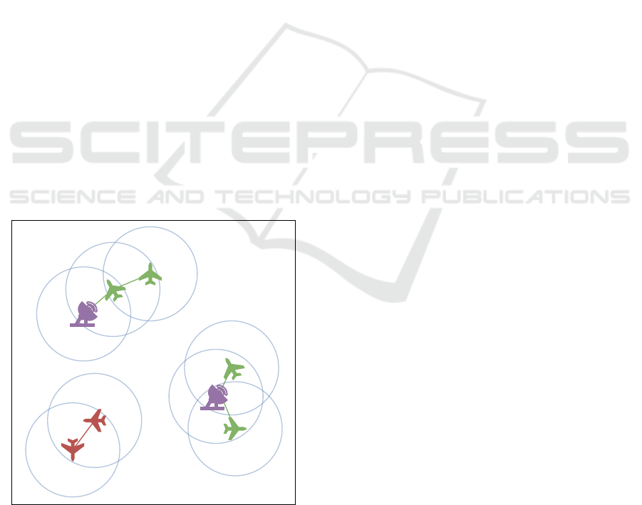
Figure 1: An environment of N = 8 entities: N
A
= 6 air-
crafts and N
G
= 2 ground stations.
To address inter-plane communication via both
MARL and QMARL algorithms, an environment to
simulate the aircrafts and ground stations needs to be
defined. This section introduces such an environment
from two points of view: the physical simulation of
the environment, as well as its mathematical formali-
sation as a partially-observable Markov decision pro-
cess.
The environment is a simulated MAS of several
entities, where an entity is either an aircraft or a
ground station. For each entity, its initial positions
and constant velocities on the x and y axes are ran-
domly and uniformly generated, with the velocities of
the ground stations being 0. Time is discretized into
time steps and at each time step the agents move ac-
cording to their velocities. Afterwards, they decide
who to connect to, as each of them is able to connect
to maximally 2 entities. If both agents decided to con-
nect to each other, the connection is established, else
not. The goal of the agents is to take good connection
decisions and create local ad-hoc networks such that
a maximally achievable number of aircrafts is con-
nected to the ground.
There are in total N = N
A
+ N
G
entities, where
N
A
is the number of aircrafts and N
G
is the number
of ground stations. An aircraft is connected to the
ground as long as it has an uninterrupted (multi-hop)
link to a ground station. For example, in the environ-
mental state shown in Fig. 1, aircrafts A
0
, A
2
and A
3
are connected directly to the ground stations G
0
and
G
1
, whereas A
1
is connected indirectly through A
0
.
Aircrafts A
4
and A
5
are connected to each other, but
as no other aircrafts or ground stations are in range,
they have no access to communication (where ranges
are represented through blue circles). A simulation is
run for T = 50 time steps, and the goal of each aircraft
is to properly choose to which other aircrafts to con-
nect in order to maximize the total number of aircrafts
connected to the ground.
The environment can be modelled as a decen-
tralized partially observed Markov decision process
(Dec-POMDP) (Oliehoek et al., 2016) denoted as
M = (D,S ,A,O,R, T ). In this notation, D =
{1,2,...,N
A
} is the set of agents, S is the set of states,
A is the set of joint actions, O is the set of observa-
tions, R is the immediate reward function and T is the
problem horizon.
In the following notations, all values correspond
to the properties of the environment at time step t, but
the index t is omitted for clarity purposes. The state
of the environment S = x
e
i
,y
e
i
,v
x
e
i
,v
y
e
i
1≤i≤N
contains
the x and y axis positions and the velocities of all enti-
ties {e
i
}
1≤i≤N
. The environment state S is not visible
to any of the entities, to reflect the real-world applica-
tion of such an environment.
The joint action set is A = {a
a
i
}
1≤i≤N
A
, where the
QAIO 2025 - Workshop on Quantum Artificial Intelligence and Optimization 2025
734

action a
a
i
of each aircraft a
i
is defined as:
a
a
i
= {c
e
0
,c
e
1
,...,c
e
N
}, (1)
where c
k
∈ (0,1) is a value directly proportionate to
how desirable the connectivity with entity e
k
̸= a
i
is to
the aircraft a
i
and the connectivity choice corresponds
to the highest 2 values.
The joint observation set is O = {o
a
i
}
1≤i≤N
A
,
where the observation o
a
i
of each aircraft a
i
is defined
as:
o
a
i
= {ptg
a
i
,ptg
e
1
,lk
e
1
,oc
e
1
,...,ptg
N−1
,lk
N−1
,oc
N−1
},
(2)
where ptg
e
k
= 1 if the entity e
k
̸= a
i
has a path to
the ground and ptg
e
k
= 0 otherwise. The normalized
link range lk
e
k
∈ [0,1] shows for how many steps, out
of the total number of simulated environmental time
steps, aircraft a
i
and entity e
k
will be in reach of each
other. If they are currently not in range, lk
e
k
= −1. Fi-
nally, the normalized occupied connections variable
oc
e
k
∈ [−1,1] indicates how many of the maximally
available connections are occupied. If oc
e
k
= −1, en-
tity e
k
has no active connections, and if oc
e
k
= 1 ,
it reached the maximal number of simultaneous con-
nections, which is set at two for the use case scenarios
tackled in this work.
The reward for each agent is chosen as a global
reward R:
R =
1
N
A
N
A
∑
i=1
ptg
i
, (3)
which is the averaged path to ground of all aircrafts at
a given time step t.
5 ALGORITHM
This chapter details the QMARL algorithm that
solves the environment defined in the previous sec-
tion. It is based on the multi-agent proximal policy
optimization (MAPPO) algorithm. The implemen-
tation was adapted from the MARLLib library (Hu
et al., 2023) and benchmarked against its classical
counterpart, both following the original MAPPO de-
sign (Yu et al., 2022), as described in Algorithm 1.
The MAPPO algorithm is the multi-agent version
of the proximal policy optimization (PPO) RL algo-
rithm (Schulman et al., 2017), which is widely used
in literature due to its performance on complex use
cases, such as robotics (Moon et al., 2022) and video
games (OpenAI et al., 2019). Like other actor-critic
RL algorithms, it uses two function approximators in
order to compute the next best action to be taken by
the agent. The actor, also known as the policy func-
tion, outputs the probabilities of each action to be
Initialize policies (actors) π
(a)
with
parameters θ
(a)
and the common critic V
with parameters φ;
Set learning rate α;
while step ≤ step
max
do
Set data buffer D = {};
for i = 1 to batch size do
Initialize trajectory τ = [];
for t = 1 to T do
for all agents a do
p
(a)
t
= π
(a)
(o
(a)
t
;θ
(a)
);
u
(a)
t
∼ p
(a)
t
;
v
(a)
t
= V (s
(a)
t
;φ);
end
Execute actions u
t
, observe
r
t
,s
t+1
,o
t+1
;
τ+ = [s
t
,o
t
,u
t
,r
t
,s
t+1
,o
t+1
];
end
Compute advantage estimate
ˆ
A on τ;
Compute reward-to-go
ˆ
R on τ;
Split trajectory τ into chunks of
length L;
for l = 0,1,...,T //L do
D = D ∪ (τ[l : l + T ],
ˆ
A[l : l + L],
ˆ
R[l : l + L]);
end
end
for mini-batch k = 1,...,K do
b ← random mini-batch from D with
all agent data;
Adam update θ on L(θ) with data b;
Adam update φ on L(φ) with data b;
end
end
Algorithm 1: The (Q)MAPPO training algorithm for
one agent (Yu et al., 2022). It is the same procedure for
both approaches, with the exception that in the MARL
case, the common critic V is entirely a NN, whereas in
QMARL it has a VQC core.
taken in a state. The critic, also known as the value
function, estimates the value of a given state of the
environment, directly proportional to the expected re-
ward to be obtained during the episode from that state
onwards. These two function approximators are usu-
ally implemented as NNs, in order to accommodate
for state and action spaces of high dimensions. The
main improvement brought by PPO in the actor-critic
family is using trust region policy updates with first-
order methods, as well as clipping the objective func-
tion. This enables the method to be more general than
other trust region policy methods and have a lower
sample complexity (Schulman et al., 2017).
Quantum Multi-Agent Reinforcement Learning for Aerial Ad-Hoc Networks
735

The MAPPO maintains the same architecture of
the PPO, with two types of NNs: the individual policy
π
θ
(actor) of each agent and the collective value func-
tion V
φ
(O) (critic), where O is the global environmen-
tal observation of the Dec-POMDP. The final goal of
our solution is to maximize the mean path to ground
at each time step, reflected by minimizing the cumu-
lative reward (CR) of all agents during an episode:
CR = T ∗ N
A
∗ R. (4)
In order to achieve this, the MAPPO algorithm
minimizes two losses through two Adam optimiz-
ers (Kingma and Ba, 2017), during the same training
process (Yu et al., 2022). The loss that the actor net-
work will minimize during training is:
L(θ) =
1
Bn
B
∑
i=1
n
∑
k=1

a
(k)
θ,i
+ σS[π
θ
(o
(k)
i
)]

, (5)
where a
(k)
θ,i
= min(r
(k)
θ,i
A
(k)
i
,clip(r
(k)
θ,i
,1 − ε,1 + ε)A
(k)
i
)
is the PPO-specific clipped advantage function A,
which can be understood as an estimated relative
value function, computed usually via generalized ad-
vantage estimation (GAE). Furthermore, θ is the pa-
rameter set of the actor network, B is the batch size,
n is the number of agents, S is the policy entropy, σ
is the entropy coefficient hyperparameter, and A
(k)
i
is
the advantage function.
The loss of the centralized critic is:
L(φ) =
1
Bn
B
∑
i=1
n
∑
k=1
max((V
φ
(o
(k)
i
) −
ˆ
R
i
)
2
,(v
(k)
φ,i
−
ˆ
R
i
)
2
).
(6)
In this case the clipped objective is the clipped
value function v
(k)
φ,i
= clip(V
φ
(o
(k)
i
),V
φ
old
(o
(k)
i
) −
ε,V
φ
old
(o
(k)
i
) + ε), φ is the parameter set of the critic
network and
ˆ
R
i
= γ
T
· CR is the discounted cumu-
lative reward. The values chosen for the MAPPO
hyperparameters in our implementation are found in
Table 1.
Table 1: Hyperparameter values.
Hyperparameter Value
GAE discount factor (λ
GAE
) 0.99
entropy factor (ε) 0.2
clipping factor (σ) 0.01
KL penalty 0.2
learning rate 0.0001
reward discount factor (γ) 0.99
5.1 Quantum Module
The hybrid quantum-classical variant of the MAPPO
(QMAPPO) algorithm we employ is obtained by re-
placing a part of the centralized critic NN with a
VQC, leaving the rest of the modules and the train-
ing policy intact. The critic NN has three parts: the
pre-processing block, the core block, and the post-
processing block. Each block is formed of fully-
connected linear layers followed by the hyperbolic
tangent activation function.
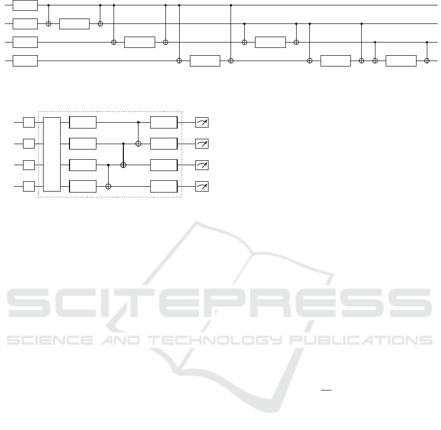
In the case of the QMAPPO solution, the core NN
block is replaced by a VQC, whose structure is dis-
played in Fig. 3. It is a data reuploading quantum
circuit of 4 qubits, which repeats L layers of a feature
map (FM) and of a trainable ansatz. The feature map
is a second-order Pauli-Z evolution circuit (the ZZ
feature map), in which the rotational angles are x
lq
i
=
f (o
lq
i
· ξ
lq
i
) and xx
lq
i
q
j
= 2(π − x
lq
i
)(π − x
lq
j
), where
l ∈ {0,1,2} is the layer index, q
i
,q
j
∈ {0,1,2,3},q
i
<
q
j
are input data indices in a layer 2, o are the pre-
processed input features, ξ are trainable input scaling
weights, and f is the pre-processing function, which
is either the identity or the inverse tangent function.
Depending on whether we repeat the feature map
for L = 1, 2 or 3 layers, we obtain VQC-1, VQC-2
and VQC-3 and embed then 4, 8, or, respectively, 12
features of the pre-processed input and thus the pre-
processing linear layer has an output dimension of
4,8 or 12 as well. When f is the identity function, so
no further scaling is applied, the circuits are referred
to as VQC-1N, VQC-2N and VQC-3N, and if f is the
inverse tangent function, they are referred to as VQC-
1A, VQC-2A and VQC-3A. The classical counter-
part of each VQC-based solution has a critic core NN
block of two hidden layers that have the same num-
ber of neurons. For a fair comparison, the number of
neurons per layer is chosen such that the total weight
count is as similar as possible between the MARL and
QMARL solutions, respectively. The classical solu-
tions are denoted as NN-X, where X is the number of
neurons in a hidden layer.
The Adam (Kingma and Ba, 2017) optimizer up-
dates all weights during training, using the first and
second moments of the gradient. In the case of the
quantum circuit, we chose to approximate the gradi-
ents through the simultaneous perturbation stochastic
approximation (SPSA) optimizer (Spall, 1998). This
decision is due to its efficiency: it needs only three cir-
cuit executions to output the gradients, whereas more
exact gradient methods, such as the parameter-shift-
rule, need O(2n) circuit executions.
6 EVALUATION
In this section we present the two types of metrics
that are used to benchmark all solutions: performance
metrics, which indicate how well the agents perform
QAIO 2025 - Workshop on Quantum Artificial Intelligence and Optimization 2025
736

R
Z
(x
l0
)
R
Z
(x
l1
) R
Z
(xx
l01
)
R
Z
(x
l2
) R
Z
(xx
l02
) R
Z
(xx
l12
)
R
Z
(x
l3
) R
Z
(xx
l03
) R
Z
(xx
l13
) R
Z
(xx
l23
)
Figure 2: Feature map (FM) of the variational quantum circuit, where xx
lq
i
q
j
is the rescaled encoding of classical features
with indices (4 ∗ l + q
i
) and (4 ∗ l + q
j
), with each layer l encoding four features on the four qubits q
0...3
.
|0⟩
H
F M
R
Y
(θ
l0
) R
Y
(θ
l4
)
|0⟩
H
R
Y
(θ
l1
) R
Y
(θ
l5
)
|0⟩
H
R
Y
(θ
l2
) R
Y
(θ
l6
)
|0⟩
H
R
Y
(θ
l3
) R
Y
(θ
l7
)
repeated for L layers
Figure 3: Structure of the VQC core of the centralized critic,
where FM is the feature map presented in Fig. 2 and θ
l0...7
are the respective trainable weights of each layer.
at evaluation during training, as well as architectural
metrics which are indicated by literature to give an
insight into the learning capability of a quantum-
enhanced solution.
6.1 Performance Metrics
In order to evaluate how well each architecture per-
forms, which is how well the agents choose commu-
nication links in environments of the same size they
were trained on, but of new configurations, we pro-
pose the following metrics:
• Maximal Cumulative Reward (MCR): the maxi-
mal value of the aggregated mean reward during
training across all experiments of a given solution,
sampled at evaluation;
• Converged Cumulative Reward (CCR): the mean
value of the aggregated mean reward during train-
ing across all experiments of a given solution af-
ter 10
6
time steps of training. This is proposed
since after 10
6
time steps, most solutions have
converged to a stable CR, therefore it can be seen
as a more robust average of the CR;
• Convergence Speed (CS): the number of thou-
sands of time steps it takes for a model to reach an
MCR 25% higher than the average CR achieved
by random agents (Rand).
6.2 Quantum Metrics
A significant endeavour in literature is to antici-
pate the performance of a quantum-enhanced solu-
tion and to compare between different solution ar-
chitectures on the same task (Bowles et al., 2024).
Among these architectural metrics, one may find the
trainability (McClean et al., 2018), the expressibil-
ity, the entanglement capability (Sim et al., 2019),
and the normalized effective dimension (Abbas et al.,
2021). Moreover, since most metrics are estimated on
sampled sets of the trainable parameters of a VQC
and can get computationally demanding, machine
learning-based estimating solutions were proposed as
well (Aktar et al., 2023). While clear correlations are
still to be found between any proposed metric and the
performance of the corresponding VQC-based solu-
tions, two quantum metrics are widely used in liter-
ature (Sim et al., 2019) and are presented in the re-
maining of this chapter: expressibility and entangle-
ment capability.
6.2.1 Entanglement Capability
The entanglement capability (Ent) of a VQC is an in-
dicator of how entangled its output states are (Sim
et al., 2019). This metric is based on the Meyer-
Wallach (MW) entanglement of a quantum state as
follows:
Ent =
1
|S|
∑
Θ
i
∈S
Q(ψ
i
), (7)
where Q(ψ
i
) is the MW entanglement applied to the
output quantum state ψ
i
, generated by a sampled vec-
tor of parameters Θ
i
∈ S, where S is the ensemble of
the sampled parameter vectors. The entanglement ca-
pability is bounded, Ent ∈ [0,1], and its value is di-
rectly proportional to how entangled the output states
are. For example e.g., Ent = 1 for a circuit that gener-
ates the maximally-entangled Bell states.
6.2.2 Expressibility
The expressibility (Expr) of a circuit is a quantum
metric that indicates how close the distribution of the
output states of that circuit is to the Haar ensemble, an
uniform distribution of random states. Therefore, it
measures how well a circuit covers the Hilbert space
and uses for this purpose the Kullback-Leibler (KL)
Quantum Multi-Agent Reinforcement Learning for Aerial Ad-Hoc Networks
737

divergence between the two distributions:
Exp = D
KL
(P
VQC
(F,Θ) || P
Haar
(F)), (8)
where P
PQC
is the estimated probability distribution of
the fidelities between pairs of samples of output states
of the VQC, P
Haar
= (N − 1)(1 − F)
N−2
is the proba-
bility distribution function between states of the Haar
ensemble, N is the dimension of the Hilbert space,
and F = |⟨ψ
θ
|ψ
φ
⟩|
2
is the fidelity function between
two quantum states |ψ
θ
⟩ and |ψ
φ
⟩.
The quantum metrics of each VQC were com-
puted using the qleet library (Azad and Sinha, 2023),
where they are implemented according to the defini-
tions given in this section. In the following section,
the results of the classical and QMARL models are in-
troduced and the latter are benchmarked against these
two quantum metrics.
7 RESULTS
To assess the scalability of the classical and quantum-
enhanced solutions with the complexity of the use
case, we benchmark them against two scenarios:
• 4A1S: A basic scenario of N = 5 entities, with
N
A
= 4 aircrafts and N
G
= 1 ground station. The
size of the observation of an agent is dim(o) =
13 and the action size of an agent is dim(a) = 4.
Therefore, the collective observation space is of
size dim(O) = 52 and the collective action size is
dim(a) = 16. The cumulative reward achieved by
random agents of uniformly generated actions is
CR
Rand
= 60.20.
• 5A2S: A more complex scenario of N = 7 en-
tities, with N
A
= 5 aircrafts and N
G
= 2 ground
stations. The size of the observation of an agent
is dim(o) = 19 and the action size of an agent is
dim(a) = 6. Therefore, the collective observation
space is of size dim(O) = 95 and the collective ac-
tion size is dim(a) = 24. The cumulative reward
achieved by random agents of uniformly gener-
ated actions is CR
Rand
= 84.88.
Three experiments are performed for each archi-
tecture – scenario pair. The models are trained for
1400000 time steps, where the random seeds of each
experiment are {0,1,2} and the CR is evaluated for
one episode every 1000 time steps. In Fig. 4 and in
Fig. 5 the results are plotted and smoothed using the
exponential moving average, with the error bands rep-
resenting the standard error of the three experiments.
Tables 2 and 3 present the aggregated results for all
chosen architectures and, respectively, performance
metrics, together with the number of classical, quan-
tum and total trainable weights.
When it comes to the smaller-scale 4A1S sce-
nario, all of the QMAPPO solutions with the in-
verse tangent input scaling function (VQC-1A, VQC-
2A, and VQC-3A) require around half as many iter-
ations to converge to the CR threshold of 75.25, and
they also obtain slightly higher MCR and compara-
ble CCR. Therefore, from Fig. 4 and Table 2, one can
conclude that a quantum-enhanced MAPPO solution
is better suited for the 4A1S scenario than a classi-
cal one that employs the same number of parameters,
especially with regards to the convergence speed, as
understood in this paper.
However, the hierarchy of suitability between so-
lutions is not the same for the 5A2S scenario. In
this case, the identity-scaled architectures are always
faster in terms of CS than the classical ones, but the
inverse tangent-scaled ones can, at times, perform
worse than the classical methods. For example, the
QMARL solution of three layers and no input scaling
needs slightly more time steps than the MARL solu-
tion to reach the MCR threshold of 106.1 established
for the CS metric.
The scalability of the VQC-based solution in both
scenarios can be seen in Fig. 4 and in Fig. 5. Both for
the identity-postprocessing solutions and the inverse
tangent-postprocessing solutions, as we increased the
number of reuploading layers, the CS of each archi-
tecture always decreased, while the MCR, and the CR
increased or remained at a comparable value. For the
5A2S scenario, in Table 3, the CCR slightly scales up
with the size of the solutions, but at no statistically
significant rate.
No clear correlations could be drawn when one
compares the quantum metrics of the VQCs with the
performance of the solutions they are embedded in.
Despite having lower entanglement and expressibility
values than the architectures where no input scaling
is applied, the inverse-tangent scaled solutions per-
formed better in terms of CS on the 4A1S scenario.
As the number of circuit layers increases for the HQC
solutions, the entanglement is reduced or stays con-
stant, while the expressibility follows no clear path.
Therefore, it is not clear if the entanglement capabil-
ity or the expressibility measures could provide hints
towards the scaling capabilities of QMARL solutions.
8 CONCLUSIONS
In this paper we introduced an aerial communication
use case, in which aircrafts need to choose which
communication links to create such that all aircrafts
which fulfill the physical constraints are connected to
base stations on the ground. Furthermore, we pro-
QAIO 2025 - Workshop on Quantum Artificial Intelligence and Optimization 2025
738

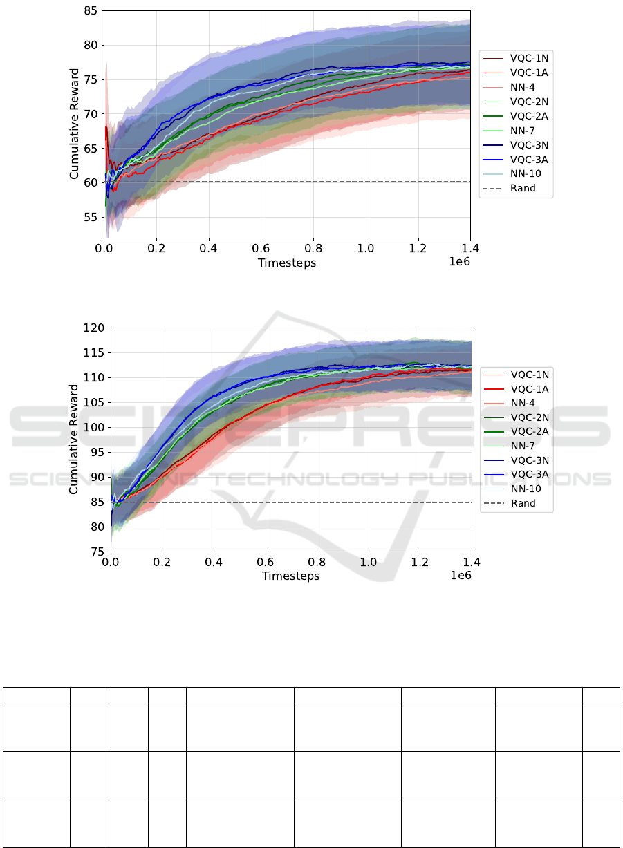
Figure 4: Smoothed aggregated cumulative reward at evaluation of all classical and QMARL solutions in the 4A1S scenario.
Figure 5: Smoothed aggregated cumulative reward at evaluation of all classical and QMARL solutions in the 5A2S scenario.
Table 2: The number of classical weights (CW), quantum weights (QW), and total weights (TW) of all solutions in the 4A1S
scenario, together with their respective expressibility (Expr) and entanglement capability (Ent), and their performance metrics:
maximal cumulative reward (MCR), converged cumulated reward (CCR), and converge speed (CS) in thousands of time steps.
Sol CW QW TW Expr Ent MCR CCR CS
NN-4 249 - 249 - - 84.23 ± 10.53 76.59 ± 3.78 255
VQC-1N 241 12 253 0.0013 ± 0.0001 0.8476 ± 0.0084 89.63 ± 6.26 77.91 ± 3.90 335
VQC-1A 241 12 253 0.0030 ± 0.0004 0.8043 ± 0.0091 89.93 ± 0.57 77.16 ± 5.09 203
NN-7 447 - 447 - - 86.56 ± 1.13 77.90 ± 3.91 195
VQC-2N 453 24 477 0.0012 ± 0.0002 0.8308 ± 0.0062 90.16 ± 3.05 78.01 ± 3.53 260
VQC-2A 453 24 477 0.0025 ± 0.0006 0.8128 ± 0.0091 87.43 ± 1.58 77.50 ± 3.91 141
NN-10 663 - 663 - - 87.76 ± 9.82 77.24 ± 4.30 215
VQC-3N 665 36 701 0.0013 ± 0.0002 0.8278 ± 0.0072 88.56 ± 9.15 78.01 ± 3.95 180
VQC-3A 665 36 701 0.0025 ± 0.0005 0.8186 ± 0.0076 89.76 ± 6.45 77.73 ± 4.08 133
Quantum Multi-Agent Reinforcement Learning for Aerial Ad-Hoc Networks
739

Table 3: The number of classical weights (CW), quantum weights (QW), and total weights (TW) of all solutions in the 5A2S
scenario, together with their respective expressibility (Expr) and entanglement capability (Ent), and their performance metrics:
maximal cumulative reward (MCR), converged cumulated reward (CCR), and converge speed (CS) in thousands of time steps.
Sol CW QW TW Expr Ent MCR CCR CS
NN-4 433 - 433 - - 119.93 ± 1.44 106.56 ± 5.76 360
VQC-1N 425 12 437 0.0013 ± 0.0001 0.8476 ± 0.0084 119.69 ± 1.51 107.28 ± 5.72 312
VQC-1A 425 12 437 0.0030 ± 0.0004 0.8043 ± 0.0091 125.23 ± 1.78 107.34 ± 6.55 246
NN-8 873 - 873 - - 122.13 ± 1.60 109.76 ± 4.49 210
VQC-2N 809 24 833 0.0012 ± 0.0002 0.8308 ± 0.0062 120.76 ± 5.14 109.81 ± 4.57 192
VQC-2A 809 24 833 0.0025 ± 0.0006 0.8128 ± 0.0091 121.56 ± 7.31 109.95 ± 4.60 202
NN-11 1224 - 1224 - - 121.03 ± 5.43 110.17 ± 4.31 181
VQC-3N 1193 36 1229 0.0013 ± 0.0002 0.8278 ± 0.0072 123.29 ± 7.76 111.02 ± 4.06 145
VQC-3A 1193 36 1229 0.0025 ± 0.0005 0.8186 ± 0.0076 121.96 ± 2.30 110.89 ± 3.93 186
posed a novel quantum-enhanced multi-agent proxi-
mal policy optimization algorithm, in which the core
of the centralized critic is implemented as a vari-
ational quantum circuit, which makes use of data
reuploading and of a second-order data embedding
scheme. Results show that the quantum-enhanced so-
lution outperforms the classical one in terms of max-
imal reward achieved at evaluation and of the conver-
gence speed, in number of training time steps. Nev-
ertheless, the fact that we could not draw the same
empirical correlations between the QMARL solutions
for the two scenarios of different complexities is an
argument towards the idea that quantum-enhanced so-
lutions need to be constructed and adapted to the spe-
cific use case they are to be applied on. Furthermore,
we attempted to apply quantum architectural metrics,
such as expressibility and entanglement, in order to
correlate performance to the architectural properties
of the quantum circuit. However, there were no clear
correlations present.
Future work on this topic could include scaling
the solution to a more complex and realistic use case,
as well as applying other quantum architectures and
compare suitability to the task. Furthermore, all re-
sults in this paper are obtained in a classical simula-
tion of a quantum system. Therefore, a possible de-
velopment branch would be to deploy this solution on
quantum hardware and observe the effect of the char-
acteristic noise and decoherence on the performance
of the solution. Finally, it remains an open ques-
tion and task to develop quantum architectural met-
rics that would offer an insight into the suitability of
a quantum-enhanced solution for a given task.
REFERENCES
Abbas, A., Sutter, D., Zoufal, C., Lucchi, A., Figalli,
A., and Woerner, S. (2021). The power of quan-
tum neural networks. Nature Computational Science,
1(6):403–409.
Aktar, S., B
¨
artschi, A., Badawy, A.-H. A., Oyen, D., and
Eidenbenz, S. (2023). Predicting expressibility of pa-
rameterized quantum circuits using graph neural net-
work. In 2023 IEEE International Conference on
Quantum Computing and Engineering (QCE). IEEE.
Azad, U. and Sinha, A. (2023). qleet: visualizing loss
landscapes, expressibility, entangling power and train-
ing trajectories for parameterized quantum circuits.
Quantum Information Processing, 22(6).
Bahrpeyma, F. and Reichelt, D. (2022). A review of
the applications of multi-agent reinforcement learn-
ing in smart factories. Frontiers in Robotics and AI,
9:1027340.
Bowles, J., Ahmed, S., and Schuld, M. (2024). Better than
classical? the subtle art of benchmarking quantum
machine learning models.
Caro, M. C., Huang, H.-Y., Cerezo, M., Sharma, K., Sorn-
borger, A., Cincio, L., and Coles, P. J. (2022). Gener-
alization in quantum machine learning from few train-
ing data. Nature communications, 13(1):4919.
Chen, S. Y.-C., Yang, C.-H. H., Qi, J., Chen, P.-Y., Ma,
X., and Goan, H.-S. (2020). Variational quantum cir-
cuits for deep reinforcement learning. IEEE Access,
8:141007–141024.
Correll, R., Weinberg, S. J., Sanches, F., Ide, T., and Suzuki,
T. (2023). Quantum neural networks for a supply
chain logistics application. Advanced Quantum Tech-
nologies, 6(7):2200183.
Ellis, B., Cook, J., Moalla, S., Samvelyan, M., Sun, M.,
Mahajan, A., Foerster, J., and Whiteson, S. (2023).
Smacv2: An improved benchmark for cooperative
multi-agent reinforcement learning. In Oh, A., Neu-
mann, T., Globerson, A., Saenko, K., Hardt, M., and
Levine, S., editors, Advances in Neural Information
Processing Systems, volume 36, pages 37567–37593.
Curran Associates, Inc.
Fang, X., Wang, J., Song, G., Han, Y., Zhao, Q., and Cao, Z.
(2019). Multi-agent reinforcement learning approach
for residential microgrid energy scheduling. Energies,
13(1):123.
Heimann, D., Hohenfeld, H., Wiebe, F., and Kirchner, F.
QAIO 2025 - Workshop on Quantum Artificial Intelligence and Optimization 2025
740

(2022). Quantum deep reinforcement learning for
robot navigation tasks.
Helle, P., Feo-Arenis, S., Shortt, K., and Strobel, C.
(2022a). Decentralized collaborative decision-making
for topology building in mobile ad-hoc networks. In
2022 Thirteenth International Conference on Ubiqui-
tous and Future Networks (ICUFN), pages 233–238.
Helle, P., Feo-Arenis, S., Strobel, C., and Shortt, K.
(2022b). Agent-based modelling and simulation of
decision-making in flying ad-hoc networks. In Ad-
vances in Practical Applications of Agents, Multi-
Agent Systems, and Complex Systems Simulation. The
PAAMS Collection, pages 242–253. Springer Interna-
tional Publishing.
Hu, S., Zhong, Y., Gao, M., Wang, W., Dong, H., Liang,
X., Li, Z., Chang, X., and Yang, Y. (2023). Marllib: A
scalable and efficient multi-agent reinforcement learn-
ing library.
Khan, M. F., Yau, K.-L. A., Noor, R. M., and Imran, M. A.
(2020). Routing schemes in fanets: A survey. Sensors,
20(1).
Kim, T., Lee, S., Kim, K. H., and Jo, Y.-I. (2023). Fanet
routing protocol analysis for multi-uav-based recon-
naissance mobility models. Drones, 7(3).
Kingma, D. P. and Ba, J. (2017). Adam: A method for
stochastic optimization.
K
¨
olle, M., Topp, F., Phan, T., Altmann, P., N
¨
ußlein, J., and
Linnhoff-Popien, C. (2024). Multi-agent quantum re-
inforcement learning using evolutionary optimization.
Li, J., Lin, S., Yu, K., and Guo, G. (2022). Quantum
k-nearest neighbor classification algorithm based on
hamming distance. Quantum Information Processing,
21(1):18.
Lloyd, S., Mohseni, M., and Rebentrost, P. (2013). Quan-
tum algorithms for supervised and unsupervised ma-
chine learning.
McClean, J. R., Boixo, S., Smelyanskiy, V. N., Babbush,
R., and Neven, H. (2018). Barren plateaus in quantum
neural network training landscapes. Nature communi-
cations, 9(1):4812.
Meyer, N., Ufrecht, C., Periyasamy, M., Scherer, D. D.,
Plinge, A., and Mutschler, C. (2024). A survey on
quantum reinforcement learning.
Moon, W., Park, B., Nengroo, S. H., Kim, T., and Har,
D. (2022). Path planning of cleaning robot with re-
inforcement learning.
Oliehoek, F. A., Amato, C., et al. (2016). A concise
introduction to decentralized POMDPs, volume 1.
Springer.
OpenAI, Berner, C., Brockman, G., Chan, B., Cheung,
V., Debiak, P., Dennison, C., Farhi, D., Fischer, Q.,
Hashme, S., Hesse, C., Jozefowicz, R., Gray, S., Ols-
son, C., Pachocki, J., Petrov, M., d. O. Pinto, H. P.,
Raiman, J., Salimans, T., Schlatter, J., Schneider, J.,
Sidor, S., Sutskever, I., Tang, J., Wolski, F., and
Zhang, S. (2019). Dota 2 with large scale deep re-
inforcement learning.
Park, C., Yun, W. J., Kim, J. P., Rodrigues, T. K., Park, S.,
Jung, S., and Kim, J. (2023a). Quantum multi-agent
actor-critic networks for cooperative mobile access in
multi-uav systems.
Park, S., Kim, J. P., Park, C., Jung, S., and Kim, J. (2023b).
Quantum multi-agent reinforcement learning for au-
tonomous mobility cooperation.
Preskill, J. (2018). Quantum computing in the nisq era and
beyond. Quantum, 2:79.
Qie, H., Shi, D., Shen, T., Xu, X., Li, Y., and Wang, L.
(2019). Joint optimization of multi-uav target assign-
ment and path planning based on multi-agent rein-
forcement learning. IEEE access, 7:146264–146272.
Schulman, J., Wolski, F., Dhariwal, P., Radford, A., and
Klimov, O. (2017). Proximal policy optimization al-
gorithms.
Sim, S., Johnson, P. D., and Aspuru-Guzik, A. (2019). Ex-
pressibility and entangling capability of parameter-
ized quantum circuits for hybrid quantum-classical al-
gorithms. Advanced Quantum Technologies, 2(12).
Skolik, A., Mangini, S., B
¨
ack, T., Macchiavello, C., and
Dunjko, V. (2023). Robustness of quantum reinforce-
ment learning under hardware errors. EPJ Quantum
Technology, 10(1):1–43.
Spall, J. C. (1998). An overview of the simultaneous pertur-
bation method for efficient optimization. Johns Hop-
kins apl technical digest, 19(4):482–492.
Ullah, U., Jurado, A. G. O., Gonzalez, I. D., and Garcia-
Zapirain, B. (2022). A fully connected quantum
convolutional neural network for classifying ischemic
cardiopathy. IEEE Access, 10:134592–134605.
Wiebe, N., Kapoor, A., and Svore, K. (2014). Quantum al-
gorithms for nearest-neighbor methods for supervised
and unsupervised learning.
Yu, C., Velu, A., Vinitsky, E., Gao, J., Wang, Y., Bayen,
A., and Wu, Y. (2022). The surprising effectiveness of
ppo in cooperative, multi-agent games.
Yun, W. J., Kim, J. P., Jung, S., Kim, J.-H., and Kim, J.
(2023). Quantum multi-agent actor-critic neural net-
works for internet-connected multi-robot coordination
in smart factory management.
Quantum Multi-Agent Reinforcement Learning for Aerial Ad-Hoc Networks
741