Upper Bound Computation for the Multiple Close-Enough Traveling

Salesman Problem

Francesco Carrabs

, Raffaele Cerulli

, Ciriaco D’Ambrosio

and Gabriele Murano

Department of Mathematics, University of Salerno, Giovanni Paolo II, 132, 84084, Fisciano(SA), Italy

{fcarrabs, raffaele, cdambrosio, gmurano}@unisa.it

Keywords:

Close-Enough, Multiple Traveling Salesman Problem, Neighborhoods, Drones.

Abstract:

This paper addresses the Multiple Close-Enough Traveling Salesman Problem, a variant of the Close-Enough

Traveling Salesman Problem, where multiple vehicles are used to visit a given number of points. A vehicle

visits a point if it passes through the neighborhood set of that point. The goal of the problem is to minimize

the longest of the deﬁned routes. We face the problem by using a discretization schema that reduces it to the

Multiple Generalized Traveling Salesman Problem for which we propose a Mixed Integer Linear Program-

ming formulation. The use of discretization schema introduces a discretization error that makes the optimal

solution value of our model an upper bound of the optimal solution value of the Multiple Close-Enough Trav-

eling Salesman Problem. Moreover, we apply a graph reduction algorithm to remove arcs and nodes without

changing the optimal solution of the problem. We provide proof of the correctness of this algorithm, and we

show that it signiﬁcantly reduces the size of the instances tested. We veriﬁed the performance of our model on

the benchmark instances of Close-Enough Traveling Salesman Problem.

1 INTRODUCTION

In this paper we address a variant of the Close-

Enough Traveling Salesman Problem (CETSP) called

the Multiple Close-Enough Traveling Salesman Prob-

lem (mCETSP). Given a set of target points in a Eu-

clidean space, where each target has a neighborhood

represented by a circular compact region centered on

the target, the CETSP consists of ﬁnding a minimum

length tour that starts and ends at a depot and inter-

sects each neighborhood once. The variant mCETSP

that, to the best of our knowledge, we address for

the ﬁrst time in the literature, considers m vehicles

and the neighborhoods are represented by a set of dis-

cretization points and it consists in ﬁnding m tours (or

routes), one for each vehicle, such that each neighbor-

hood is intersected by al least one tour. The goal of

the problem is to build the m tours so that the length

of the longest one is minimized.

The mCETSP has several practical applications in

the context of Unmanned Aerial Vehicles (UAV) in

particular when the use of multiple drones is required.

https://orcid.org/0000-0003-2187-8624

https://orcid.org/0000-0002-3277-6802

https://orcid.org/0000-0003-1274-6144

https://orcid.org/0009-0009-1238-1545

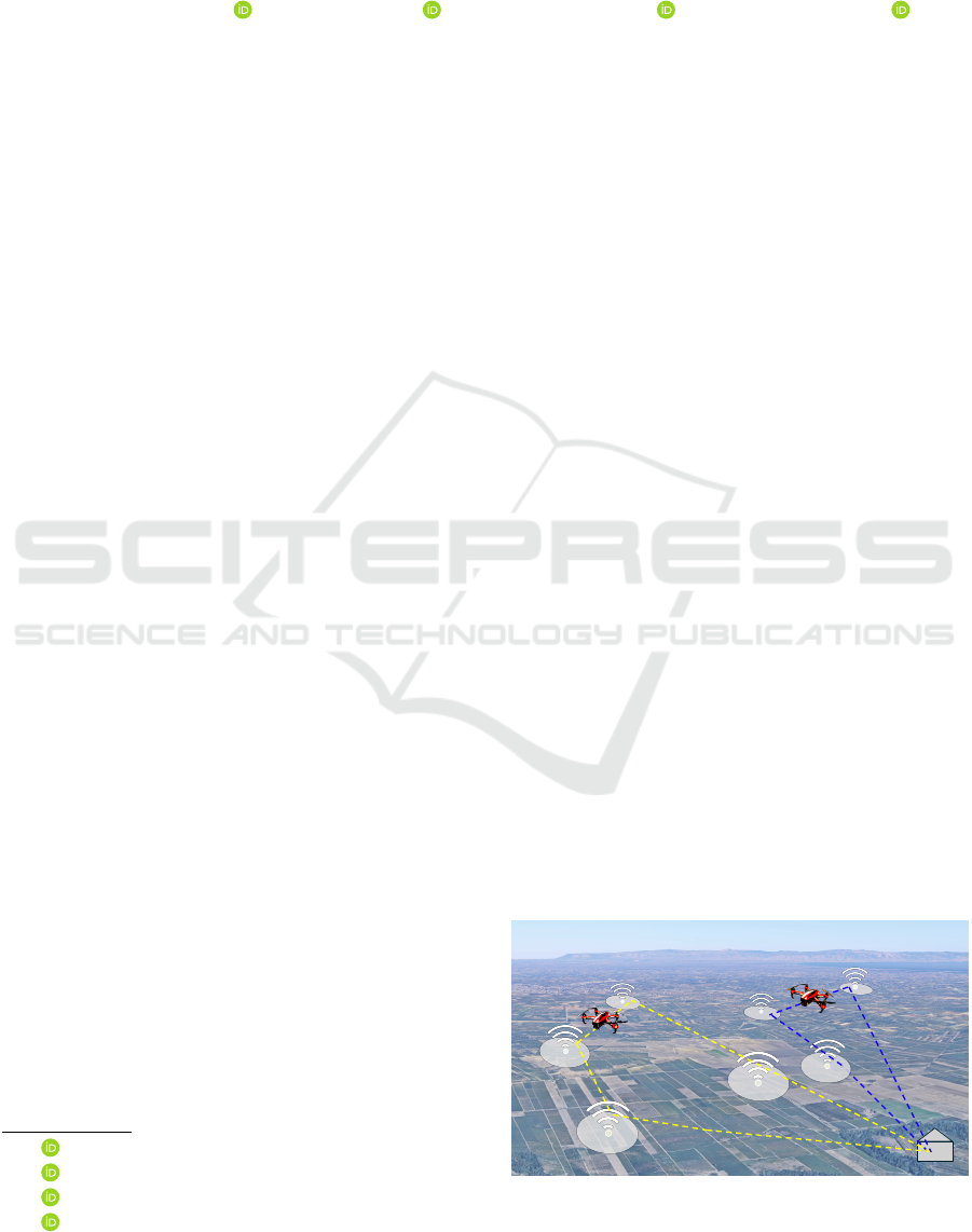
For example, in precision agriculture, a ﬂeet of drones

is tasked with ﬂying over speciﬁc areas of interest (see

Figure 1), gathering, from the sensors on the ground,

essential information on parameters such as soil mois-

ture, plant health, and other key indicators that inﬂu-

ence agricultural decisions. In such a context, it be-

comes essential to plan the routes of the drones so that

every area of interest is covered and the time to gath-

ering the information is minimized. A comprehensive

review of UAV applications in Smart Farming, along

with the critical role of route planning for these vehi-

cles, can be found in (Dolias et al., 2022).

The CETSP was deﬁned and addressed for the ﬁrst

time in (Gulczynski et al., 2006). The authors de-

Figure 1: Collecting information from ground sensors using

drones.

186

Carrabs, F., Cerulli, R., D’Ambrosio, C. and Murano, G.

Upper Bound Computation for the Multiple Close-Enough Traveling Salesman Problem.

DOI: 10.5220/0013377900003893

Paper published under CC license (CC BY-NC-ND 4.0)

In Proceedings of the 14th International Conference on Operations Research and Enterprise Systems (ICORES 2025), pages 186-195

ISBN: 978-989-758-732-0; ISSN: 2184-4372

velop and test some heuristics on several test cases.

Later, in (Dong et al., 2007) based on a mixed-integer

nonlinear program (MINLP), the authors propose a

clustering-based algorithm and a convex hull-based

algorithm, to ﬁnd near-optimal solutions. (Mennell,

2009) and (Mennell et al., 2011) propose a heuris-

tic algorithms based on Steiner zones, that is, the

nonempty zones obtained by the intersections of the

neighborhood sets, and this idea is applied also in

the paper of (Wang et al., 2019), while (Yuan et al.,

2007) introduces a ﬁrst effective evolutionary ap-

proach. More recent and sophisticated approaches

to the CETSP have been presented by (Behdani and

Smith, 2014), (Coutinho et al., 2016), (Carrabs et al.,

2017a; Carrabs et al., 2017b), (Yang et al., 2018)

and (Carrabs et al., 2020). In (Behdani and Smith,

2014) the authors narrow the search space, proving

that all optimal solutions can be described by a ﬁnite

set of segments whose endpoints lie on the bound-

ary of the disks representing the neighbourhoods of

the targets. They present a mixed-integer program-

ming (MIP) model for the CETSP based on a dis-

cretization scheme. The MIP model offers both lower

and upper bounds for the optimal tour length, based

on the granularity of the discretization. Furthermore,

they propose valid inequalities along with two alter-

native formulations that further enhance the lower

bounds and the resolution of the original problem.

In (Coutinho et al., 2016), the authors propose an

exact algorithm based on branch-and-bound and a

Second-Order Cone Programming (SOCP) formula-

tion. The proposed algorithm is the ﬁrst method that

provides exact optimal solutions for the CETSP in a

ﬁnite number of steps. A main contribution to CETSP

is represented by the discretization scheme proposed

in (Carrabs et al., 2017b), which suggests discretiz-

ing not the outer circumference of a disk, but an in-

ner circumference with a radius equal to the apothem

of the regular polygon inscribed within the circum-

ference, with the number of sides equal to the num-

ber of points used for discretization. In addition the

article proposes a graph reduction algorithm (elim-

inating redundant edges) that signiﬁcantly reduces

the problem size. In (Carrabs et al., 2017a) the au-

thors present an improved version of the discretiza-

tion scheme proposed in (Carrabs et al., 2017b) and

propose a new heuristic approach that is able to com-

pute tight bounds for the problem. (Yang et al., 2018)

develops an heuristic that combines a genetic algo-

rithm with a particle swarm optimization. The com-

putational results show that this heuristic is effective

on the instances proposed by (Mennell, 2009). In

(Carrabs et al., 2020), the authors propose a meta-

heuristic called (lb/ub)Alg to compute both upper and

lower bounds on the optimal solution for the CETSP.

This metaheuristic employs an innovative strategy

to discretize the neighborhoods of the targets, mini-

mizing discretization error, and applies the Carousel

Greedy Algorithm to progressively select neighbor-

hoods to add to the partial solution until a feasible so-

lution is obtained. Very recently, in (Lei and Hao,

2024) the authors propose an effective memetic al-

gorithm that integrates a carefully designed crossover

operator and an effective local optimization procedure

with original search operators. This algorithm is com-

petitive with the others proposed in the literature and

provides 30 new upper bounds. Finally, (Cariou et al.,

2024) explores optimal route planning for UAVs used

to collect data from IoT-based agricultural sensors.

The study models sensor communication ranges as

hemispheres and tackles the CETSP to establish ef-

ﬁcient UAV trajectories.

In this paper, we address the mCETSP, a variant of

the CETSP, which consists of ﬁnding m routes such

that: i) each route starts and ends in the depot; ii)

each neighborhood is crossed by at least one route.

The problem aims to minimize the maximum route

length among the m routes deﬁned. Indeed, this goal

better suits the characteristics of the real application

since we want to gain the information from the sen-

sors as soon as possible and this is done by using the

drones simultaneously. However, the total time re-

quired to complete this task is not given by the sum

of the length of the routes but from the longest one

among them. Due to the complexity of this problem,

we face here a discretized version of mCETSP, named

mGTSP in which a set of discretization points are

used to represent each neighborhood. The only differ-

ence between the two problems is that for mGTSP the

routes are built by using only the discretization points

of the neighborhoods whereas for mCETSP any point

of the neighborhood can be used. Obviously, as a side

effect of using the discretization, the optimal solution

value of mGTSP will be an upper bound of the opti-

mal solution value of mCETSP. The idea to discretize

the neighborhoods was already successfully applied

for the CETSP too and it allowed us to obtain tight

upper bounds of the optimal solution. For mGTSP

we will provide a mixed integer linear programming

model. Unfortunately, from a literature review, we

found out that the min-max version of problems simi-

lar to mGTSP, like the mTSP, is usually more compli-

cated to solve with respect to the classical version in

which the goal is to minimize the total distance trav-

elled. To the best of our knowledge, mGTSP has not

been previously studied in the literature.

The contribution of the current work can be sum-

marized as follows:

Upper Bound Computation for the Multiple Close-Enough Traveling Salesman Problem

187

• We propose a Mixed Integer Programming (MIP)

formulation for mGTSP having a polynomial

number of constraints;

• In order to reduce the size of the instances, we

applied a graph reduction algorithm already tested

for the discretized version of CETSP by (Carrabs

et al., 2017b). In particular, we provide here a

correctness proof of this algorithm, to prove that it

works for the mGTSP problem too, despite in this

last problem there are more routes and a different

objective function.

• We provide a comprehensive numerical analysis

of our proposed model, testing it on benchmark

instances with a time limit of 1 hour.

The remainder of this paper is organized as fol-

lows. In Section 2, we introduce terminology and no-

tation to be used throughout the paper and the formal

deﬁnition of mGTSP. In Section 3 we present our MIP

model for solving the problem. Computational results

as reported in Section 4. Finally, conclusions are pro-

vided in Section 5.

2 DEFINITIONS AND NOTATION

Let N be a set of points in a two-dimensional plane,

with |N| = n, and let 0 denote the depot point. The

elements of N will be referred to as the target points.

Each target point v is associated with a circumference

having center v and radius r

. The neighborhood

N(v) of v consists of all points that are inside or on C

Without loss of generality, we assume that 0 /∈ N(v)

for all v ∈ N. The mCETSP consists of ﬁnding m

routes such that: i) each route starts and ends in the

depot; ii) each neighborhood is crossed by at least

one route. The length of a route T is deﬁned as the

total sum of the edge lengths that compose T . We de-

note this length as c(T ). The goal of the problem is

to build the m tours so that the length of the longest

one is minimized. Let us deﬁne the turn points as the

points of a tour where a direction change occurs. Any

tour can be uniquely identiﬁed through its turn points.

Due to the limited battery capacity of the drones, a

maximum route distance (or travel time) T

max

is im-

posed. In what follows, the terms maximum route dis-

tance and maximum drone travel time will be used in-

terchangeably. The same is done for the terms tour

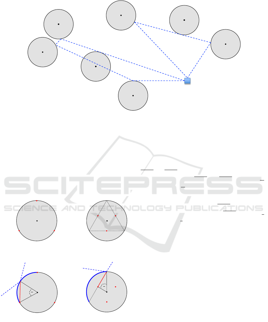
and route. In Figure 2, a solution for the mCETSP

problem is illustrated. The instance includes seven

target points

{

,...,v

}

, with their corresponding

neighborhoods represented by disks centered at these

points. The points

{

, p

,..., p

}

are the turn points

and , together with the depot 0, deﬁne the two tours:

=< 0, p

, p

,0 > and T

=< 0, p

, p

,0 >, de-

picted as dashed blue lines. In the following, we

denote a solution of mCETSP as the set of its tours

,...,T

}. Therefore, the solution of the example

is denoted by {T

2.1 The Discretized Version of mCETSP

The number of feasible solutions for the mCETSP is

inﬁnite because there are inﬁnitely many possible turn

points in each neighborhood that can be used to build

the tours. However, the number of turn points in any

feasible solution is ﬁnite (see Figure 2). To formu-

late the mCETSP as an integer linear programming

problem, each neighborhood N(v) is discretized into

a ﬁxed number k of discretization points. We denote

the set of discretization points for neighborhood N(v)

N(v), and the union of all discretization points for

the instance as

N =

v=1

N(v).

Moreover, let T (i) be a function that, given a dis-

cretization point i ∈

N, returns the target point v, if

i ∈

N(v), or the depot 0 if i is the depot. Formally,

T :

N ∪ {0} → N ∪ {0}

T (i) =

v ∈ N : i ∈

N(v), if i ̸= 0,

0, if i = 0.

The discretized version of the mCETSP corre-

sponds to a variant of the well-known Generalized

Traveling Salesman Problem (GTSP) with m vehicles

instead of a single one. For this reason, we denote the

discretized version of the mCETSP as mGTSP. To ob-

tain a feasible solution for the mGTSP, it is sufﬁcient

to ensure that at least one discretization point in each

neighborhood is visited by one of m routes.

The discretization points positioning in the neigh-

borhoods is crucial to obtain high-quality solutions

for the mCETSP. Indeed, the gap between the op-

timal solution values of mCETSP and mGTSP de-

pends on this positioning. It has been proved, in the

literature (Behdani and Smith, 2014), that the op-

timal solution of the CETSP places the turn points

of the routes on the circumferences of the neighbor-

hoods. Hence, the most intuitive strategy would in-

volve placing the discretization points along the cir-

cumferences of the neighborhoods. Such a scheme,

referred to as the Perimetral Discretization Scheme

(PD), divides each circumference C

associated with

a neighborhood N(v) into k equal circular arcs. The

discretization points are positioned at the endpoints

of these arcs. In Figure 3(a) is shown the Perime-

tral Discretization Schema with three discretization

points, d

, d

and d

, and the relative circular arcs

and

ICORES 2025 - 14th International Conference on Operations Research and Enterprise Systems

188

𝑝

<latexit sha1_base64="bNvJD3+0XyRfabhuGEoNLQMTS/Q=">AAACC3icbVC7TsNAEDyHVwivAAUFzYkEiSqyUwTKCBrKICUhUmJZ58smnHJ+6G6NiCx/Al9BCxUdouUjKPgXbOMCEqYazeze7I0bSqHRND+N0srq2vpGebOytb2zu1fdP+jrIFIcejyQgRq4TIMUPvRQoIRBqIB5roRbd3aV+bf3oLQI/C7OQ7A9NvXFRHCGqeRUj+ojhAfMH4pdGUESdx0rqTvVmtkwc9BlYhWkRgp0nOrXaBzwyAMfuWRaDy0zRDtmCgWXkFRGkYaQ8RmbwjClPvNA23Gem9DTSDMMaAiKCklzEX5vxMzTeu656aTH8E4vepn4nzeMcHJhx8IPIwSfZ0EoJORBmiuRNgN0LBQgsuxyoMKnnCmGCEpQxnkqRmlVlbQPa/H3y6TfbFitRuumWWtfFs2UyTE5IWfEIuekTa5Jh/QIJwl5Is/kxXg0Xo034/1ntGQUO4fkD4yPb+nomyM=</latexit>

<latexit sha1_base64="DHSATC82iWvrU8jeoibt7oo57Dc=">AAACC3icbVC7TsNAEDyHVwivAAUFzYkEiSqyUwTKCBrKICUhUmJZ58smnHJ+6G6NiCx/Al9BCxUdouUjKPgXbOMCEqYazeze7I0bSqHRND+N0srq2vpGebOytb2zu1fdP+jrIFIcejyQgRq4TIMUPvRQoIRBqIB5roRbd3aV+bf3oLQI/C7OQ7A9NvXFRHCGqeRUj+ojhAfMH4pdGUESd51mUneqNbNh5qDLxCpIjRToONWv0TjgkQc+csm0HlpmiHbMFAouIamMIg0h4zM2hWFKfeaBtuM8N6GnkWYY0BAUFZLmIvzeiJmn9dxz00mP4Z1e9DLxP28Y4eTCjoUfRgg+z4JQSMiDNFcibQboWChAZNnlQIVPOVMMEZSgjPNUjNKqKmkf1uLvl0m/2bBajdZNs9a+LJopk2NyQs6IRc5Jm1yTDukRThLyRJ7Ji/FovBpvxvvPaMkodg7JHxgf3+t5myQ=</latexit>

Figure 2: An example of feasible solution of mCETSP problem with seven target points and two routes.

(Carrabs et al., 2017b) proved that better results

can be achieved by positioning these discretization

points within the neighborhoods rather than on their

circumferences. This scheme, named Internal Point

Discretization Schema (IP), works as follows. Given

the number of discretization points k, IP divides C

into k equal circular arcs and places a discretization

point at the midpoint of the chord corresponding to

each arc. Figure 3(b) shows the IP schema for k = 3.

𝑝

𝑑

𝑣

𝑝

𝑑

𝑣

<latexit sha1_base64="SayPRMVZ5nQKTMgx2dfYjtbsAxQ=">AAACA3icbVC7TsNAEDzzDOFloKQ5kSBRRXaKQBlBQxkk8pDiKFpfNuGU80N360iRlZK/oIWGDtHyIUh8DE5wAQlTjWZ2tbPjx0oacpxPa219Y3Nru7BT3N3bPzi0j45bJkq0wKaIVKQ7PhhUMsQmSVLYiTVC4Cts++Obud+eoDYyCu9pGmMvgFEoh1IAZVLftotlb6hBpF4sZ+l4Vu7bJafiLMBXiZuTEsvR6Ntf3iASSYAhCQXGdF0npl4KmqRQOCt6icEYxBhG2M1oCAGaXrpIPuPniQGKeIyaS8UXIv7eSCEwZhr42WQA9GCWvbn4n9dNaHjVS2UYJ4ShmB8iqXBxyAgts0qQD6RGIpgnRy5DLkADEWrJQYhMTLKOsjrc5edXSatacWuV2l21VL/OiymwU3bGLpjLLlmd3bIGazLBJuyJPbMX69F6td6s95/RNSvfOWF/YH18Ay0Jl6M=</latexit>

⇡

𝑑

𝑣

𝑑

𝑣

𝑑

<latexit sha1_base64="2KWE0vXmPwoIzLddHXIKyLN/wH4=">AAAB9XicbVC7TsNAEDyHVwivACXNiQgpNJGNUKCMoKEMgjykxIrWl0045fzQ3RoURfkEWqjoEC3fQ8G/YBsXEJhqNLOrnR0vUtKQbX9YhaXlldW14nppY3Nre6e8u9c2YawFtkSoQt31wKCSAbZIksJupBF8T2HHm1ymfucetZFhcEvTCF0fxoEcSQGUSDdVOB6UK3bNzsD/EicnFZajOSh/9oehiH0MSCgwpufYEbkz0CSFwnmpHxuMQExgjL2EBuCjcWdZ1Dk/ig1QyCPUXCqeifhzYwa+MVPfSyZ9oDuz6KXif14vptG5O5NBFBMGIj1EUmF2yAgtkw6QD6VGIkiTI5cBF6CBCLXkIEQixkkppaQPZ/H7v6R9UnPqtfr1aaVxkTdTZAfskFWZw85Yg12xJmsxwcbskT2xZ+vBerFerbfv0YKV7+yzX7DevwAvIZHa</latexit>

(a)

<latexit sha1_base64="0PHSd84WPhkYQq9yJdEJJSRkJng=">AAAB9XicbVC7TsNAEFyHVwivACXNiQgpNJGNUKCMoKEMgjykxIrOl0045fzQ3RoURfkEWqjoEC3fQ8G/YBsXEJhqNLOrnR0vUtKQbX9YhaXlldW14nppY3Nre6e8u9c2YawFtkSoQt31uEElA2yRJIXdSCP3PYUdb3KZ+p171EaGwS1NI3R9Pg7kSApOiXRT9Y4H5YpdszOwv8TJSQVyNAflz/4wFLGPAQnFjek5dkTujGuSQuG81I8NRlxM+Bh7CQ24j8adZVHn7Cg2nEIWoWZSsUzEnxsz7hsz9b1k0ud0Zxa9VPzP68U0OndnMohiwkCkh0gqzA4ZoWXSAbKh1EjE0+TIZMAE15wItWRciESMk1JKSR/O4vd/Sfuk5tRr9evTSuMib6YIB3AIVXDgDBpwBU1ogYAxPMITPFsP1ov1ar19jxasfGcffsF6/wIwsZHb</latexit>

(b)

<latexit sha1_base64="3rc6dUe2IciS3sHw0BwXigV3pNs=">AAAB9XicbVC7TsNAEFyHVwivACXNiQgpNJGNUKCMoKEMgjykxIrOl0045fzQ3RoURfkEWqjoEC3fQ8G/YBsXEJhqNLOrnR0vUtKQbX9YhaXlldW14nppY3Nre6e8u9c2YawFtkSoQt31uEElA2yRJIXdSCP3PYUdb3KZ+p171EaGwS1NI3R9Pg7kSApOiXRTFceDcsWu2RnYX+LkpAI5moPyZ38YitjHgITixvQcOyJ3xjVJoXBe6scGIy4mfIy9hAbcR+POsqhzdhQbTiGLUDOpWCbiz40Z942Z+l4y6XO6M4teKv7n9WIanbszGUQxYSDSQyQVZoeM0DLpANlQaiTiaXJkMmCCa06EWjIuRCLGSSmlpA9n8fu/pH1Sc+q1+vVppXGRN1OEAziEKjhwBg24gia0QMAYHuEJnq0H68V6td6+RwtWvrMPv2C9fwEyQZHc</latexit>

(c)

<latexit sha1_base64="MJBkYAAZY0HwohITux054kR5PjI=">AAAB9XicbVC7TsNAEDyHVwivACXNiQgpNJGNUKCMoKEMgjykxIrWl0045fzQ3RoURfkEWqjoEC3fQ8G/YBsXEJhqNLOrnR0vUtKQbX9YhaXlldW14nppY3Nre6e8u9c2YawFtkSoQt31wKCSAbZIksJupBF8T2HHm1ymfucetZFhcEvTCF0fxoEcSQGUSDfV4fGgXLFrdgb+lzg5qbAczUH5sz8MRexjQEKBMT3HjsidgSYpFM5L/dhgBGICY+wlNAAfjTvLos75UWyAQh6h5lLxTMSfGzPwjZn6XjLpA92ZRS8V//N6MY3O3ZkMopgwEOkhkgqzQ0ZomXSAfCg1EkGaHLkMuAANRKglByESMU5KKSV9OIvf/yXtk5pTr9WvTyuNi7yZIjtgh6zKHHbGGuyKNVmLCTZmj+yJPVsP1ov1ar19jxasfGef/YL1/gUz0ZHd</latexit>

(d)

Figure 3: (a) Perimetral and (b) Internal Point Discretiza-

tion schemas for k = 3. Discretization error for (c) Perime-

tral schema and (d) Internal Point schema.

(Carrabs et al., 2017b) deﬁned the discretization

error ε

, carried out by a tour T on a neighborhood

N(v), as two times the maximum distance between

the turn point p

of T on C

and the discretization

point of

N(v) closest to p

. Figure 3(c) shows the

discretization error for the PD schema. If T inter-

sects N(v) on the circular arc

then the maxi-

mum distance occurs when p

is in the middle of this

circular arc and it is represented by the red segment

, p

(or d

, p

). From trigonometry we derive that

the length of segment d

, p

is c(d

, p

) = 2r

sin(

)

and ε

= 4r

sin(

For the IP schema, the maximum distance occurs

when p

is on an extreme of the circular arc and it is

represented by the red segment d

, p

in Figure 3(d).

By trigonometry we have that c(d

, p

) = r

sin(

)

and ε

= 2r

sin(

). Based on trigonometric consider-

ations, this implies that the discretization error carried

out by the IP schema is lower than the one carried out

by the PD schema, in particular for small values of k.

For this reason, we adopt the IP discretization schema

in this work.

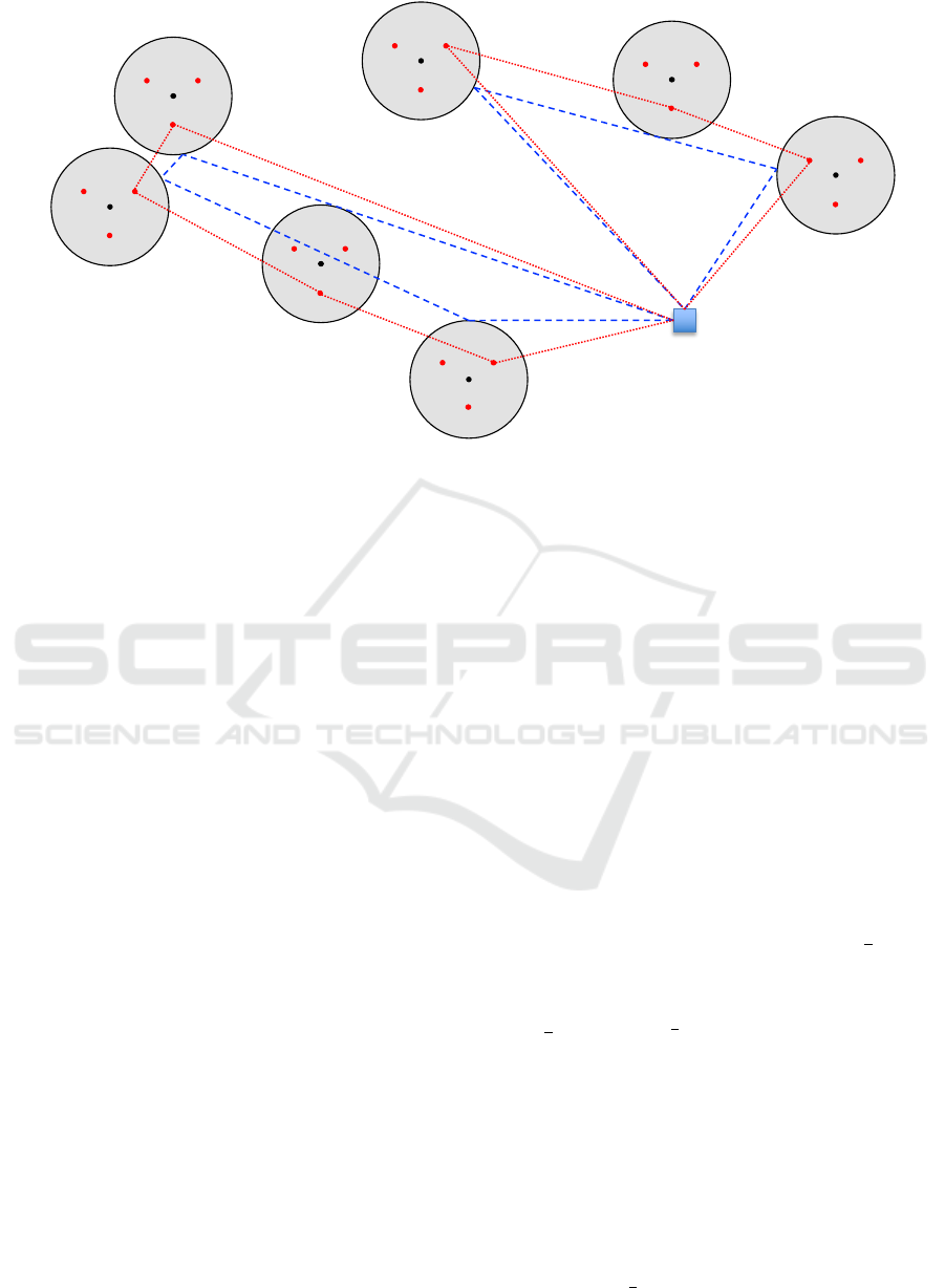
The mGTSP is deﬁned on a complete directed

graph G = (V,A), where the node set is V = {0 ∪

and the arc set is A = {(i, j) : i ∈ V, j ∈ V, i ̸= j,T (i) ̸=

T ( j)}. Figure 4 illustrates an instance of the mGTSP

with k = 3. The black points

{

,...,v

}

represent

the target points, while the red points indicate the dis-

cretization points. In this example, three discretiza-

tion points are used to discretize each neighborhood.

The depot is denoted as 0. The two tours T

and T

shown as dashed blue lines, correspond to the solu-

tion {T

} for the mCETSP, while the two tours

and

, depicted as red dotted lines, represent the so-

lution {

} for the mGTSP. Let us denote by ℓ(T )

the length of a tour T. The solution value of mCETSP

is equal to ℓ(T

) while the one of mGTSP is ℓ(

). It

is easy to see that ℓ(

) > ℓ(T

) and this occurs be-

Upper Bound Computation for the Multiple Close-Enough Traveling Salesman Problem

189

𝑝

<latexit sha1_base64="7lJSpuBLDDpG1NLiJWk5tNmz2Qs=">AAACFnicbVC5TsNAFFyHO1wGSppVEiSqyE4RKCNoKIOUQKQksp43L7DK+tDuM4cs93wCX0ELFR2ipaXgX3BMCq6pRjPvHD9W0pDjvFulufmFxaXllfLq2vrGpr21fWaiRAvsikhFuueDQSVD7JIkhb1YIwS+wnN/cjz1z69QGxmFHbqNcRjARSjHUgDlkmdXagPCGyoGpRpHWTq4liO8BEo7mZc2sqzm2VWn7hTgf4k7I1U2Q9uzPwajSCQBhiQUGNN3nZiGKWiSQmFWHiQGYxATuMB+TkMI0AzT4oSM7yUGKOIxai4VL0T83pFCYMxt4OeVAdCl+e1Nxf+8fkLjw2EqwzghDMV0EUmFxSIjtMxDQj6SGolgejlyGXIBGohQSw5C5GKSp1bO83B/f/+XnDXqbrPePG1UW0ezZJbZLquwfeayA9ZiJ6zNukywO/bAHtmTdW89Wy/W61dpyZr17LAfsN4+AXUPoFc=</latexit>

<latexit sha1_base64="M6y7ISmt7WQdEKOsrCtnNdGwwcU=">AAACFnicbVC5TsNAFFyHK4QrQEmzIkGiiuwUgTKChjJIBJCSyHrevIQV60O7z0BkuecT+ApaqOgQLS0F/4JtUgBhqtHMO8eLlDRk2x9WaW5+YXGpvFxZWV1b36hubp2bMNYCuyJUob70wKCSAXZJksLLSCP4nsIL7/o49y9uUBsZBmc0iXDgwziQIymAMsmt7tb7hHdUDEo0DtOkfyuHeAWUnKVu4qRp3a3W7IZdgM8SZ0pqbIqOW/3sD0MR+xiQUGBMz7EjGiSgSQqFaaUfG4xAXMMYexkNwEczSIoTUr4XG6CQR6i5VLwQ8WdHAr4xE9/LKn2gK/PXy8X/vF5Mo8NBIoMoJgxEvoikwmKREVpmISEfSo1EkF+OXAZcgAYi1JKDEJkYZ6lVsjycv9/PkvNmw2k1WqfNWvtomkyZ7bBdts8cdsDa7IR1WJcJds8e2RN7th6sF+vVevsuLVnTnm32C9b7F3N9oFY=</latexit>

Figure 4: Comparison between the solutions of mCETSP (in blue) and mGTSP problems (in red).

cause the use of the discretization points limits the

number of routes that the algorithms can build. For

this reason, the optimal solution value we obtain by

solving mGTSP is an upper bound to the optimal so-

lution value of mCETSP.

3 A MATHEMATICAL

FORMULATION FOR mGTSP

In this section, we present a mixed integer linear

programming formulation for the mGTSP obtained

by adapting the formulation proposed by (Bianchessi

et al., 2018) for the Team Orienteering Problem. The

formulation involves four types of variables: x

i j

, y

i j

, and z. The meaning of these variables is deﬁned

in the following.

i j

1 if the arc (i, j) is selected,

0 otherwise.

The x variables are used to describe the routes as-

signed to the drones.

1 if node i is visited,

0 otherwise.

The y variables state what are the nodes visited by

drones. These variables are necessary to assure that

each target point is covered by the routes.

i j

≥ 0

The w variables are continuous variables that state

the arrival time to the node j of a drone coming from

node i. This variable is used to calculate the length

of individual tours. Finally, variable z represents the

length of the maximum route inside the solution, and

the goal of the model is to minimize the value of this

variable.

Following the formulation proposed

by (Bianchessi et al., 2018), we introduce a sec-

ond (dummy) depot that we denote by

0. Both

depots, 0 and

0, are located in the same position

of the plane. Therefore, from now on, the graph

G = (V,A) has the node set V = {0 ∪

0 ∪

N} and the

arc set is A = {(i, j ) : i ∈ V, j ∈ V,i ̸= j, T (i) ̸= T ( j)}

with T (

0) =

In order to present our mathematical formulation

for mGTSP, we need the following notation.

• T

max

: Maximum length of a route;

• m: Number of routes;

• t

i j

: Travel time from node i to j, where t

= 0 and

= 0;

• t

i j

= t

i j

;

• T

max

= T

max

−t

;

• δ

(S) = {(i, j) ∈ A : i ∈ S, j /∈ S}: Set of arcs leav-

ing the set S, with S ⊆

N ∪ {0,

0};

• δ

−

(S) = {(i, j) ∈ A : i /∈ S , j ∈ S}: Set of arcs en-

tering the set S, with S ⊆

N ∪ {0,

0}.

The mathematical formulation of the mGTSP is the

following:

(MIP) min z (1)

∑

j∈

0 j

∑

i∈

= m (2)

ICORES 2025 - 14th International Conference on Operations Research and Enterprise Systems

190

∑

( j,i)∈δ

−

(i)

∑

(i, j)∈δ

(i)

i j

= y

i ∈

N (3)

∑

i∈

N(v)

= 1 v ∈ N (4)

0 j

= t

0 j

j ∈

N (5)

∑

(i, j)∈δ

(i)

i j

−

∑

( j,i)∈δ

−

(i)

∑

(i, j)∈δ

(i)

i j

i ∈

(6)

i j

≤ T

max

i j

(i, j ) ∈ A \ {(0, 0)} (7)

i j

≥ t

i j

(i, j ) ∈ A \ {(0, 0)} (8)

z ≥ w

i ∈

N (9)

∈ {0,1} i ∈

N (10)

i j

≥ 0 i, j ∈

N (11)

i j

∈ {0,1} (i, j) ∈ A \ {(0, 0)} (12)

• The objective function (1) aims to minimize the

variable z that represents the length of the maxi-

mum route inside the solution;

• Constraint (2) impose that exactly m routes have

to start from the depot 0 and end into the depot

This assure that all the required routes are deﬁned

and that each route starts and ends into the depot;

• Constraint (3) assure that a discretization node i

is entered and leaved exactly once if it is visited

(i.e., if y

= 1);

• Constraint (4) ensures that exactly one discretiza-

tion point in the neighborhood

N(v) of each target

point v is visited. Since in our problem, we use the

Euclidean distances, the triangle inequality holds.

This means that always exists an optimal solution

to the problem that visits one point for each neigh-

borhood.

• Constraint (5) assigns to variable w

0 j

the arrival

time of a route into node j coming directly from

depot 0.

• Constraint (6) ensures that the w

i j

variables are

correctly updated according to the arcs selected

(i.e. x

i j

= 1).

• Constraint (7) sets an upper limit on the duration

of each route.

• Constraint (8) sets a lower bound on the values

of w

i j

, ensuring w

i j

represents the arrival time at

node j if x

i j

= 1, otherwise w

i j

= 0.

• Constraint (9) ensures that the variable z equals

the length of the maximum route.

• Finally, (10)-(12) are variables deﬁnition con-

straints.

To enhance the strength of the model, an addi-

tional constraint can be introduced to limit the overall

duration of all routes combined:

∑

(i, j)∈A\(0,0)

i j

≤ mT

max

(13)

In our model, the T

max

parameter plays a funda-

mental role in determining the feasibility of solutions,

as it represents an upper limit on the maximum route

duration for each drone. In order to compute an upper

limit of the optimal solution value, we take a feasi-

ble solution T of the CETSP and add to its value c(T )

the discretization error ε

= 2r

sin





carried out for

each neighborhood

N(v) inside a route. Formally:

max

c(T ) +

∑

v∈N

•

(14)

It is worth noting that the ε

value depends on

the r

value and, in general, the neighborhoods could

have different radii. Since T

max

is used as a bigM

value inside the model, we would to minimize its

value to improve the performance of the model. To

this end, we observe that each of the m routes must

contain at least one discretization point. This means

that, the maximum number of discretization points

inside a route for mGTSP, is equal to |N| − (m − 1).

Therefore, the total discretization error, carried out in

any route, can be computed by adding the |N| − (m −

1) largest ε

values. By denoting with N

the set of

|N|−(m − 1) largest ε

values, we update the formula

to compute T

max

as follow:

max

c(T ) +

∑

v∈N

•

(15)

3.1 Graph Reduction Algorithm (GRA)

In order to speed up the computation of the upper

bound, the graph reduction algorithm (GRA) pro-

posed in (Carrabs et al., 2017b), is applied on G =

(V,A) to remove nodes and arcs that will not con-

tribute to the optimal solution. Furthermore, we pro-

vide a proof of correctenss of GRA in the context of

mGTSP, as GRA was originally proposed for a dis-

cretized version of CETSP while in our case we have

m routes and a different objective function.

GRA works as follows. Let v be a target point

and let i ∈ V and j ∈ V be two points such that

T (i) ̸= T ( j) ̸= v (see Figure 5). According to the

Euclidean distance, the algorithm computes the short-

est path from i to j passing through r, for each point

Upper Bound Computation for the Multiple Close-Enough Traveling Salesman Problem

191

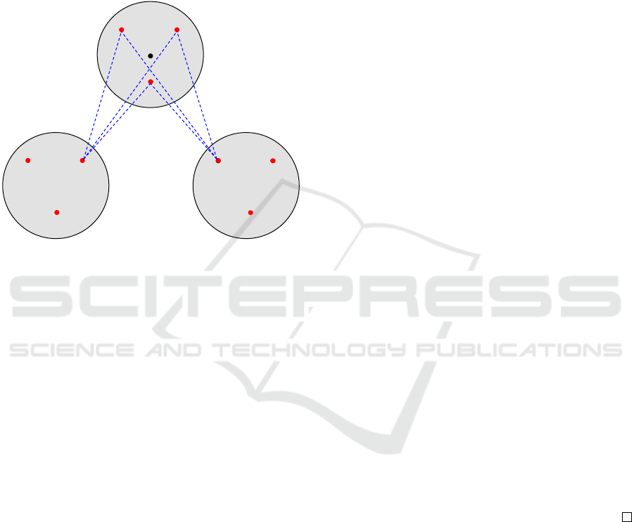
r ∈

N(v). Notice that these shortest paths are always

composed of two edges (i,r) and (r, j). Among all

the shortest paths computed, the algorithm saves the

shortest one, which we denote from now on as S

(i,v, j)

and it marks as necessary its two edges and the point

N(v) belong to it. This computation is repeated

for each target point v ∈ N and for each pair of points

i ∈ V and j ∈ V with T (i) ̸= T ( j ) ̸= v.

<latexit sha1_base64="vooPYmnqnlyVjVWccOWJVT5nwWw=">AAAB9XicbVC7TsNAEDyHVwivACXNiQSJKrJTBMoIGsogyENKrOh82YRTzmfrbh0UWfkEWqjoEC3fQ8G/YBsXkDDVaGZXOzteKIVB2/60CmvrG5tbxe3Szu7e/kH58KhjgkhzaPNABrrnMQNSKGijQAm9UAPzPQldb3qd+t0ZaCMCdY/zEFyfTZQYC84wke6qs+qwXLFrdga6SpycVEiO1rD8NRgFPPJBIZfMmL5jh+jGTKPgEhalQWQgZHzKJtBPqGI+GDfOoi7oWWQYBjQETYWkmQi/N2LmGzP3vWTSZ/hglr1U/M/rRzi+dGOhwghB8fQQCgnZIcO1SDoAOhIaEFmaHKhQlDPNEEELyjhPxCgppZT04Sx/v0o69ZrTqDVu65XmVd5MkZyQU3JOHHJBmuSGtEibcDIhT+SZvFiP1qv1Zr3/jBasfOeY/IH18Q1BQpHk</latexit>

<latexit sha1_base64="dOvC3Et+WZHqNOlAoPO+JEP1dZg=">AAAB9XicbVC7TsNAEDzzDOEVoKQ5kSBRRXaKQBlBQxkEeUiJFa0vm3DK+aG7NSiK8gm0UNEhWr6Hgn/BNi4gYarRzK52drxISUO2/WmtrK6tb2wWtorbO7t7+6WDw7YJYy2wJUIV6q4HBpUMsEWSFHYjjeB7Cjve5Cr1Ow+ojQyDO5pG6PowDuRICqBEuq3oyqBUtqt2Br5MnJyUWY7moPTVH4Yi9jEgocCYnmNH5M5AkxQK58V+bDACMYEx9hIagI/GnWVR5/w0NkAhj1BzqXgm4u+NGfjGTH0vmfSB7s2il4r/eb2YRhfuTAZRTBiI9BBJhdkhI7RMOkA+lBqJIE2OXAZcgAYi1JKDEIkYJ6UUkz6cxe+XSbtWderV+k2t3LjMmymwY3bCzpjDzlmDXbMmazHBxuyJPbMX69F6td6s95/RFSvfOWJ/YH18AzsCkeA=</latexit>

<latexit sha1_base64="pQn+2SMFLdhIEQgukFWgvrDgS78=">AAAB9XicbVC7TsNAEDzzDOEVoKQ5kSBRRXaKQBlBQxkEeUiJFa0vm3DK+aG7NSiK8gm0UNEhWr6Hgn/BNi4gYarRzK52drxISUO2/WmtrK6tb2wWtorbO7t7+6WDw7YJYy2wJUIV6q4HBpUMsEWSFHYjjeB7Cjve5Cr1Ow+ojQyDO5pG6PowDuRICqBEuq3IyqBUtqt2Br5MnJyUWY7moPTVH4Yi9jEgocCYnmNH5M5AkxQK58V+bDACMYEx9hIagI/GnWVR5/w0NkAhj1BzqXgm4u+NGfjGTH0vmfSB7s2il4r/eb2YRhfuTAZRTBiI9BBJhdkhI7RMOkA+lBqJIE2OXAZcgAYi1JKDEIkYJ6UUkz6cxe+XSbtWderV+k2t3LjMmymwY3bCzpjDzlmDXbMmazHBxuyJPbMX69F6td6s95/RFSvfOWJ/YH18Ayzykdc=</latexit>

<latexit sha1_base64="qJpX/pVz/5viYKzZDsp1IU8goLs=">AAAB9XicbVC7TsNAEDyHVwivACXNiQSJKrJTBMoIGsogyENKrOh82YQj57N1twZFVj6BFio6RMv3UPAv2MYFJEw1mtnVzo4XSmHQtj+twsrq2vpGcbO0tb2zu1feP+iYINIc2jyQge55zIAUCtooUEIv1MB8T0LXm16mfvcBtBGBusVZCK7PJkqMBWeYSDfV++qwXLFrdga6TJycVEiO1rD8NRgFPPJBIZfMmL5jh+jGTKPgEualQWQgZHzKJtBPqGI+GDfOos7pSWQYBjQETYWkmQi/N2LmGzPzvWTSZ3hnFr1U/M/rRzg+d2OhwghB8fQQCgnZIcO1SDoAOhIaEFmaHKhQlDPNEEELyjhPxCgppZT04Sx+v0w69ZrTqDWu65XmRd5MkRyRY3JKHHJGmuSKtEibcDIhT+SZvFiP1qv1Zr3/jBasfOeQ/IH18Q0ugpHY</latexit>

<latexit sha1_base64="8hnerFaxKwdSmNXqiWVuWoarfZo=">AAAB93icbVC7TsNAEDyHVwivACXNiQRBFdkpAmUEDWWQcBIpsaLzZRNOOZ+tuzVSZOUbaKGiQ7R8DgX/gm1cQMJUo5ld7ez4kRQGbfvTKq2tb2xulbcrO7t7+wfVw6OuCWPNweWhDHXfZwakUOCiQAn9SAMLfAk9f3aT+b1H0EaE6h7nEXgBmyoxEZxhKrl1fV6vjKo1u2HnoKvEKUiNFOiMql/DccjjABRyyYwZOHaEXsI0Ci5hURnGBiLGZ2wKg5QqFoDxkjzsgp7FhmFII9BUSJqL8HsjYYEx88BPJwOGD2bZy8T/vEGMkysvESqKERTPDqGQkB8yXIu0BaBjoQGRZcmBCkU50wwRtKCM81SM01qyPpzl71dJt9lwWo3WXbPWvi6aKZMTckouiEMuSZvckg5xCSeCPJFn8mLNrVfrzXr/GS1Zxc4x+QPr4xvS55Il</latexit>

<latexit sha1_base64="za5Tqt2X8dBxoH2JAOy2mNQ6BRM=">AAAB+HicbVC7TsNAEDzzDOEVoKQ5kaBQRXaKQBlBQxkk8pASKzpfNuHI+WzdrZGClX+ghYoO0fI3FPwLtnEBCVONZna1s+OFUhi07U9rZXVtfWOzsFXc3tnd2y8dHHZMEGkObR7IQPc8ZkAKBW0UKKEXamC+J6HrTa9Sv/sA2ohA3eIsBNdnEyXGgjNMpE5FV6uV4rBUtmt2BrpMnJyUSY7WsPQ1GAU88kEhl8yYvmOH6MZMo+AS5sVBZCBkfMom0E+oYj4YN87SzulpZBgGNARNhaSZCL83YuYbM/O9ZNJneGcWvVT8z+tHOL5wY6HCCEHx9BAKCdkhw7VIagA6EhoQWZocqFCUM80QQQvKOE/EKOkl7cNZ/H6ZdOo1p1Fr3NTLzcu8mQI5JifkjDjknDTJNWmRNuHknjyRZ/JiPVqv1pv1/jO6YuU7R+QPrI9vNcGSVg==</latexit>

Figure 5: Example of shortest paths computed using Graph

Reduction Algorithm.

At the end of the computation, GRA removes all

the edges and nodes not marked, that is, the ones

that do not belong to any shortest path S

(i,v, j)

. No-

tice that the depots are marked by default because

they are necessary for the construction of the routes.

In the following, with a little abuse of notation, we

use the ℓ function to denote the length of paths too.

Let us consider the example depicted in Figura 5.

GRA computes the three shortest paths < i,r, j >,

< i,r

′

, j > and < i,r

′′

, j >. Since, among these three

paths, the shortest one is < i,r, j >, the algorithm

marks the arcs (i,r), (r, j) and the node r. Moreover,

(i,v, j)

=< i,r, j >. Theorem 1 proves that by apply-

ing GRA to the graph, the optimal solution of mGTSP

does not change.

Theorem 1. Let S = ∪

i∈V, j∈V,v∈N,T (i)̸=T ( j)̸=v

(i,v, j)

the set of shortest paths saved by GRA algorithm.

Given a target point v ∈ N, any edge (x,y) ∈ A, in-

cident to

N(v) and not belonging to any shortest path

in S, either does not belong to the optimal solution

{

∗

,...,

∗

} or there is an alternative optimal so-

lution without this arc.

Proof. Let us suppose that the arc (x,y) belongs to a

tour

∗

of the optimal solution, with x ∈

N(v), and let

q be the point that coming just before x in

∗

. There

are the following two cases to consider:

∗

is the longest tour of the optimal solution and

the other tours are shorter than it.

In this case we have that ℓ(

∗

) > ℓ(

∗

), with p =

{1,...,m} \ {h}, and the optimal solution value is

equal to ℓ(

∗

). We have to consider the following

subcases:

• ℓ(< q, x, y >) > ℓ(S

(q,v,y)

Since the arc (x,y) do not belong to S

(q,v,y)

than there exists another discretization point

r ∈

N(v) such that the path < q,r,y > is shorter

than < q,x, y >. This means that, by replac-

ing < q,x,y > with < q,r,y > in

∗

, we obtain

a new shortest tour

∗

′

and then a new solution

{

∗

,...,

∗

′

,...,

∗

} better than the optimal

one. A contradiction.

• ℓ(< q, x, y >) = ℓ(S

(q,v,y)

This situation occurs when S

(q,v,y)

can be build

by using more different discretization points

N(v). Let us suppose that r ∈

N(v) is an-

other discretization point of

N(v) such that ℓ(<

q,x,y >) = ℓ(< q,r, y >). This means that, by

replacing < q,x,y > with < q,r,y > in

∗

, we

obtain another tour

∗

′

with ℓ(

∗

) = ℓ(

∗

′

) and

then {

∗

,...,

∗

′

,...,

∗

} is an alternative

optimal solution that does not contain the arc

(x,y).

∗

is the longest tour of the optimal solution with

p ̸= h.

In this case we have that ℓ(

∗

) ≤ ℓ(

∗

). More-

over, since (x,y) does not belonging to any short-

est path in S then ℓ(< q,x,y >) ≥ ℓ(S

(q,v,y)

). As

a consequence, by replacing < q, x, y > with <

q,r, y > in

∗

, we obtain a new tour

∗

′

with

ℓ(

∗

′

) ≤ ℓ(

∗

). This means that the solution

{

∗

,...,

∗

′

,...,

∗

} have the same cost of the

optimal one and then it is an alternative optimal

solution that does not contain the arc (x,y).

4 COMPUTATIONAL TESTS

In this section, we describe the results of our MIP

model for mGTSP obtained during our computational

test phase. The model was coded in C++ and solved

using the IBM ILOG CPLEX 22.1.1 solver. A time

limit of one hour, a thread limit of 4, a memory limit

of 16 GB were imposed. Moreover, the relative and

absolute MIP gap tolerance are set to 1e-7. All re-

maining CPLEX parameters were left to their default

value. All tests were performed on an OSX platform

ICORES 2025 - 14th International Conference on Operations Research and Enterprise Systems

192

(iMac 2020), running on an Intel Core i9-10910 pro-

cessor clocked at 3.6 GHz with 64 GB of RAM.

The computational tests are carried out on 360 in-

stances having 6, 8, 10 and 12 target points and three

radius values: 0.25, 0.50, and 1.00. There are 30 in-

stances for each combination of the number of tar-

get points and the radius values. This is a subset of

the instances proposed by (Behdani and Smith, 2014)

for the CETSP problem. For this set of instances, the

optimal values of the CETSP solutions are available.

So, since it is the smallest possible value as c(T ), we

use it to calculate T

max

as described in Section 2.

It is worth noting that in CETSP all the neighbor-

hoods must be covered by a single route whereas in

mGTSP the same task is carried out using m routes.

Therefore, it could be natural to think that the opti-

mal solution value of CETSP is an upper bound of the

optimal solution value of mGTSP but it’s not always

like this. Indeed, the use of the discretization points,

in mGTSP, generates a discretization error, for each

neighborhood, that must be added to the cost of the

routes and then the optimal solution value of CETSP

may be lower than the one of mGTSP.

Due to the complexity of mGTSP and to limit

the size of the instances, we use three discretization

points (that is k = 3) for each neighborhood. This

means that for a problem with 10 target nodes, the

model will solve an instance with 3 × 10 + 2 = 32

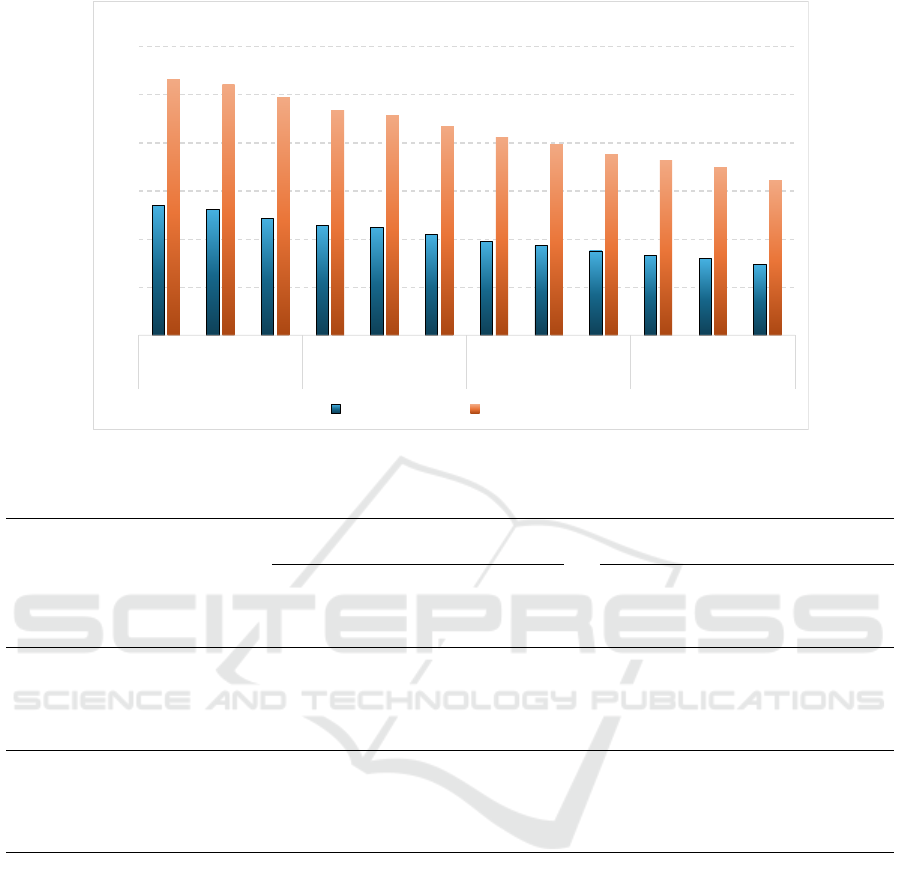
nodes. We start our computational study by evalu-

ating the effectiveness of the GRA algorithm. In Fig-

ure 6 the percentages of nodes and arcs removed by

the GRA algorithm are shown. The four scenarios,

with 6, 8, 10 and 12 target points and radii 0.25, 0.5

and 1, are reported on the x-axis, each one composed

of thirty instances. These results highlight the effec-

tiveness of GRA which removes always more than

14% of nodes and 32% of edges. In more detail, the

percentage of nodes removed ranges from 14.6%, in

the scenario with 12 target points and a radius equal

to 1, up to 27%, in the scenario with 6 target points

and a radius equal to 0.25. A similar trend is ob-

served for the arcs too but with higher percentage val-

ues. Indeed, the percentage of arcs removed ranges

from 32.4%, in the scenario with 12 target points and

a radius equal to 1, to 53.3%, in the scenario with

6 target points and a radius equal to 0.25. Figure 6

shows a clear trend in which GRA is more effective

in the instances with the smaller radius and smallest

number of targets in both the removal of nodes and

arcs. Since the new graph produced by GRA contains

a much smaller number of nodes and edges, the MIP

model requires less computational time to ﬁnd the op-

timal solution.

In Table 1 we evaluate the performance of the MIP

model. Each row of the table contains values com-

puted on a test scenario composed of 30 instances.

The ﬁrst four columns of the table report the char-

acteristics of the instances that is: the length of the

radius (Radius), the number of target points (Target),

the number of nodes (Nodes) and arcs (Arcs). The

next ﬁve columns report, for m = 2, the average ob-

jective value (Obj), the average computational time

(Time), in seconds, the number of optimal (#Opt) and

feasible (#Feas) solutions found by model and the av-

erage of the optimality gap (Gap%). The last ﬁve

columns report the same information but with m = 3.

Table 1 shows that, for m = 2, MIP ﬁnds the opti-

mal solution on 291 out of 360 instances within the

time limit of 1 hour. In particular, all the small in-

stances with 20 and 26 nodes are solved optimally in

less than 40 seconds whatever is the radius value. On

the larger instances, with 32 and 38 nodes, MIP ﬁnds

the optimal solution on 111 out of 180 instances. The

optimality gap percentage is at most 2.19% for the

instances with 32 nodes and lower than 9% for the in-

stances with 38 nodes. These optimality gaps show

that, in the largest instances with 38 nodes, the in-

cumbent solution found by the model, is not too far

from the optimal one when two drones are used. Fi-

nally, the average computational time is lower than

2450 seconds. The performance of the model wors-

ens when we increase the number of drones used to

3. Indeed, MIP ﬁnds the optimal solution on 230 out

of 360 instances for m = 3. In particular, all the small

instances with 20 and 26 nodes are solved to optimal-

ity but the computational time grows up to 73 sec-

onds. On the larger instances, with 32 and 38 nodes,

MIP ﬁnds the optimal solution on 50 out of 180 in-

stances and the optimality gap percentage reaches ap-

proximately 8% for the instances with 32 nodes, and

21% for the instances with 38 nodes. Finally, the av-

erage computational time grows up to 3290 seconds.

These results highlight that the number of routes used

impacts both the quality of the ﬁnal solution found

by the model and the computational time required to

obtain it.

5 CONCLUSION

In this article, we studied the Multiple Close-Enough

Traveling Salesman Problem (mCETSP), a variant

of the Close-Enough Traveling Salesman Problem

(CETSP), where multiple vehicles are used to visit a

given number of target points. Due to the complexity

of the problem we adopted a discretization schema

that reduced mCETSP to the Multiple Generalized

Traveling Salesman Problem (mGTSP). For this dis-

Upper Bound Computation for the Multiple Close-Enough Traveling Salesman Problem

193

10%

20%

30%

40%

50%

60%

0.25 0.50 1.00 0.25 0.50 1.00 0.25 0.50 1.00 0.25 0.50 1.00

6 8 10 12

Reduction Percentage

Node Reduction Arc Reduction

Figure 6: Percentage of nodes and arcs removed by GRA algorithm.

Table 1: Test Results of the MIP model.

2 vehicles 3 vehicles

Radius Target Nodes Arcs Obj Time #Opt #Feas Gap% Obj Time #Opt #Feas Gap%

0.25

6 20 306 22.85 0.30 30 0 0.00% 21.37 0.40 30 0 0.00%

8 26 552 25.52 18.94 30 0 0.00% 23.53 40.60 30 0 0.00%

10 32 870 26.80 859.84 26 4 1.04% 24.57 2162.57 15 15 6.79%

12 38 1260 28.70 2353.16 13 17 6.92% 26.20 3182.36 3 27 19.23%

0.50

6 20 306 22.53 0.40 30 0 0.00% 21.14 0.45 30 0 0.00%

8 26 552 25.17 24.80 30 0 0.00% 23.30 46.33 30 0 0.00%

10 32 870 26.38 978.08 24 6 1.54% 24.28 2264.88 14 16 7.65%

12 38 1260 28.24 2442.80 13 17 7.47% 25.90 3089.85 3 27 19.95%

1.00

6 20 306 21.93 0.65 30 0 0.00% 20.69 0.56 30 0 0.00%

8 26 552 24.53 39.83 30 0 0.00% 22.84 72.76 30 0 0.00%

10 32 870 25.60 1123.15 23 7 2.19% 23.76 2438.22 13 17 8.27%

12 38 1260 27.41 2441.69 12 18 8.88% 25.32 3288.45 2 28 21.68%

cretized version, we proposed a mixed integer lin-

ear Programming formulation which provides an up-

per bound for the optimal solution value of mCETSP,

given the discretization error introduced. Addition-

ally, we applied a graph reduction algorithm (GRA)

to reduce the problem size, and we provided a proof

of its correctness as the algorithm was originally pro-

posed for a discretized version of CETSP. The compu-

tation tests performed on benchmark instances of the

CETSP highlights i) the effectiveness of GRA in sig-

niﬁcantly reducing the number of nodes and arcs, and

ii) the impact of the number of routes on the perfor-

mance on the mathematical model. A potential direc-

tion for future research is to improve the mathematical

model and develop effective metaheuristics.

ACKNOWLEDGEMENTS

We acknowledge ﬁnancial support under the National

Recovery and Resilience Plan (NRRP), Mission 4,

Component 2, Investment 1.1, Call for tender No.

1409 published on 14.9.2022 by the Italian Ministry

of University and Research (MUR), funded by the

European Union – NextGenerationEU– Project Title

“Smart Agriculture by Collaborative Robots Swarm”

– CUP P2022E38SJ - Grant Assignment Decree No.

1379 adopted on 01.09.2023 by the Italian Ministry

of Ministry of University and Research (MUR).

ICORES 2025 - 14th International Conference on Operations Research and Enterprise Systems

194

REFERENCES

Behdani, B. and Smith, J. C. (2014). An integer-

programming-based approach to the close-enough

traveling salesman problem. INFORMS Journal on

Computing, 26(3):415 – 432.

Bianchessi, N., Mansini, R., and Speranza, M. G. (2018).

A branch-and-cut algorithm for the team orienteering

problem. International Transactions in Operational

Research, 25(2):627–635.

Cariou, C., Moiroux-Arvis, L., Bendali, F., and Mailfert,

J. (2024). Optimal route planning of an unmanned

aerial vehicle for data collection of agricultural sen-

sors. In IEEE INFOCOM 2024-IEEE Conference on

Computer Communications Workshops (INFOCOM

WKSHPS), pages 1–6. IEEE.

Carrabs, F., Cerrone, C., Cerulli, R., and D’Ambrosio, C.

(2017a). Improved upper and lower bounds for the

close enough traveling salesman problem. In Au, M.

H. A., Castiglione, A., Choo, K.-K. R., Palmieri, F.,

and Li, K.-C., editors, Green, Pervasive, and Cloud

Computing, pages 165–177, Cham. Springer Interna-

tional Publishing.

Carrabs, F., Cerrone, C., Cerulli, R., and Gaudioso, M.

(2017b). A novel discretization scheme for the close

enough traveling salesman problem. Computers and

Operations Research, 78:163 – 171.

Carrabs, F., Cerrone, C., Cerulli, R., and Golden, B. (2020).

An adaptive heuristic approach to compute upper and

lower bounds for the close-enough traveling sales-

man problem. INFORMS Journal on Computing,

32(4):1030–1048.

Coutinho, W. P., Nascimento, R. Q. d., Pessoa, A. A., and

Subramanian, A. (2016). A branch-and-bound algo-

rithm for the close-enough traveling salesman prob-

lem. INFORMS Journal on Computing, 28(4):752–

765.

Dolias, G., Benos, L., and Bochtis, D. (2022). On the rout-

ing of unmanned aerial vehicles (uavs) in precision

farming sampling missions. In Information and Com-

munication Technologies for Agriculture—Theme III:

Decision, pages 95–124. Springer.

Dong, J., Yang, N., and Chen, M. (2007). Heuristic ap-

proaches for a tsp variant: The automatic meter read-

ing shortest tour problem. Extending the horizons:

Advances in computing, optimization, and decision

technologies, pages 145–163.

Gulczynski, D. J., Heath, J. W., and Price, C. C. (2006).

The close enough traveling salesman problem: A dis-

cussion of several heuristics. Perspectives in Opera-

tions Research: Papers in Honor of Saul Gass’ 80 th

Birthday, pages 271–283.

Lei, Z. and Hao, J.-K. (2024). An effective memetic algo-

rithm for the close-enough traveling salesman prob-

lem. Applied Soft Computing, 153:111266.

Mennell, W., Golden, B., and Wasil, E. (2011). A steiner-

zone heuristic for solving the close-enough traveling

salesman problem. In 2th INFORMS computing soci-

ety conference: operations research, computing, and

homeland defense.

Mennell, W. K. (2009). Heuristics for solving three routing

problems: Close-enough traveling salesman problem,

close-enough vehicle routing problem, and sequence-

dependent team orienteering problem. University of

Maryland, College Park.

Wang, X., Golden, B., and Wasil, E. (2019). A Steiner zone

variable neighborhood search heuristic for the close-

enough traveling salesman problem. Computers &

Operations Research, 101(1):200–219.

Yang, Z., Xiao, M.-Q., Ge, Y.-W., Feng, D.-L., Zhang, L.,

Song, H.-F., and Tang, X.-L. (2018). A double-loop

hybrid algorithm for the traveling salesman problem

with arbitrary neighbourhoods. European Journal of

Operational Research, 265(1):65–80.

Yuan, B., Orlowska, M., and Sadiq, S. (2007). On the

optimal robot routing problem in wireless sensor net-

works. IEEE transactions on knowledge and data en-

gineering, 19(9):1252–1261.

Upper Bound Computation for the Multiple Close-Enough Traveling Salesman Problem

195