Layerwise Image Vectorization via Bayesain-Optimized Contour

Ghfran Jabour

, Sergey Muravyov

and Valeria Eﬁmova

ITMO University, Kronverksky Pr. 49, bldg. A, St. Petersburg, 197101, Russia

ﬁ

Keywords:

Image Vectorization, Contour-Based Initialization, Bayesian Optimization, Scalable Vector Graphics,

Computational Efﬁciency, Reconstruction Fidelity, Path Optimization, Digital Content Creation, Semantic

Simpliﬁcation, Superpixel-Based Vectorization.

Abstract:

This work presents a novel method LIVBOC for complex image vectorization that addresses key challenges in

path initialization, color assignment, and optimization. Unlike existing approaches such as LIVE, our method

generates Bayesian-optimized contour for path initialization, which is then optimized using a customized loss

function to align it better with the target shape in the image. In our method, adaptive selection of points and

parameters for efﬁcient and accurate vectorization is enabled to reduce unnecessary iterations and computa-

tional overhead. LIVBOC achieves superior reconstruction ﬁdelity with fewer paths, and that is due to the

path initialization technique, which initializes paths as contours that approximate target shapes in the image,

reducing redundancy in points and paths. The experimental evaluation indicates that LIVBOC outperforms

LIVE in all key metrics, including a signiﬁcant reduction in L

loss, processing time, and ﬁle size. LIVBOC

achieves comparable results with just 100 iterations, compared to LIVE’s 500 iterations, while preserving ﬁner

details and generating smoother, more coherent paths. These improvements make LIVBOC more suitable for

applications that require scalable, compact vector graphics, and computational efﬁciency. By achieving both

accuracy and efﬁciency, LIVBOC offers a new robust alternative for image vectorization tasks. The LIVBOC

code is available at https://github.com/CTLab-ITMO/LIVBOC.

1 INTRODUCTION

Image vectorization, the process of converting raster

images into scalable vector graphics (SVG), has be-

come an essential tool in various ﬁelds, including

graphic design, web development, and scientiﬁc vi-

sualization. Vector graphics offer distinct advantages

over raster images, such as inﬁnite scalability, smaller

ﬁle sizes, and efﬁcient editing capabilities. Despite

the importance of vector graphics, this process comes

with multiple challenges. Obtaining high-quality vec-

torization, especially for complex images with impor-

tant details, is not an easy task (Dziuba et al., 2023),

as we will need to trade off many metrics listed above.

Image vectorization methods must balance the ﬁdelity

of reconstruction, computational efﬁciency, and com-

pactness while preserving the key features of the input

image.

Many traditional vectorization methods often use

ﬁxed strategies for path initialization and parame-

https://orcid.org/0009-0003-8092-9804

https://orcid.org/0000-0002-4251-1744

https://orcid.org/0000-0002-5309-2207

Input Paths Initialized Paths Optimized

Figure 1: Example showing the output of each stage of

the LIVBOC method (path initialization and path optimiza-

tion).

ter settings, which limit their ability to adapt to di-

verse image contents. As an example, SAMVG (Zhu

et al., 2023) utilizes segmentation models for vector-

ization, but highly depends on the quality of segmen-

tation maps, which may struggle with overlapping

objects. Another example is SuperSVG (Hu et al.,

2024), which simpliﬁes vectorization using superpix-

els but may sacriﬁce ﬁne details in highly textured ar-

eas. Recent advances, such as LIVSS (Wang et al.,

Jabour, G., Muravyov, S. and Eﬁmova, V.

Layerwise Image Vectorization via Bayesain-Optimized Contour.

DOI: 10.5220/0013381000003912

Paper published under CC license (CC BY-NC-ND 4.0)

In Proceedings of the 20th International Joint Conference on Computer Vision, Imaging and Computer Graphics Theory and Applications (VISIGRAPP 2025) - Volume 3: VISAPP, pages

831-838

ISBN: 978-989-758-728-3; ISSN: 2184-4321

831

2024), incorporate semantic segmentation to priori-

tize meaningful regions but are computationally in-

tensive due to their iterative processing.

To achieve a high-quality low-sized SVGs, we

propose LIVBOC (Layer-wise Image Vectorization

with Bayesian-Optimized Contours), an image vec-

torization method of two main stages, a Bayesian-

optimized contour-based path initialization stage and

a path optimization stage. Contour-based techniques

have been shown to be effective in capturing shape

boundaries while minimizing redundancy (Arbel

aez

et al., 2011; Polewski et al., 2024). Furthermore,

Bayesian optimization (Frazier, 2018; Snoek et al.,

2012) have found widespread use in machine learning

for hyperparameter optimization. Building on those

two well-established techniques, the ﬁrst stage of our

method utilizes the Bayesian optimization algorithm

to determine the optimal values for the parameters

used in identifying the optimal contour used in path

initialization. This stage gives the method the ability

to adapt to the complexity and variations of colors in

the input image. In the second stage, after path initial-

ization, we optimize the initialized path with a cus-

tom loss function composed of three loss functions:

the reconstruction loss to preserve information and

guarantee a correct direction of the path during the

optimization process, the Laplacian smoothness loss

based on (Sorkine et al., 2004) to ensure smoothness

of paths, and the overlap loss to prevent shapes from

overlapping with other correct shapes. With these two

stages, LIVBOC ensures not only achieving superior

reconstruction ﬁdelity but also reducing the number

of required paths and computational time. Unlike pre-

vious methods, which often require a ﬁxed number of

iterations for convergence, LIVBOC achieves high-

quality results with few iterations by integrating ro-

bust initialization with efﬁcient optimization. Thus,

our method ﬁts for applications demanding scalable

and high-ﬁdelity vector graphics, such as web graph-

ics, logo design, and digital content creation.

In our experiments, we compare our LIVBOC

method with LIVE (Ma et al., 2022) and demonstrate

LIVBOC strength. Through a multi-faceted compari-

son, we highlight the efﬁciency of our method in gen-

erating high-quality vector image with optimal primi-

tives (optimal SVG ﬁle size).

Key contributions of our paper are as follows:

• We propose LIVBOC, a novel image vectoriza-

tion method that generates minimized SVG ﬁles

by using an adaptive number of points for differ-

ent paths.

• The resulting vector primitives are optimal or

near-optimal, allowing the user to better manip-

ulate the vectors.

• The proposed LIVBOC method is 3-5 times faster

than current state-of-the-art machine learning-

based vectorization.

2 RELATED WORK

2.1 Layered Image Vectorization via

Semantic Simpliﬁcation (LIVSS)

The LIVSS method (Wang et al., 2024) is a novel ap-

proach to image vectorization that uses semantic in-

formation to guide the vectorization process. In this

method, Score Distillation Sampling (SDS) and se-

mantic segmentation are calculated to iteratively sim-

plify an input image while preserving essential fea-

tures. By doing that, LIVSS creates a series of sim-

pliﬁed layers, each of these layers contains varying

levels of detail. Then these layers are optimized to

create a high-quality vector representations with ad-

justable levels of ﬁdelity.

The main strength of LIVSS is the ability to bal-

ance detail preservation and vectorization compact-

ness. Using semantic segmentation, the method pri-

oritizes meaningful regions ﬁrst, with the possibility

of ignoring redundant details in the background. This

technique makes LIVSS effective for applications of

vectorizing images containing semantic meaningful

shapes.

Despite that, the performance of LIVSS is highly

dependent on the quality of its semantic segmentation.

Therefore, if segmentation fails to accurately delin-

eate complex objects or overlapping structures, the

resulting vectorized output may lose critical details

or introduce artifacts. Another limitation that might

appear in this method is that it might be unable to

segment unnecessary shapes, which can lead to low

quality images. It would be valuable to compare our

method with LIVSS, but at the time of writing this

paper, the LIVSS code is not publicly available.

2.2 SuperSVG

SuperSVG (Hu et al., 2024) represents a signiﬁcant

advance in the ﬁeld of image vectorization in 2024.

This method mainly utilize a superpixel-based frame-

work to decompose raster images into regions with

uniform colors and textures, thereby enabling efﬁ-

cient vectorization. SuperSVG is the two-stage self-

training framework. In the ﬁrst stage, the model re-

constructs the primary structure of the image using

superpixels, focusing on large, uniform areas in the

image. In the second stage, it improves the output by

VISAPP 2025 - 20th International Conference on Computer Vision Theory and Applications

832

enriching or adding ﬁne-grained details, such as re-

gions with complicated shapes and textures.

One of the key strengths of SuperSVG is that it

balances computational efﬁciency and precision. Be-

cause by focusing on superpixels, the method reduces

the complexity of processing high-resolution images

while keeping an acceptable levels of detail in the out-

put.

SuperSVG also has some limitations, for example,

the reliance on superpixels can oversimplify complex

textures, which leads to less accurate reconstructions

in situations where the image is highly detailed. An-

other point to consider is that the two-stage can cause

an additional computational complexity that may not

be ideal tasks that prioritize computational efﬁciency.

2.3 SAMVG

SAMVG (Segment-Anything Model for Vector

Graphics) (Zhu et al., 2023), a multi-staged method

that uses the Segment-Anything Model (SAM) to per-

form general image segmentation. The ﬁrst stage is

the process of retrieving Segmentation Masks, where

image is divided into a dense set of regions for cap-

turing complex boundaries and features. Next stages

are for approximation and optimization of the traced

shapes in the masks. In the ﬁnal stage, these segments

are converted into a structured Scalable Vector Graph-

ics (SVG) format that incorporates detailed compo-

nents to enhance the quality of the output.

SAMVG also provides the ability to handle a wide

variety of image domains effectively, thanks to the ro-

bustness of SAM in segmenting diverse and complex

images. It is also computationally efﬁcient as its ﬁl-

tering and conversion steps are optimized to minimize

processing overhead without compromising the qual-

ity of the vectorized result. Therefore, SAMVG is

useful for applications requiring computational efﬁ-

ciency and high quality output. However, during the

high dependence on the Segmentation model SAM,

its accuracy directly impacts the quality of the ﬁnal

vector output. Therefore, in cases where segmenta-

tion struggles with overlapping or unclear objects, the

vector output may contain errors or inconsistencies.

2.4 EvoVec

Evolutionary Image Vectorization (Bazhenov et al.,

2024) is an evolutionary algorithm for image vector-

ization, it introduces a method that addresses very

common challenges in existing deterministic and ma-

chine learning-based methods. For example, a very

common challenge for deterministic algorithms is

handling color gradient. While for machine learn-

ing approaches, common challenges can be deﬁning

curve numbers, computational complexity, and also

the struggle with gradient representations. EvoVec

faces these challenges by including mutations and

crossovers to iteratively reﬁne vectorized images.

It also adaptively determines the number of curves

needed to accurately represent the input image. An-

other valuable feature of this method, is that it can

merge gradient-based path to give a better presenta-

tion of color transitions in the image. Experiments

of EvoVec demonstrated 15% improvement in pixel-

by-pixel mean square error (MSE) compared to other

state-of-the-art methods, with a competitive computa-

tional efﬁciency.

3 METHOD

The proposed method introduces a two-staged ap-

proach for complex images vectorization that aims

to address key challenges in path initialization, color

assignment, and optimization. Unlike existing meth-

ods, our approach ensures adaptive and accurate path

generation with a consistent color representation, re-

ducing unnecessary iterations, and improving over-

all ﬁdelity. The process is clearly divided into two

main stages: Path Initialization and Path Optimiza-

tion, where in the ﬁrst stage we initialize an accurate

or close to accurate path, remaining the need for only

few adjustments in the second stage to ensure a better

adjustment and alignment for the generated path.

3.1 Path Initialization

The path initialization stage is the foundation for efﬁ-

cient and accurate vectorization. A path (or a vector)

is represented by a set of points that contours the tar-

get shape in the input image, and a color assigned to

the points contained inside that contour. In a layer-

wise vectorization technique, we deﬁne a set of lay-

ers, each containing a set of paths, these layers are

stacked hierarchically, where each layer introduces

new information. From that deﬁnition, we can notice

that each layer depends on previous set of layers, and

the ﬁrst layer doesn’t depend on any layer (or we can

say depends on an empty layer). In order to extract

contours of each layer, a difference map is calculated

as the L

between the ground truth and the stack of

previous layers is calculated to deﬁne key regions of

variation. In order to enhance the quality of contours

extracted from these key regions, we use the Bayesian

optimization algorithm to ﬁne-tune important param-

eters of operations applied to the difference map, such

as thresholding, quantization, and morphological re-

Layerwise Image Vectorization via Bayesain-Optimized Contour

833

ﬁnement. The color of each path is extracted using

the k-means clustering method (Frackiewicz et al.,

2019). Therefore, the output of this stage is an opti-

mized contour (a set of points) and its color, forming

by that a path that will be added to the current layer.

3.1.1 Contour Extraction

The initialization phase begins by generating a differ-

ence map between the ground truth (GT) image and

an initial predicted image (uniformly white). The fol-

lowing steps are applied to extract an efﬁcient con-

tour:

1. Thresholding. Intensities in the difference map

below the threshold value are set to zero in order

to remove noise of small differences therefore to

isolate signiﬁcant regions of variation.

2. Quantization. After thresholding, the remaining

pixel intensities are quantized to produce discrete

levels from the difference map. Quantization re-

lies on a range of intervals derived from the ﬂat-

tened difference map, with keeping only central

quantized values to maintain optimal granularity.

3. Morphological Reﬁnement. Morphological op-

erations (erosion and dilation) are used to reﬁne

the quantized difference map (applying kernels

to the difference map to clear/close partial lines),

producing by that a well-deﬁned path boundaries.

4. Component Analysis. Connected-component

analysis (connected components algorithm used

by OpenCV) identiﬁes distinct regions in the re-

ﬁned map and the contour of the largest connected

component is extracted and designated as the ini-

tial path.

3.1.2 Color Selection

After extracting the contour of the largest component,

we utilize the K-means clustering algorithm to extract

the color of that component in the ground truth (GT)

image. Color extraction steps are as follows:

• The region in the GT image corresponding to the

largest component in the difference map is ex-

tracted.

• In the extracted area from the GT image, only pix-

els close to boundary are considered, minimizing

interference from adjacent shapes.

• The K-means clustering algorithm is applied to

the extracted set of pixels (Frackiewicz et al.,

2019), and the dominant color (the centroid of the

largest cluster) is selected as the color assigned to

the path being initialized.

This method ensures that the assigned color accu-

rately reﬂects the shape’s identity while being unaf-

fected by neighboring regions.

3.1.3 Bayesian Optimization for Parameter

Tuning

Bayesian optimization is used to ﬁne-tune key param-

eters (Nguyen, 2019) used in extracting contours from

the difference map: 1) The quantile interval parame-

ter used for determining the segmentation granularity;

2) The thresholding parameter used for ﬁltering out

minor variations and noises for a better focus on sig-

niﬁcant regions of interest; and 3) kernel size used in

morphological operations (erosion and dilation) that

aims for removing noises or closing partial paths. Fig-

ure 2 illustrates how different values of quantile in-

terval and thresholding parameters affect generated

mask and contour initialization.

3.1.4 Loss Function Design

The objective function used in the Bayesian optimiza-

tion algorithm is a composite loss function that bal-

ances between reconstruction accuracy, overlap mini-

mization, and path efﬁciency. The key components of

the loss function are:

• Reconstruction Loss, which ensures accuracy

and ﬁdelity by penalizing differences between the

ground truth (GT) and predicted images:

Reconstruction

∑

− I

Pred

)

(1)

• Overlap Loss to discourage paths that overlap

with regions that already had a better prediction:

Overlap

∑

i, j



i, j

> L

Prev,i, j

∧L

Prev,i, j

< ε



(2)

Where L

i, j

is the current reconstruction loss of the

pixel i,j of the image after adding the current path,

and L

prev,i, j

is the previous reconstruction loss for

this pixel before adding the current path.

• Coverage Loss to encourage Bayesian optimiza-

tion process to select larger shapes to contour. Be-

cause if small shapes inside a bigger one were

contoured ﬁrst, it will complicate the process of

contouring the large one later. Let S donate the

shape inside the predicted path, the coverage loss

formula is deﬁned as follows:

Coverage

∑

(i, j)

(i,i)/∈S

(3)

Therefore, the ﬁnal loss function used as objective

function for the Bayesian Optimization process is the

weighted sum of the three loss functions ζ

Bayesian

= L

Reconstruction

+λL

Overlap

+γL

Coverage

(4)

VISAPP 2025 - 20th International Conference on Computer Vision Theory and Applications

834

Figure 2: The plot of the largest quantile in the difference map after applying thresholding and quantization with different

values for parameters: quantile interval and thresholding. Showing their effect on contour extraction process.

However, the newly initialized path can result in a

higher reconstruction error (the L

loss is larger than

before applying the new path), then the loss is set to

inﬁnity, effectively rejecting the path during Bayesian

optimization.

3.2 Path Optimization

The goal of this stage is mainly to ensure that the path

resulted from the previous stage (represented as the

target shape contour and its color) is well aligned with

its corresponding shape in the target image. There-

fore, we deﬁne a composite loss function that ensures

a correct alignment, and smoothness of the path.

1. Reconstruction Loss: penalizes the deviation be-

tween the ground truth (GT) image and the pre-

dicted image.

reconstruction

∑

i, j,c∈{R,G,B}



GT,k,c

− I

pred,k,c



(5)

2. Laplacian Smoothness Loss: is designed to en-

sure the geometric smoothness of the path (Vartzi-

otis and Himpel, 2014) during the optimization

process. It prevents the points from being opti-

mized in random directions.

smooth

∑



−

i−1

+ P

i+1

)



(6)

Where p

is the position of point i of the path pre-

dicted.

Therefore, the Laplacian Smoothness Loss is

added to encourage paths to adopt smooth, con-

tinuous shapes by reducing sharp angles or irreg-

ularities.

3. Overlap Loss: is similar to the overlap loss used

in the ﬁrst stage 3.1, but instead of comparing the

current path with the currently predicted image,

we compare it with a 3D array that has the same

shape as the target image, and preserves the best

color assigned to each pixel across all previous it-

erations. The overlap loss is described in the fol-

lowing equation:

overlap

∑

i, j



i, j

> L

previ,j

) (7)

Where L

i, j

is the current reconstruction loss of the

pixel i,j of the image, and L

prev,i, j

is the lowest

reconstruction loss recorded for this pixel through

all previous iterations.

And ﬁnally, the total loss for the path optimization

stage is the weighted sum of these three losses, and

given by the following equation.

total

= L

reconstruction

+ αL

smooth

+ βL

overlap

(8)

This multi-objective optimization ensures that the re-

ﬁned paths not only align accurately with the GT im-

age but also maintain smooth, visually appealing ge-

ometries.

This structured process ensures precise and efﬁ-

cient path initialization, requiring minimal reﬁnement

during the Path Optimization stage.

4 EXPERIMENTS AND RESULTS

In this section, we explore the behavior of our method

(LIVBOC) and compare it with the LIVE method (Ma

et al., 2022) from different aspects on a set of 30 im-

ages, varying from simple (it may need about 16 to 32

paths for the LIVE method) to complex (it may need

about 256 to 512 paths), while for LIVBOC method,

it can use half of this number of paths and maybe even

less.

4.1 Experimental Setup

The experiments were carried out on an NVIDIA

GeForce MX110 GPU, using Python as the program-

ming language. The Adam optimizer is used for

optimizing paths in both methods under evaluation:

LIVBOC and LIVE. Optimization hyperparameters

such as learning rates, iteration counts, and LIVBOC

initialization strategies are different from the LIVE

hyperparameters.

Hyperparameter Optimization. For LIVBOC, we

set the number of clusters in the K-means algorithm

to 3, and the number of segments of each path to 4,

with the total number of points adaptively adjusted

Layerwise Image Vectorization via Bayesain-Optimized Contour

835

based on the shape contours. The LIVE method al-

gorithm generally sets a ﬁxed total of 12 points for

each path, and these points are evenly divided over the

same number of segments. Both methods were con-

ﬁgured without stroke training (the stroke width is set

to zero). In terms of loss functions, the overlap loss

function is weighted as 1.0, and the smoothness loss

weight is set to 0.05, while the LIVE method used a

Xing loss weight of 0.01.

In terms of learning rates, in experiments of our

method, the high efﬁciency of our loss functions gives

us the conﬁdence to set the point learning rate to 2.0,

while for LIVE it is set to 1.0 to avoid overshooting.

The ﬁll color learning rate in LIVE is set to 0.01,

while for LIVBOC, it is set to 0.0. The number of

iterations is set to 100 for our method, while for the

LIVE method it is set to 500 iterations.

We conducted experiments on both methods using

the same 30 images, which provide a range of color

variations and shape contours suitable for vectoriza-

tion tasks.

4.2 Results and Discussion

Quantitative Comparison. In order to make a quan-

titative comparison, We compare calculate the value

of 6 metrics for both methods on the same images,

metrics are: 1) L

loss, to compare information

preservation; 2) time consumed to compare computa-

tional efﬁciency; 3) ﬁle size to compare vectorization

compactness and efﬁciency in points generation; 4)

path number to compare redundancy of information;

5) PSNR, to assess the quality of reconstruction and

signal ﬁdelity; and 6) SSIM, to evaluate the structural

similarity and perceptual quality of the results (Hor

and Ziou, 2010).

As shown in Table 1, our method outperforms

the LIVE method, achieving a lower mean and stan-

dard deviation for L

loss, which means that not only

LIVBOC gives better reconstruction ﬁdelity, but also

it gives a more consistent and reliable reconstruc-

tion than LIVE. SSIM standard deviation for LIVE

is slightly less than for LIVBOC, but the good differ-

ence between the mean of SSIM values registered by

LIVBOC and by LIVE still highlights the LIVBOC’s

superiority over LIVE in vectorizing images with bet-

ter perceptual quality.

The LIVBOC method also generates smaller SVG

ﬁle sizes and reduces the average number of paths,

which indicates the improvement of vectorization ef-

ﬁciency while avoiding information redundancy, and

at the same time, without compromising accuracy.

LIVBOC generates contour-based paths that are rep-

resented by a non-ﬁxed number of points depending

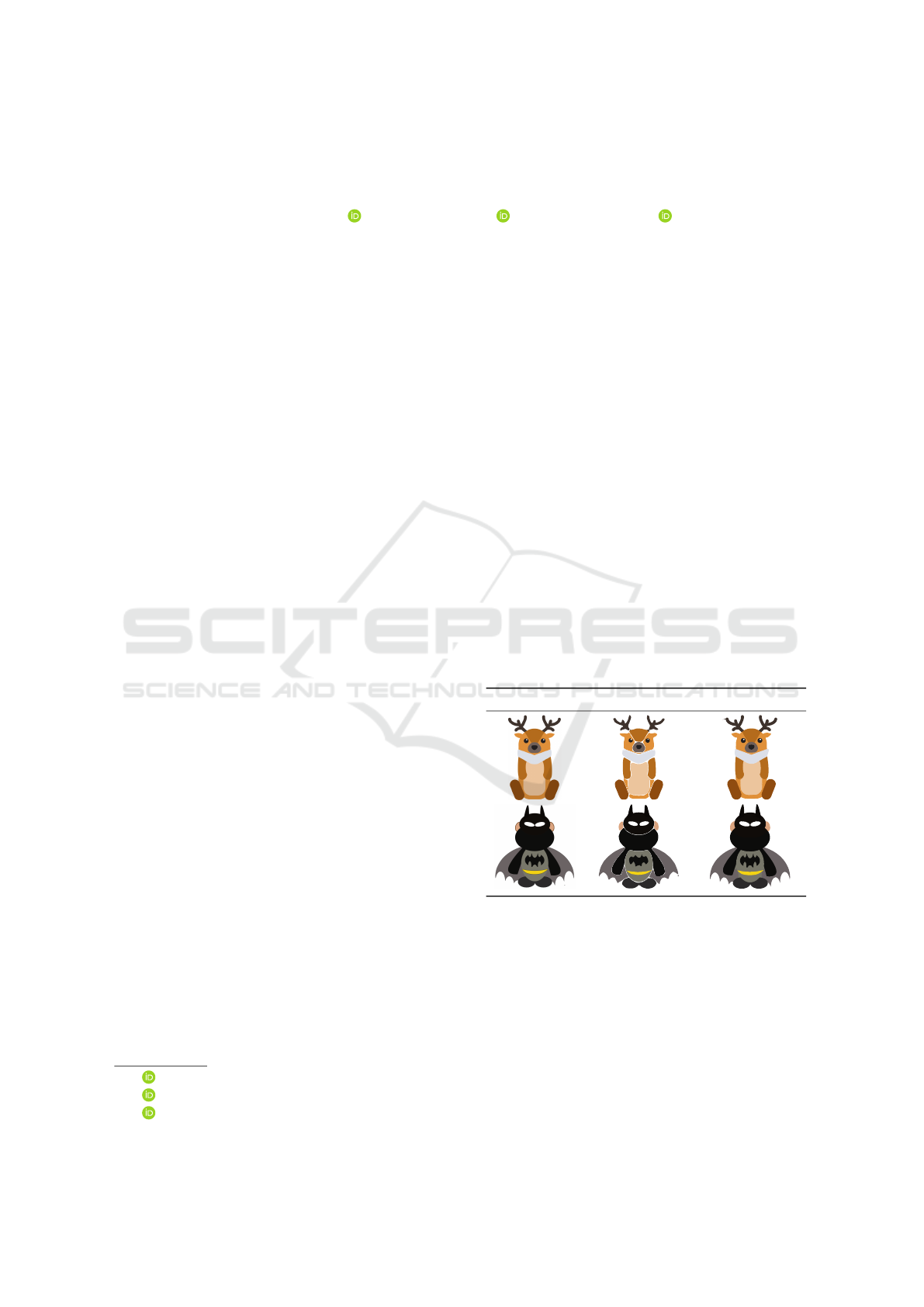
Target LIVE LIVBOC

Figure 3: Comparison of path efﬁciency between LIVE

and LIVBOC methods. LIVBOC assigns a single path per

shape, while LIVE generates multiple paths for the same

shape.

on the size of the shape contoured. This feature helps

LIVBOC to represent each shape with a single path,

even if this target shape is partially covered by other

shapes in the ground-truth image. By minimizing in-

formation duplication—where a single shape would

otherwise require multiple paths for representation (as

is the case with LIVE), LIVBOC reduces the size of

SVG output ﬁles, as shown in Figure 3 and evidenced

in Table 1. The generation of contour-based paths also

helps in reducing time needed for reaching the target

shape, therefore, reducing overall time of the vector-

ization process.

Visual Comparison. In Figure 4, we show the vector-

ization results for samples of different levels of com-

plexity.

In simple samples, while both methods give accu-

rate vectorization, LIVE still misses some important

paths, resulting in not only a lower perceptual quality

of the output image, but also in consuming a higher

number of paths and a larger storage for the output

ﬁle due to information duplication.

Medium samples show a clear superiority of the

LIVBOC performance where we can notice how

LIVE is generating overlapping shapes, where vec-

tors are newer covering previous correct ones, while

our method avoids that mistake thanks to the usage of

the overlap loss function.

Complex samples show the core point of power

of our method. One of the limitations of the LIVE

method observed during experiments is its tendency

to generate random paths when no further shapes are

available for vectorization. This behavior can de-

crease reconstruction ﬁdelity and lead to the loss of

perceptual quality. In contrast, the Bayesian opti-

mization step in LIVBOC enables it to consistently

identify missing paths, as demonstrated in complex

samples with ﬁne details.

As can be seen in Table 1, our LIVBOC method

signiﬁcantly reduces processing time compared to the

LIVE baseline, while at the same time, achieving sim-

ilar or better results in just 100 iterations versus the

500 iterations required by LIVE. This efﬁciency is

due to LIVBOC’s contour-based initialization, which

VISAPP 2025 - 20th International Conference on Computer Vision Theory and Applications

836

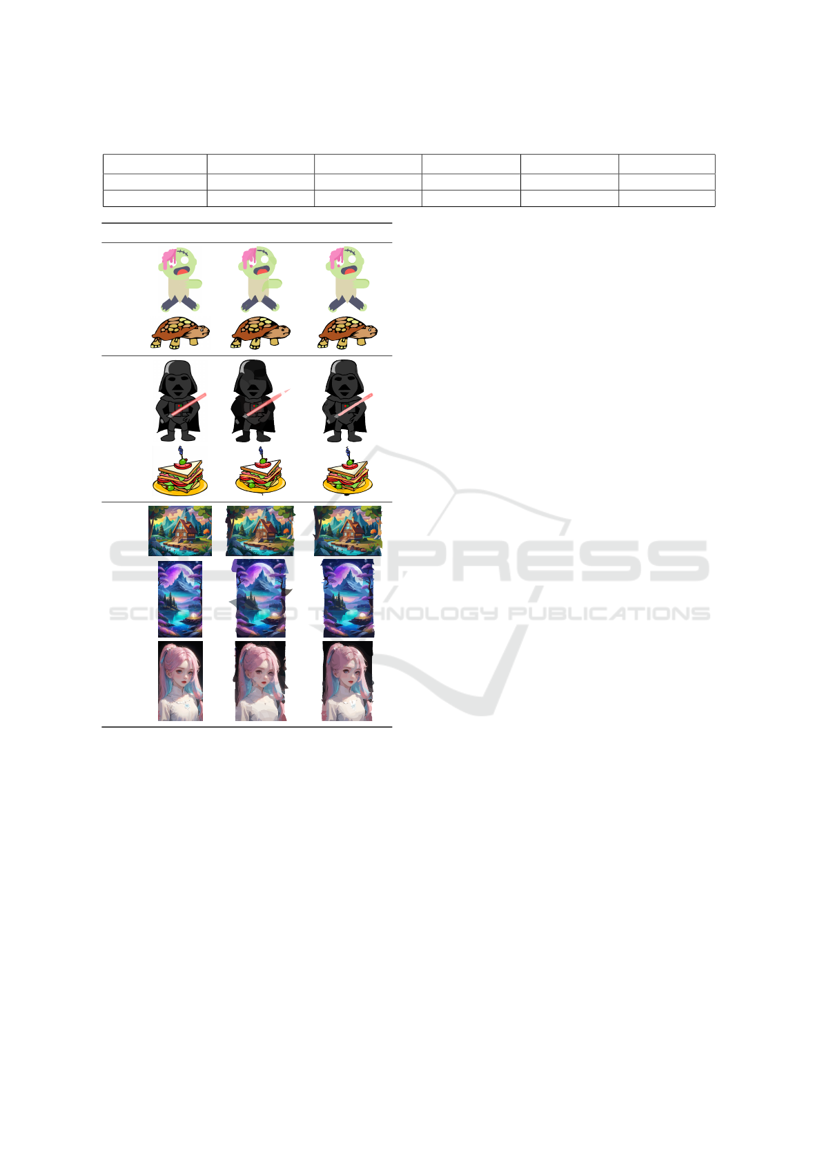
Table 1: Comparison between LIVE and our LIVBOC across 30 images of different paths’ complexity.

Metric L

(Mean ± SD) SSIM (Mean ± SD) Time, seconds File Size (KB) Path Number

LIVE 0.0107 ± 0.0069 0.8943 ± 0.0784 22470 62.5 99.34

LIVBOC (ours) 0.0056 ± 0.0038 0.9334 ± 0.0788 7802 56.48 46.05

Target LIVE LIVBOC (ours)

SimpleMediumComplex

Figure 4: Samples of LIVE and our method results on im-

ages of various complexities.

is optimized using Bayesian methods. In contrast,

LIVE initializes small Bezier paths using ﬁxed, non-

optimized parameter values, resulting in the need for

more reﬁnement for paths during optimization.

5 CONCLUSION

In this work, we have introduced LIVBOC, a novel

method for image vectorization that addresses key

challenges in path initialization, color assignment,

and optimization. With the Bayesian-contour-based

initialization strategy, LIVBOC achieves a signiﬁcant

reduction in computational overhead while maintain-

ing a better preservation of information and recon-

struction ﬁdelity. The method adaptively sets the

number of points required for each shape, providing

efﬁcient path generation that minimizes redundancy

and ﬁle size.

The experimental results indicate that LIVBOC

outperforms the baseline LIVE method in all key

metrics. LIVBOC achieves a lower L

loss, faster

processing times, and more compact SVG represen-

tations, all while requiring fewer paths to represent

complex images. Qualitative comparisons further

highlight LIVBOC’s ability to preserve intricate de-

tails and avoid artifacts, resulting in smoother and

more accurate vectorizations, thus, a user can manip-

ulate with vectors more easily.

These results establish LIVBOC as a robust and

efﬁcient alternative to existing methods, with applica-

tions in scalable vector graphics, digital design, and

computational graphics. Future work will focus on

enhancing the LIVBOC coloring capabilities. Specif-

ically, our goal is to implement and optimize more

advanced coloring techniques, such as gradients and

pattern-based ﬁlls, in addition to solid ﬁll.

ACKNOWLEDGMENTS

The research was supported by the ITMO University,

project 623097 ”Development of libraries containing

perspective machine learning methods”.

REFERENCES

Arbel

aez, P., Maire, M., Fowlkes, C., and Malik, J. (2011).

Contour detection and hierarchical image segmenta-

tion. IEEE Transactions on Pattern Analysis and Ma-

chine Intelligence, 33(5):898–916.

Bazhenov, E., Jarsky, I., Eﬁmova, V., and Muravyov, S.

(2024). Evovec: Evolutionary image vectorization

with adaptive curve number and color gradients. In

Affenzeller, M., Winkler, S. M., Kononova, A. V.,

Trautmann, H., Tu

sar, T., Machado, P., and B

ack,

T., editors, Parallel Problem Solving from Nature –

PPSN XVIII, pages 383–397, Cham. Springer Nature

Switzerland.

Dziuba, M., Jarsky, I., Eﬁmova, V., and Filchenkov, A.

(2023). Image vectorization: a review.

Layerwise Image Vectorization via Bayesain-Optimized Contour

837

Frackiewicz, M., Mandrella, A., and Palus, H. (2019). Fast

color quantization by k-means clustering combined

with image sampling. Symmetry, 11.

Frazier, P. I. (2018). A tutorial on bayesian optimization.

Hor

e, A. and Ziou, D. (2010). Image quality metrics: Psnr

vs. ssim. In 2010 20th International Conference on

Pattern Recognition, pages 2366–2369.

Hu, T., Yi, R., Qian, B., Zhang, J., Rosin, P. L., and Lai, Y.-

K. (2024). Supersvg: Superpixel-based scalable vec-

tor graphics synthesis.

Ma, X., Zhou, Y., Xu, X., Sun, B., Filev, V., Orlov, N.,

Fu, Y., and Shi, H. (2022). Towards layer-wise image

vectorization.

Nguyen, V. (2019). Bayesian optimization for accelerat-

ing hyper-parameter tuning. In 2019 IEEE Second In-

ternational Conference on Artiﬁcial Intelligence and

Knowledge Engineering (AIKE), pages 302–305.

Polewski, P., Shelton, J., Yao, W., and Heurich, M. (2024).

Segmenting objects with bayesian fusion of active

contour models and convnet priors.

Snoek, J., Larochelle, H., and Adams, R. P. (2012). Prac-

tical bayesian optimization of machine learning algo-

rithms.

Sorkine, O., Cohen-Or, D., Lipman, Y., Alexa, M., R

ossl,

C., and Seidel, H.-P. (2004). Laplacian surface

editing. In Proceedings of the 2004 Eurograph-

ics/ACM SIGGRAPH symposium on Geometry pro-

cessing, pages 175–184.

Vartziotis, D. and Himpel, B. (2014). Laplacian smoothing

revisited.

Wang, Z., Huang, J., Sun, Z., Cohen-Or, D., and Lu, M.

(2024). Layered image vectorization via semantic

simpliﬁcation.

Zhu, H., Chong, J. I., Hu, T., Yi, R., Lai, Y.-K., and Rosin,

P. L. (2023). Samvg: A multi-stage image vectoriza-

tion model with the segment-anything model.

VISAPP 2025 - 20th International Conference on Computer Vision Theory and Applications

838