Poly-MgNet: Polynomial Building Blocks in Multigrid-Inspired ResNets

Antonia van Betteray

, Matthias Rottmann

and Karsten Kahl

IZMD, University of Wuppertal, Germany

{vanbetteray, rottmann, kkahl}@uni-wuppertal.de

Keywords:

ResNets, Multigrid Methods, Polynomial Smoother, Accuracy-Weight Trade-Off.

Abstract:

The structural analogies of ResNets and Multigrid (MG) methods such as common building blocks like convo-

lutions and poolings where already pointed out by He et al. in 2016. Multigrid methods are used in the context

of scientiﬁc computing for solving large sparse linear systems arising from partial differential equations. MG

methods particularly rely on two main concepts: smoothing and residual restriction / coarsening. Exploiting

these analogies, He and Xu developed the MgNet framework, which integrates MG schemes into the design of

ResNets. In this work, we introduce a novel neural network building block inspired by polynomial smoothers

from MG theory. Our polynomial block from an MG perspective naturally extends the MgNet framework to

Poly-Mgnet and at the same time reduces the number of weights in MgNet. We present a comprehensive study

of our polynomial block, analyzing the choice of initial coefﬁcients, the polynomial degree, the placement of

activation functions, as well as of batch normalizations. Our results demonstrate that constructing (quadratic)

polynomial building blocks based on real and imaginary polynomial roots enhances Poly-MgNet’s capacity in

terms of accuracy. Furthermore, our approach achieves an improved trade-off of model accuracy and number

of weights compared to ResNet as well as compared to speciﬁc conﬁgurations of MgNet.

1 INTRODUCTION

Deep convolutional neural networks (CNNs) are

state-of-the-art methods for image classiﬁcation

tasks (Krizhevsky et al., 2012; Russakovsky et al.,

2015; He et al., 2015; Dosovitskiy et al., 2021). Es-

pecially ResNets (He et al., 2016a; He et al., 2016b;

Liu et al., 2022) have become increasingly popular,

as they successfully overcome the vanishing gradient

problem (Glorot and Bengio, 2010a).

Nevertheless these networks contain O(10

) –

O(10

) weights, thus being heavily over parameter-

ized. A reduction of the weight count is clearly de-

sirable, which, however, can result in an undesired

bias. This trade-off is referred to as “bias-complexity

trade-off” which constitutes a fundamental problem

of machine learning, see e.g. (Shalev-Shwartz and

Ben-David, 2014). In this work, we address this prob-

lem from a multigrid (MG) perspective. MG methods

are hierarchical solvers for large sparse systems of lin-

ear equations that arise from discretizations of par-

tial differential equations (Trottenberg et al., 2001).

The main idea of MG consists of two components,

https://orcid.org/0000-0002-2338-1753

https://orcid.org/0000-0003-3840-0184

https://orcid.org/0000-0002-3510-3320

namely a local relaxation scheme, which is cheap to

apply, but slow to converge as it lacks the possibility

to address global features. Thus it is complemented

with a coarse grid correction, that exploits a repre-

sentation of the problem formulation on a coarser

scale thus making long range information exchange

easier. In classical MG theory this complementarity

can be associated with the split of the error into geo-

metrically oscillatory and smooth functions. Where

the oscillatory part is quickly dampened by the lo-

cal relaxation scheme and the smooth part accurately

described and dealt with on coarser scales (Trotten-

berg et al., 2001). The authors of ResNet (He et al.,

2016a) already mentioned the inherent similarities be-

tween MG and residual layers. This structural con-

nection was further elaborated in (He and Xu, 2019),

where ResNets, composed of residual layers (repre-

senting the smoothers) and pooling operations (repre-

senting the coarse grid restrictions), are cast into a full

approximation scheme (FAS). The resulting frame-

work, termed MgNet, further exploits the similarity

to MG methods, in which the discretized operators

stemming from PDEs remain ﬁxed between consec-

utive coarsenings/poolings. This yields a justiﬁca-

tion for sharing weight tensors across multiple resid-

ual layers, e.g. ﬁg. 1(b) and ﬁg. 1(c), reducing the

van Betteray, A., Rottmann, M. and Kahl, K.

Poly-MgNet: Polynomial Building Blocks in Multigrid-Inspired ResNets.

DOI: 10.5220/0013382800003905

Paper published under CC license (CC BY-NC-ND 4.0)

In Proceedings of the 14th International Conference on Pattern Recognition Applications and Methods (ICPRAM 2025), pages 181-191

ISBN: 978-989-758-730-6; ISSN: 2184-4313

181

ℓ

i+1

ℓ

i+1

ℓ

(a) residual

ℓ

(k)

ℓ

−

ℓ

(k+1)

ℓ

−

(b) non-

stationary

ℓ

−

ℓ

−

ℓ

αℓ

(k+1)

−

ℓ

(k+1)

ℓ

−

(d) polynomial

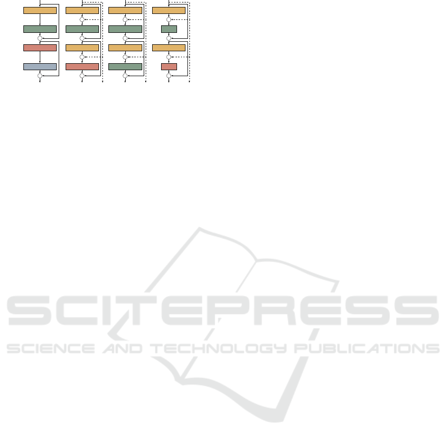
Figure 1: Weight sharing in ResNet and MgNet; (1a)

ResNet-blocks, no weight sharing; (1b) MgNet-blocks,

shared A

ℓ

; (1c) MgNet-blocks, shared layers A

ℓ

and B

ℓ

and

Poly-MgNet (ﬁg. 1d).

overall weight count of the network. A joint per-

spective of multigrid structures in all dimensions was

taken by (van Betteray et al., 2023), resulting in an

improved weight-accuracy trade-off and thus demon-

strates that ResNets are overparameterized.

In this work, we exploit additional structural sim-

ilarities between MG and residual networks to further

reduce the weight count of MgNet. A typical ResNet

block is built from two convolutions A and B gated

by a residual connection. Considering a given system

of linear equations Au = f , so-called MG smoothing

applies an operation B to the residual f −Au, i.e.,

u ← u + B( f −Au),

in order to improve u, i.e., reduce the residual, itera-

tively. In a nutshell, this operation has the property

of smoothing the error associated to the current ap-

proximation u. In MgNet, B is chosen as a learnable

convolution operator, but here we consider a cheaper

alternative that reuses the convolution A in its deﬁni-

tion. Again motivated by the linear-algebra analogy,

we consider polynomials p(A) for B with only a hand-

ful of learnable parameters, thus reducing the number

of parameters by almost 50%. A special case and the

simplest instance of this idea is the Richardson iter-

ation (Trottenberg et al., 2001) where B = ωI, with

I the identity matrix and ω a scalar. Clearly, we do

not want to limit ourselves to such trivial polynomials

and explore in this work to which extent smoothing

iterations using polynomial approximations are suit-

able within MgNet, e.g. ﬁg. 1(c), to further reduce the

number of weights.

We summarize our contribution as follows:

1. We introduce a new building block, to fur-

ther reduce the number of weights in multigrid-

inspired CNNs, such as MgNet. These meth-

ods are inspired by MG smoothers, namely block

smoothers, polynomial smoothers and Richard-

son smoothers, yielding layer modules of reduced

weight counts.

2. We implement this building block into MgNet

and show signiﬁcant reductions of weight counts

while almost maintaining classiﬁcation accuracy.

3. Our approach yields further insights into the

inherent connection of MG and ResNets and

demonstrates that MG methodology is useful for

the construction of weight-count-efﬁcient CNNs.

The remainder of this article is organized as fol-

lows: Section 2 discusses related works. In section 3

we elaborate on the similarities of residual networks

and MG, followed by the construction of our layers

inspired by MG smoothers. Ultimately numerical re-

sults are presented in section 4.

2 RELATED WORKS

In this section, we provide an overview of related

works, classiﬁed into four categories of approaches,

sorted from remotely to closely related.

Channel Reduction. The set of existing methods

for the reduction of weight counts and the set of exist-

ing methods to reduce the computational complexity

of CNNs have a signiﬁcant intersection. As one of

many possible approaches, a reduction of computa-

tional complexity can be achieved by a reduction of

the number of channels in convolutional layers. Con-

sidering the simpliﬁed case where the number of input

channels c equals the number of output channels of a

given convolutional layer and the ﬁlter extent s be-

ing equal in both directions, the number of weights of

such a layer is given by s

·c

. Thus, a reduction of c

results in a clear reduction of the number of weights.

In (Molchanov et al., 2016) it was shown experimen-

tally, that there is redundancy in CNNs, which al-

lows for cutting connections between channels after

the CNN has been trained. This process is known as

CNN pruning (Hassibi and Stork, 1992; Han et al.,

2015; Li et al., 2017). At the same time pruning and

other sparsity enhancing methods (Changpinyo et al.,

2017; Han et al., 2017) reduce the model complexity

in terms of weights. While these approaches ﬁrst train

a CNN to convergence, in (Gale et al., 2019) the CNN

is pruned periodically during training. In (Lee et al.,

2019) a saliency criterion to identify structurally im-

portant connections is proposed, which allows for

pruning before training. We also reduce the weight

count before training, however, our approach is based

on the inherent similarity of MG and ResNets, utiliz-

ing MG methodology to ﬁnd an explanation for more

weight count efﬁcient layer modules.

ICPRAM 2025 - 14th International Conference on Pattern Recognition Applications and Methods

182

A related research area is the ﬁeld of neural archi-

tecture search (Elsken et al., 2019; Cha et al., 2022),

where the goal is to search the space of architectures

close to optimal ones w.r.t. chosen optimization crite-

ria. If the focus is on computational efﬁciency, then

tuning the channel hyper-parameters is one of many

possible approaches (Gordon et al., 2017), resulting

in a reduction of weight count. While the aforemen-

tioned approaches use optimization procedures to re-

duce the number of weights, we utilize MG method-

ology that yields an explanation for the achieved efﬁ-

ciency.

Modiﬁed Layers. Another line of research ad-

dresses the speciﬁc construction of convolutional lay-

ers. Compared to the aforementioned approaches, the

constructions outlined in this section are based on hu-

man intuition and conventional methods to improve

computational efﬁciency. Also in this line of research,

there is a close connection between computational ef-

ﬁciency and the reduction of the number of weights.

One approach to reduce the number of weights is the

use of grouped convolutions (Krizhevsky et al., 2012;

Xie et al., 2017), where the channels are grouped

into g decoupled subsets, each convoluted with its

own set of ﬁlters, thus decreasing the weight count to





. This decoupled structure impedes the ex-

change of information across the channels. To over-

come this issue, e.g. in (Zhang et al., 2018) a com-

bination of groupings and channel shufﬂing, termed

ShufﬂeNet, has been proposed.

A combination of layers, which also allows for

a reduction in ﬂoating point operations, are so-

called depth-wise separable convolutions, introduced

in (Howard et al., 2017; Sandler et al., 2018; Howard

et al., 2019) as key feature for the MobileNet archi-

tecture: a depth-wise convolution, i.e., grouped con-

volution with g = c is followed by a point-wise 1 ×1

convolution, to create a linear combination of the out-

put of the former. This results in a reduced weight

count of s

+ 2c, i.e., each kernel slice of extent c

replaced by a rank - one approximation.

Polynomial Neural Networks. Polynomial neu-

ral networks are NNs that produce an output be-

ing a polynomial of the input. This approach was

ﬁrst pursued via the group method of data handling

(GMDH) (Oh et al., 2003). It determines the structure

of a polynomial model in a combinatorial fashion and

selects the best solution based on an external criterion,

e.g. least squares. While these methods belong to self-

organizing neural networks, another category consid-

ers the output of the network as a high-order poly-

nomial of the input (Shin and Ghosh, 1991; Chrysos

et al., 2020; Chrysos et al., 2022). Our goal is to uti-

lize polynomials as a building block in CNNs without

reframing their purpose to polynomial approximation.

Multigrid Inspired Architectures. In scientiﬁc

computing, MG methods are algorithms based on hi-

erarchical discretizations, to efﬁciently solve systems

of (non-)linear differential equations (PDEs) (Trot-

tenberg et al., 2001; Treister and Yavneh, 2011;

Kahl, 2009). Some works utilizes CNNs to solve

PDEs (Tomasi and Krause, 2021), e.g. by estimat-

ing optimal preconditioners (G

otz and Anzt, 2018) or

prolongation and restriction operators (Katrutsa et al.,

2017). Another line of research focuses on architec-

tures based on common computational components

as well as similarities of CNNs and MG (He et al.,

2016a). In (Ke et al., 2017) an architecture of pyramid

layers of differently scaled convolutional layers, with

each pyramid processing coarse and ﬁne grid repre-

sentations in parallel, is proposed. This MG archi-

tecture improves accuracy, while being weight-count

efﬁcient.

The close similarities between CNNs and MG

are further exploited in (He and Xu, 2019), where a

framework termed MgNet is introduced. It yields a

justiﬁcation for sharing weight tensors within convo-

lutions in subsequent ResNet blocks with the same

spatial extent. Utilizing MG in the spatial dimen-

sions, MgNet models have, compared to ResNets

with the same number of layers, fewer weights, while

maintaining classiﬁcation accuracy. An alternating

stack of MgNet blocks and poolings can be viewed

as the left leg of an MG V -cycle. Another hierar-

chical structure, however in the channel dimension,

is proposed in (Eliasof et al., 2020). Their building

block, termed multigrid-in-channels (MGIC), is built

on grouped convolutions and coarsening via channel

pooling. Utilizing MG in the channel dimensions,

this approach improves the scaling of the number of

weights with the number of channels from quadratic

to linear. A uniﬁed MG perspective is taken on both

the spatial and channel dimensions in (van Betteray

et al., 2023). The introduced architecture, called

multigrid in all dimensions (MGiaD), improves the

trade-off between the number of weights and accu-

racy via full approximation schemes in the spatial and

channel dimensions, including MgNet’s weight shar-

ing. Similarly to these approaches, we exploit the in-

herent similarities between CNNs and MG to further

reduce the weight count. Our focus in this work is to

cast MG smoothers into CNN layer modules, which

has not been studied in related work.

Poly-MgNet: Polynomial Building Blocks in Multigrid-Inspired ResNets

183

3 RESIDUAL NETWORKS AND

MULTIGRID METHODS

MG consists of two complementary components, the

smoother and the coarse grid correction. In a re-

cursive fashion, the coarse grid correction is typi-

cally treated by restricting/pooling in spatial dimen-

sions, then smoothing on the next coarser scale and

then applying another even coarser coarse grid cor-

rection, etc. This structure is already resembled by

typical CNNs which alternate between convolutions

and poolings. In MG and in CNNs, the smoother is

the main work step with the highest computational ef-

fort. A suitable choice of it is vital for the success of

an MG method and we will see that these ﬁndings are

beneﬁcial for CNNs as well. In this section we intro-

duce the smoother, the coarsening and unify the MG

and CNN perspective.

Revisiting ResNet and MgNet. Given a data-

feature relation A(u) = f , the right-hand-side f rep-

resents the data space and u the features. In CNNs, A

is learnable and A(u) = f can be optimized (He and

Xu, 2019). The mappings between data f ∈ R

m×n×c

and features u ∈ R

m×n×h

are given by

A : R

m×n×h

7→ R

m×n×c

, s.t. A(u) = f (1)

B : R

m×n×c

7→ R

m×n×h

, s.t. u ≈B( f ), (2)

where m and n characterize the spatial resolution di-

mensions of the input and c and h determine the di-

mension of the input and output channel respectively,

i.e. number of input and output channels can differ. A

can be considered as a feature-to-data map, while B is

applied to elements of the data space, is also referred

to as feature extractor. In MG the property u ≈ B( f )

is beneﬁcial for the method’s convergence, which will

be explained in the following. In the context of CNNs,

convolutional mappings usually are combined with

non-linear activation functions. For a clear presenta-

tion of the similarities between CNNs and MG, the

non-linearities are omitted for now. Considering a

large sparse system of linear equations A(u) = f , ob-

taining the direct solution u is not feasible. Therefore,

the true solution is iteratively approximated by

u. The

resulting error e = u −

u fulﬁlls the residual equation

r = f −A(

u) = A(u −

u) = Ae, (3)

where r is referred to as residual. Now, given an ap-

propriate feature extractor B, the approximated error

e = Br can be used to update the approximated solu-

tion

u ←

u +

e. Repeating this scheme with eq. (3)

yields a non-stationary iteration

u ← u + B

(k)

( f −A(u)) for k = 1,2,. .. (4)

to solve A(u) = f approximately. Hence, that fea-

ture extractors B

(k)

depend on iteration k, yet eq. (4)

can be turned into a stationary scheme with a ﬁxed

B, i.e. a shared weight tensor. On the other hand,

interpreting A as a data-feature mapping motivates a

ﬁxed A, i.e. also a shared weight tensor. As exam-

ined in (He and Xu, 2019) the structure of eq. (4),

with activation functions added, resembles a ResNet-

block. Combined with eq. (3) yields a non-stationary

iterative scheme. Explicitly, given the solution u

(k)

iteration k the residual

(k+1)

= f −Au

(k+1)

= (I −AB

(k)

(5)

is propagated to k + 1-th iteration and the coefﬁcient

(I −BA) equals a ResNet-block r

(k+1)

= r

(k)

+ BAr

(k)

(cf. ﬁg. 1a). The main difference between MgNet and

ResNet is sharing one or more weight tensors. Two

ResNet-blocks at one resolution level do not share

any weight tensors (cf. ﬁg. 1a). The weight count of

such two distinct blocks is given by 4 ·(s

×c ×h).

In MgNet, for the non-stationary case, i.e. only A is

shared, the weight count is reduced to 3 ·(s

×c ×h).

For the stationary case, i.e. sharing both A and B the

weight count for two blocks is only 2 ·(s

×c ×h).

The pseudo-inverse of A is generally a dense matrix,

which requires the representation as a fully connected

weight layer, but this conﬂicts with the required con-

volutional structure of the feature extractors B

(k)

(re-

spectively B). Even with an optimal choice of B

(k)

the convergence of the iteration eq. (4) is inevitably

slow, due to acting locally. However, convolutional

operators B

(k)

are computationally light. A few ap-

plications of the iteration have a smoothing effect on

features, and the resulting error can be accurately rep-

resented at a coarser resolution.

Resolution Coarsening. The restriction of the

(residual) data to coarser scales, facilitated by map-

pings

ℓ+1

ℓ

: R

ℓ

×n

ℓ

×c

ℓ

7→ R

ℓ+1

×n

ℓ+1

×c

ℓ+1

, (6)

yields a hierarchy of resolution levels ℓ = 1,.. . ,L. On

each level ℓ the smoothing iteration (4) can be applied

by resolution-wise mappings A

ℓ

and B

(k)

ℓ

, where on

each level ℓ initially u

(0)

ℓ

= 0. Note that the feature

extractors can also be stationary. Equivalent to re-

strictions in MG, in CNNs the resolution dimension

is reduced by pooling operations with stride greater

than 1. In CNNs usually the channel dimension is in-

creased in the process. Corresponding to the coarsen-

ing leg of a standard MG V -cycle (Trottenberg et al.,

2001), the combination of ν smoothing iterations on

each resolution level ℓ and L −1 restrictions yields al-

gorithm 1.

ICPRAM 2025 - 14th International Conference on Pattern Recognition Applications and Methods

184

ℓ

...







1 0 1 1

0 1 1 1

0 1 0 0

1 0 0 1







ℓ

ℓ+1

ℓ

ℓ+1

ℓ

Figure 2: Data-feature relations A

ℓ

and B

ℓ

on resolution

level ℓ followed by transfer to coarser resolution ℓ + 1.

ℓ

applied to the features u

ℓ

, calculation of the residual

ℓ

= f

ℓ

−A

ℓ

, on which the feature extractor B

ℓ

is applied.

Algorithm 1: \-MgNet( f

ℓ

Initialization: u

ℓ

= 0

1 for ℓ = 1,.. .,L do

2 for k = 1, ...,ν do

3 u

(k+1)

ℓ

= u

(k)

ℓ

+ B

(k)

ℓ

( f

ℓ

−A

ℓ

(k)

ℓ

))

4 end

5 u

(0)

ℓ+1

= 0

6 f

ℓ+1

= R

ℓ+1

ℓ

( f

ℓ

−A

ℓ

(ν)

ℓ

))

7 end

Full Approximation Scheme (FAS). So far acti-

vation functions, potential non-linear poolings and

normalization operations, which are characteristic of

CNNs, have been disregarded. However, if we now

take these into account, we obtain a non-linear over-

all structure for CNNs. The non-linearity in MG prob-

lems yields multiple possible minima, so that the ini-

tial solution not only determines the solution, but also

has a crucial inﬂuence on the convergence rate. Con-

sequently, an initial guess u

(0)

ℓ+1

at the coarser scale

determined by the current feature approximation u

ℓ

is likely to dominate u

(0)

ℓ+1

= 0. Therefore, the feature

approximations of non-linear problems are also pro-

jected to the coarser scale by a mapping

ℓ+1

ℓ

: R

ℓ

×m

ℓ

×c

ℓ

7→ R

ℓ+1

×m

ℓ+1

×c

ℓ+1

, (7)

to initialize the solution u

(0)

ℓ+1

= Π

ℓ+1

ℓ

(ν)

ℓ

. Given

this non-trivial initial solution on level ℓ + 1, the re-

stricted residual data f

ℓ+1

requires an adjustment by

ℓ+1

Accordingly, in algorithm 1 lines 5 and 6 are

changed to

(0)

ℓ+1

= Π

ℓ+1

ℓ

(ν)

ℓ

(8)

ℓ+1

= R

ℓ+1

ℓ

( f

ℓ

−A

ℓ

(ν)

ℓ

)) + A

ℓ+1

(0)

ℓ+1

). (9)

In the CNN context, the projection operation (7) cor-

responds to another pooling operation, but it has no

exact counterpart in the general ResNet architecture.

Figure 2 summarizes relevant mappings and schemes

the role of B

ℓ

as feature extractor, A

ℓ

as data-feature

mapping, followed by restriction and projection, re-

spectively.

3.1 Polynomial (Smoother) in Residual

Blocks

Thus far the iterative scheme, eq. (4), was either con-

sidered to be stationary or non-stationary with matri-

ces B

(k)

or B, respectively. Even though B is a rough

and computationally inexpensive approximation for

−1

, in order to achieve a reduction of the residual we

can further reduce the number of learnable weights

and increase the interpretability of B by replacing it

by a polynomial (smoother) p

(A) ≈ A

−1

of degree

d ∈ N

, i.e., the residual block then reads

u ← u + p

(A)( f −A(u)). (10)

In here p

is a polynomial

(A) =

∑

i=0

. (11)

with (learnable) coefﬁcients α

. In the case of polyno-

mial smoothers (B = p

(A)), the non-stationary case

is considered, e.g. only weight tensor A is shared. Fur-

thermore these models are denoted by MgNet

In order to ease the following discussion note that

under the assumption that A is diagonalizable, i.e.,

A = XΛX

−1

with a matrix X containing the eigen-

vectors of A as its columns and a diagonal matrix Λ

of eigenvalues, we ﬁnd

(A) =

∑

i=0

= X

∑

i=0

−1

. (12)

Thus the action of the polynomial on a matrix A is de-

termined solely by the evaluation of the scalar poly-

nomial p

with coefﬁcients α

on the eigenvalues of

A. As it alleviates notation we are thus considering

the polynomial p

both as a scalar polynomial and

a matrix valued polynomial using the same notation.

Moreover, from now on for clarity in notation, let Λ

denote the spectrum of A.

Residual Blocks as Polynomials. Let B = p

(A) be

a polynomial feature extractor, than the residual equa-

tion 3 yields

(k+1)

= (I −Ap

(A))r

(k)

= q

d+1

(A)r

(0)

, (13)

where the factor (I −Ap

(A)) itself is a polynomial

d+1

(A) of degree d + 1. Hence, using eq. (11) we

ﬁnd

d+1

(A) = I −Ap

(A) = I −

∑

i=0

i+1

. (14)

and see that q

d+1

is normalized with a constant co-

efﬁcient equal to 1, i.e., q

d+1

(0) = 1, which implies

Poly-MgNet: Polynomial Building Blocks in Multigrid-Inspired ResNets

185

that residual components belonging to kernel modes

of A are unaffected by such a polynomial correction

approach

. Leveraging the normalization of q

d+1

obtain its decomposition into a product of linear fac-

tors as

d+1

(A) =

d+1

∏

i=1

(I −

A) with q

d+1

(ζ

) = 0 and ζ

∈C.

(15)

That is, instead of learning the coefﬁcients α

we can

equivalently learn the roots of the polynomial q

d+1

While it is not immediately clear how α

need to be

chosen to ensure p

(A) ≈A

−1

to obtain a reduction of

the residual, the roots of the polynomial q

d+1

have an

immediate interpretation with respect to the reduction

of the residual. Again assuming that A is diagonal-

izable and taking into account that polynomials tend

to be small only close to their roots. That is, writing

(k)

∑

as a linear combination of the eigenvec-

tors of A we ﬁnd

d+1

(A)r

(k)

∑

d+1

∏

i=1



1 −



, (16)

which is small, if the roots ζ

capture the distribution

of the eigenvalues of A correctly. To be more spe-

ciﬁc it is clear that roots close to the boundaries of the

spectrum of A, Λ ⊆C, are required in order to prevent

catastrophic over correction of the respective eigen-

components of the residual (Saad, 2003)(cf. ﬁg. 4).

Yet, the aim of minimizing the residual is consis-

tent with keeping the polynomial within the spectrum

small. To that end eigenvalues located at the spec-

trum’s boundary are chosen as roots for the polyno-

mial. Obviously A

̸= A holds, which yields guaran-

teed complex conjugated pairs of eigenvalues. This

can be used to construct a polynomial in linear factor

representation, covering the extend of the real axis,

e.g. ﬁg. 4, and quadratic terms, covering the extend of

the imaginary area and avoiding complex arithmetic

within the CNN at the same time

The residual propagation eq. (3) for a pair of com-

plex conjugated eigenvalues z and ¯z yields

(k+1)

= (1 −

A)(1 −

¯z

A)r

(k)

= ˜q

d+1

(k)

(17)

where ˜q

d+1

itself is a quadratic polynomial of degree

d + 1 with roots z = a+ib and its complex conjugated

counterpart ¯z with i the imaginary unit. Thus, the re-

sulting polynomial is the product of m linear polyno-

mials ˆq

and n quadratic polynomials ˜q

Clearly such modes are not affected in a general resid-

ual block with a (full) parameter matrix B either.

E.g. nn.ReLU does not support complex values, c.f.

issues #47052, #46642.

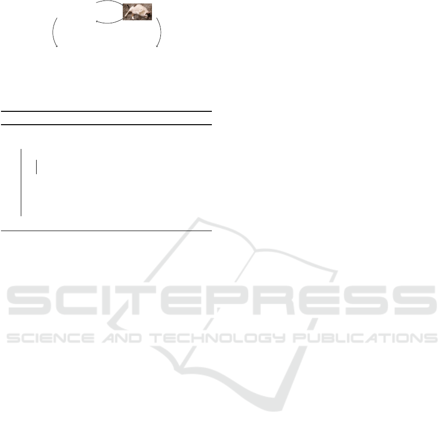
Figure 3: Surface representation of the spectrum Λ for the

corresponding matrix A ∈ R

64×64×3×3

. The x-axis repre-

sents the real parts, while y-axis corresponds to the imagi-

nary part. The z-axis illustrates the amplitude of the polyno-

mial function of abs(q

(Λ)), which has roots at the eigen-

values with minimal and maximal real parts, as well as the

and complex conjugated pair of eigenvalues with the max-

imal imaginary part. This visualization allows for an intu-

itive identiﬁcation of the spectrum’s maximal amplitude.

m+2n

(A) =

∏

i=1

ˆq

(A) ·

∏

j=1

˜q

(A), (18)

s.t. m + 2n.

The second observation revolves around the fact

that the decomposition of q

d+1

into a product of linear

factors can be viewed as a sequence of linear resid-

ual blocks, i.e., one residual block with B = ˆp

(A) is

equivalent to d + 1 residual blocks with B

(k)

/ζ

The quadratic terms also can be viewed as a sequence

of pairs of linear residual blocks, i.e. two residual

blocks with B = ˆq

are equivalent to B

(k)

/z and

(k+1)

/¯z respectively. The focus of our work is

on the polynomial perspective of a residual block, de-

noted by q. The iteration can be rewritten as

(k+1)

= u

(k)

+ (

+ b

−

+ b

)Ar

(k)

. (19)

For the ease of notation from now on the degree

of a polynomial q

is d. Consequently the degree

of a polynomial p is d − 1. Furthermore combin-

ing eq. (10) with eq. (18) results in a polynomial ver-

sion of MgNet, referred to as Poly-MgNet, which is

outlined in algorithm 2.

Due to observations made in our experiments

we limit the polynomial with linear factors, i.e. ˆq

in eq. (18) to m = 2. To cover the extent of the spec-

trum on the real axis we choose the real part (ℜ) of

eigenvalues with smallest and biggest real part for

the polynomial roots, i.e. ζ

(1)

= minℜ(Λ) and ζ

(2)

ICPRAM 2025 - 14th International Conference on Pattern Recognition Applications and Methods

186

Algorithm 2: Poly-\-MgNet( f

ℓ

Initialization: u

(0)

= 0

1 for ℓ = 1,.. .,L do

2 for k = 1, ...,m do

3 u

(k+1)

ℓ

= u

(k)

ℓ

(k)

ℓ

( f

ℓ

−A

ℓ

(k)

ℓ

))

4 end

5 u

ℓ

= u

(m)

6 for k = m + 1, ..., n do

7 z = ζ

(k)

ℓ

∈ C

8 a = ℜ(ζ

(k)

),b = ℑ(ζ

(k)

)

9 r

(k)

= f

ℓ

−Au

(k)

ℓ

10 u

(k+1)

ℓ

= u

(k)

ℓ

(2a −A)r

(k)

11 end

12 u

ℓ+1

= Π

ℓ+1

ℓ

(m+n)

ℓ

13 f

ℓ+1

= R

ℓ+1

ℓ

( f

ℓ

−A

ℓ

)) + A

ℓ+1

)

14 end

maxℜ(Λ) as polynomial coefﬁcients α

(k)

/ζ

(k)

Models with polynomial building blocks with a poly-

nomial degree d = m = 2 are denoted by MgNet

For degrees d ≥ 4 the roots for the quadratic polyno-

mials ˜q

are chosen as follows. For a single quadratic

term ˜q

, z = argmax(ℑ(Λ)) is the eigenvalue with

biggest imaginary part (ℑ), and ¯z its complex coun-

terpart. For polynomials of higher degrees we con-

tinue to choose roots, that are located at the border

of the spectrum to satisfy the requirement of small

polynomial values. The roots calculated for a poly-

nomial with degree d = 4 are deployed in the result-

ing polynomial q

(A) followed by its evaluation on

Λ. Consequently, the spectrum is a plane spanned

over the roots, e.g. shown in ﬁg. 3. The biggest eigen-

value w.r.t. the imaginary part, and its complex coun-

terpart are chosen as roots for q

(A). This recursion

of spanning the spectrum on the roots to determine

new maxima can be repeated as often as required, as

summarized in algorithm 3. The resulting models are

denoted by Poly-MgNet

Another observation is that enhancing the im-

pact of the real valued coefﬁcients by constructing a

quadratic version of ˆq in eq. (18), s.t.

(k+1)

= (I −αA

(k)

= ˆg

(k)

(20)

has a beneﬁcial impact on accuracy. Omitting it-

eration indices, a polynomial ˆg(A

) with coefﬁ-

cient α has roots at ±

√

. Corresponding to the

idea to keep the polynomial small within the spec-

trum we chose the coefﬁcient α =

with ζ

max(|max(ℜ(Λ))|,|min(ℜ(Λ))|) to ensure that the

root is at least at the border (or beyond) of the spec-

Algorithm 3: Roots ζ

for polynomials d ≥ 6.

Initialization:

(1)

= max(ℜ(Λ))

(2)

= min(ℜ(Λ))

(3)

= argmax(ℑ(Λ)), ζ

= ζ

(3)

1 for d = 6,8, . .. do

2 q

∏

d−2

k=1

(1 −

(k)

Λ)

3 ζ

(d−1)

= argmax(|q

(Λ)|)

4 ζ

(d)

= ζ

(d−1)

5 end

trum. Note that the degree of the overall polynomial

is now d = 2m + 2n. Consequently eq. (18) is

rewritten as

2m+2n

(A) =

∏

i=1

ˆg

) ·

∏

j=1

˜q

(A), (21)

and models that include the reinforced real part poly-

nomial g are denote by Poly-MgNet

. The following

discussions refer to ˆq

, although they can be applied

without restriction fo ˆg

To ReLU or not to ReLU Thus far we ignored the

fact, that typically regular ResNet-blocks are build

with rectiﬁed linear unit (ReLU) activation functions

σ = max(0,x). In ResNet, as depicted in ﬁg. 1, ev-

ery convolution A, B is followed by ReLU, which

also applies for MgNet, independent of shared opera-

tions. Furthermore this setting is applied in the special

case B = p

d−1

(A), especially for d = 1. The iterative

scheme with ReLU functions σ are given by

(k+1)

= u

(k)

+ σ p

d−1

(A)σ( f −Au

(k)

) (22)

However, our polynomial view on residual blocks

collides with the fact that the max-function typically

cannot be a term of a polynomial. Nevertheless ReLU

has a major inﬂuence on a high expressiveness of

CNNs which prompts us to review ReLU placements

in our polynomial residual blocks. To peruse the ac-

tual idea of ReLU-free polynomials a single ReLU is

applied on every resolution, namely before resolution

coarsening level, s.t. the initial solution is given by

(0)

ℓ+1

= Π

ℓ+1

ℓ

σu

(ν)

ℓ

(23)

where ν = m + n blocks denotes a polynomial degree

d = m + 2n. In our experiments we found, that given

this setting our models are not able to explain enough

non-linearity from the data resulting in a loss in accu-

racy. To regain expressive capacity of our polynomial

models towards data non-linearity, we placed ReLU

after calculating the residual

(k+1)

= u

(k)

+ p

d−1

(A)σ( f −Au

(k)

), (24)

Poly-MgNet: Polynomial Building Blocks in Multigrid-Inspired ResNets

187

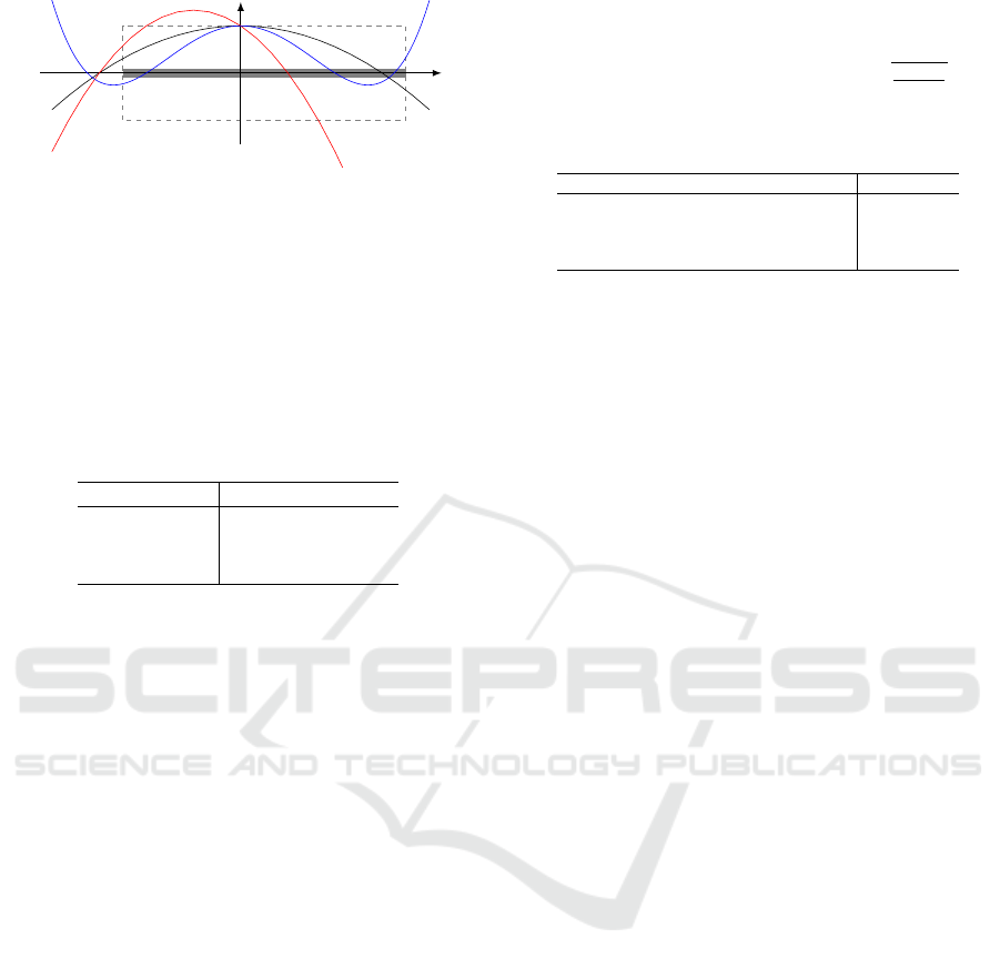
Figure 4: Schematic illustration of polynomials q

, (two

blocks), with different choices of roots from an exemplary

(real) spectrum.

which showed to be beneﬁcial to the models perfor-

mances. Furthermore the combination of eq. (23)

and eq. (24) showed to be the most beneﬁcial for

the accuracy. The introduced options are summarized

in table 1. Another question of interest is the place-

Table 1: Overview over possible placements of ReLU func-

tions σ in a polynomial block u ←u + p

d−1

(A)r.

σu

(ν)

ℓ

σp

d−1

(A) σr

eq. (22) × ×

eq. (23) ×

eq. (24) ×

eq. (23) + eq. (24) × ×

ment of batch normalization operations (bn) within

the polynomials. While their role is not completely

clear, we found, that different placements have inﬂu-

ence on the classiﬁcation accuracy of the correspond-

ing model. Although bn is typically applied before

ReLU, it is not required. In the following section, we

analyze and discuss various MgNet

bn and ReLU

conﬁgurations to identify the most effective setup.

4 EXPERIMENTAL RESULTS

We study the effect of our polynomial building blocks

(A) on the accuracy-weight trade-off by evaluating

the corresponding models on CIFAR-10. We report

the weight count and mean train and test accuracy

with standard deviation (std.) of three runs. Although

Poly-MgNet is robust to different coefﬁcient initial-

izations, cf. table 2, we initialize the coefﬁcients of

our models based on the spectrum of the convolutions

to align with our underlying intuition.

Experimental Setup. Our models are implemented

in Pytorch (Paszke et al., 2019). We train our mod-

els in batches of 128 for 400 epochs and use an op-

timizer based on stochastic gradient descent with a

momentum of 0.9 and a weight decay of 10

−4

. The

initial learning rate is set to 0.05 which is adapted by

a cosine-annealing scheduler (Loshchilov and Hutter,

2017).

Table 2: Inﬂuence of coefﬁcient initialization for mod-

els Poly-MgNet

and Poly-MgNet

. The coefﬁcients

are drawn either uniformly from the spectrum Λ. s.t.

U(λ

min

,λ

max

) or from U(−t,t) with t =

out

. The

latter follows the Xavier uniform distribution, which

is the standard approach for initializing convolutional

weights (Glorot and Bengio, 2010b).

Dataset polynomial initialization acc (± std)

CIFAR-10 q

U(λ

min

,λ

max

) 94.89 (0.16)

Xavier 94.76 (0.16)

U(λ

min

,λ

max

) 95.28 (0.19)

Xavier 95.32 (0.13)

Weight Count of Residual Blocks. As the weight

tensor A is shared across the polynomial blocks in our

approach the only learnable parameter is the single

polynomial coefﬁcient α

(k)

ℓ

/ζ

(k)

ℓ

, which is associ-

ated to each block. A polynomial of degree d only

incurs d parameters and it is thus essentially for free

to increase the polynomial degree w.r.t. the number of

parameters.

More speciﬁcally, let ν be the number of polyno-

mial building blocks on one resolution level ℓ and let

the size of the weight tensor be given by s

×c

, then

the weight count of different types of residual blocks

and polynomial setting is given as follows :

• ResNet18: (s

×c

) ·2 ·ν,

• MgNet

: (s

×c

) ·(1 + ν),

• MgNet

: (s

×c

) ·2,

• MgNet

: (s

×c

) + ν.

A regular ResNet18 block is built from 2 residual

blocks on 4 resolution levels with [64,128, 256, 512]

channels. The overall weight count of ResNet18 is

11.2 million (M). The corresponding MgNet

A,B

has

the same number of resolution levels, but according

to (He and Xu, 2019), the number of channels on the

fourth layer is reduced to 256. This setting results

in an overall weight count of 2.7M weights. Poly-

MgNet

with the same number of resolution levels

has a weight count of 1.3M.

ReLU Placement. In this section we examine the

different options for the placement of activation func-

tions and batch normalizations for polynomials q

corresponding to eq. (18) and g

, g

and g

, corre-

sponding to eq. (21) on CIFAR-10 to determine suit-

able settings. In table 1 the ReLU combinations we

determined as the most relevant are summarized. The

impact of these combinations on the accuracy of Poly-

MgNet

are compared in table 3. Recall that q

corresponds to ˆq

in eq. (18) and is linear with real-

valued roots. We observe that placing ReLU and bn at

the same places as in MgNet

A,B

, i.e. both A and B are

followed by ReLU and bn, leads to a lower accuracy

ICPRAM 2025 - 14th International Conference on Pattern Recognition Applications and Methods

188

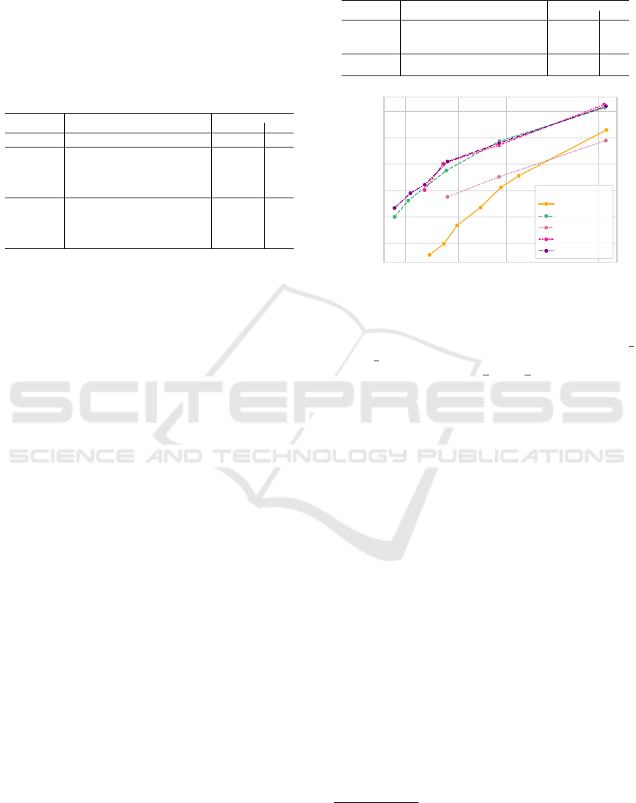
Table 3: Inﬂuence of ReLU and bn placement (cf.table 1) on

the accuracy of Poly-MgNet

and Poly-MgNet

trained on

CIFAR-10. The best accuracy for each model is highlighted

in bold. In the blocks corresponding to eq. (22) each ReLU

is followed by bn (ﬁrst row). For Poly-MgNet

we con-

sider the naive placement of one ReLU before resolution

coarsening, i.e. after the polynomial q

cf. eq. (23), we con-

trast this to an additional bn after ReLU with bn after the

residual r (row 2, 3). For Poly-MgNet

we limit the shown

results to the one with highest accuracy.

Model bn

σu

(ν)

ℓ

bn σp

d−1

(A) bn σr

accuracy

test (±std) train

MgNet

A,B

95.94 (0.27) 97.60

Poly-MgNet

× × 65.27 (63.4) 64.61

× × × × 93.04 (0.19) 94.00

× × × × 94.38 (0.35) 96.54

× × × 94.89 (0.16) 97.03

× × × 94.71 (0.21) 94.71

Poly-MgNet

× × 94.65 (0.33) 96.70

× × × × 95.28 (0.19) 97.23

× × × × 95.02 (0.18) 97.13

× × × × 95.04 (0.09) 97.11

× × × 95.00 (0.18) 97.11

than MgNet

A,B

. Furthermore the naive approach with

a single ReLU and no additional bn (eq. (23)) (on one

resolution level) is not robust, cf. table 3. One out of

three experimental runs fails to learn, resulting in a

low average accuracy with high standard deviation. It

is well known that polynomials suffer from instabil-

ities with increasing degree. In our experiments, we

observed in general that higher polynomial degrees

(greater than eight) often led to instabilities. Poly-

nomials of moderate degree mostly achieved superior

accuracy.

In contrast to that, the same ReLU placement

paired with bn applied after the calculation of the

residual achieves the highest mean accuracy, cf. ta-

ble 3. Furthermore, we study the ReLU placement

in Poly-MgNet

, which is based on polynomials,

that are quadratic in the real valued term. Note that

= ˆg

according to eq. (21). This emphasize on the

real-valued part increases the accuracy by 0.4 percent-

age points (pp), cf. table 3.

Selected results for the ReLU placement in mod-

els with polynomials g

and g

are summarized in ta-

ble 4. Recall, that polynomials with d > 2, and

respectively d > 4 are composed of a real valued

part and an imaginary valued part w.r.t. their roots;

cf. eq. (18). Speciﬁcally, the composition of g

given by g

= ˆg

) · ˆg

) · ˜q

(A). For the ˆg-terms

the placement of ReLU and bn follows the optimal

conﬁguration of g

determined in table 3.

We observe that for both Poly-MgNet

and Poly-

MgNet

that the application of ReLU and bn after the

residual update are essential for high accuracy.

Channel Scaling. After determining feasible set-

tings for the placements of ReLU and bn, we study

the inﬂuence of the capacity in terms of weights on

Table 4: Inﬂuence of ReLU and bn placement in Poly-

MgNet

and Poly-MgNet

on the accuracy.

Model bn

σu

(ν)

ℓ

bn σp

d−1

(A) bn σr

accuracy

test (±std) train

Poly-MgNet

× × × × 95.25 (0.41) 97.29

× × × × 95.55 (0.07) 97.34

× × × × 95.23 (0.13) 97.17

Poly-MgNet

× × × × 95.33 (0.33) 97.35

× × × × 95.60 (0.34) 97.4

0.8 1.6 3 10

Number of weights [M]

94.0

94.5

95.0

95.5

96.0

96.5

Accuracy (%)

Base Model

ResNet

MgNet

Poly-MgNet

Figure 5: Accuracy-weight trade-off of ResNet and MgNet

models: inﬂuence of overall capacity of residual networks

on classiﬁcation accuracy. The number of channels in the

residual blocks of ResNet and MgNet

A,B

are scaled by

√

and

√

8. In contrast, the channels of Poly-MgNet

are

rescaled by multiplying by

√

2 and

√

the accuracy of our Poly-MgNet models. To this end,

we introduce a channel scaling parameter to increase

the number of weights in Poly-MgNet according to

the weight count of ResNet and MgNet. Respectively,

we scale the channels of ResNet and MgNet to meet

the capacity of Poly-MgNet. Speciﬁcally, the overall

initial number of channels

is multiplied by a channel

scaling parameter λ < 1, to reduce the overall weight

count to a target limit of 1.3M weights, which cor-

responds to the average weight count of polynomial

MgNet models. The results are depicted in ﬁg. 5. A

regular ResNet18 has over 11M weights and achieves

an accuracy over 96%. Limiting the total weight

count to 1.3M – representing a reduction of more than

a factor 8 – results in an accuracy drop about 2 pp. In

contrast, the standard MgNet

A,B

with 2.7M weights

already achieves a reduction by a factor of 4 com-

pared to ResNet18 while maintaining competitive ac-

curacy. Despite the lower weight count, MgNet

A,B

still achieves an accuracy of 96%. When the weight

count of MgNet is reduced to 1.3M, we observe a loss

in accuracy of 0.6 pp. These ﬁndings highlight that,

compared to ResNet, the weight count can be drasti-

cally reduced without signiﬁcantly affecting the per-

Initial number of channels in the residual blocks for

ResNet18 is [64,128,256,512] and [64, 128, 256,256] for

MgNet

Poly-MgNet: Polynomial Building Blocks in Multigrid-Inspired ResNets

189

formance in terms of accuracy.

Our initial Poly-MgNet utilizes around 1.3M

weights. With this capacity Poly-MgNet

achieves

an accuracy of 94.89%. Compared to ResNet18,

which has over 11M weights, this represents a re-

duction in weight count by a factor of more than

8.5, while sacriﬁcing less than 1.5 pp of accuracy.

Poly-MgNet

and Poly-MgNet

achieve accuracies

over 95.5% with an initial capacity of approximately

1.4M weights, slightly improving the accuracy of

MgNet

A,B

by 0.13 pp while requiring identical capac-

ity. By increasing the number of channels for both

MgNet

A,B

and Poly-MgNet with building blocks g

and g

, all models achieve an accuracy of approx-

imately 96.60%, thereby drastically improving the

accuracy-weight trade-off compared to the standard

ResNet18.

5 CONCLUSION

In this work, we introduced Poly-MgNet, which com-

plements MgNet by a new network building block

inspired by polynomial MG smoothers. We con-

ducted comprehensive numerical studies on our build-

ing block, including baseline comparisons and several

ablations. More speciﬁcally, in comparison to MgNet

we found more favorable trade-offs between the num-

ber of weights in Poly-MgNet and the achieved ac-

curacy. In our ablation studies, we found that the

incorporation of multiple batch normalizations and

ReLU activation functions within a single building

block is crucial for achieving high accuracy, despite

the counterintuitive use of non-linearities in polyno-

mials. Additionally, we observed that building blocks

utilizing quadratic polynomials provide notable ben-

eﬁts in terms of accuracy. We make our code for re-

production of all experiments publicly available under

https://github.com/vanbetteray/Poly-MgNet.

ACKNOWLEDGEMENTS

This work is partially supported by the German Fed-

eral Ministry for Economic Affairs and Climate Ac-

tion, within the project “KI Delta Learning” (grant

no. 19A19013Q). M.R. acknowledges support by the

German Federal Ministry of Education and Research

within the junior research group project “UnrEAL”

(grant no. 01IS22069). The contribution of K.K. is

partially funded by the European Union’s HORIZON

MSCA Doctoral Networks programme project AQTI-

VATE (grant no. 101072344).

REFERENCES

Cha, S., Kim, T., Lee, H., and Yun, S.-Y. (2022). Super-

net in neural architecture search: A taxonomic survey.

ArXiv, abs/2204.03916.

Changpinyo, S., Sandler, M., and Zhmoginov, A. (2017).

The Power of Sparsity in Convolutional Neural Net-

works. ArXiv.

Chrysos, G. G., Moschoglou, S., Bouritsas, G., Deng, J.,

Panagakis, Y., and Zafeiriou, S. (2022). Deep polyno-

mial neural networks. IEEE Transactions on Pattern

Analysis and Machine Intelligence, 44(8):4021–4034.

Chrysos, G. G., Moschoglou, S., Bouritsas, G., Panagakis,

Y., Deng, J., and Zafeiriou, S. (2020). P-nets: Deep

polynomial neural networks. In Proceedings of the

IEEE/CVF Conference on Computer Vision and Pat-

tern Recognition (CVPR).

Dosovitskiy, A., Beyer, L., Kolesnikov, A., Weissenborn,

D., Zhai, X., Unterthiner, T., Dehghani, M., Minderer,

M., Heigold, G., Gelly, S., Uszkoreit, J., and Houlsby,

N. (2021). An image is worth 16x16 words: Trans-

formers for image recognition at scale. In Interna-

tional Conference on Learning Representations.

Eliasof, M., Ephrath, J., Ruthotto, L., and Treister, E.

(2020). Mgic: Multigrid-in-channels neural network

architectures. SIAM J. Sci. Comput., 45:S307–S328.

Elsken, T., Metzen, J. H., and Hutter, F. (2019). Neural

architecture search: A survey. J. Mach. Learn. Res.,

20(1):1997–2017.

Gale, T., Elsen, E., and Hooker, S. (2019). The state of spar-

sity in deep neural networks. CoRR, abs/1902.09574.

Glorot, X. and Bengio, Y. (2010a). Understanding the dif-

ﬁculty of training deep feedforward neural networks.

In International Conference on Artiﬁcial Intelligence

and Statistics.

Glorot, X. and Bengio, Y. (2010b). Understanding the difﬁ-

culty of training deep feedforward neural networks. In

Teh, Y. W. and Titterington, M., editors, Proceedings

of the Thirteenth International Conference on Artiﬁ-

cial Intelligence and Statistics, volume 9 of Proceed-

ings of Machine Learning Research, pages 249–256,

Chia Laguna Resort, Sardinia, Italy. PMLR.

Gordon, A., Eban, E., Nachum, O., Chen, B., Yang, T.-

J., and Choi, E. (2017). Morphnet: Fast & simple

resource-constrained structure learning of deep net-

works. 2018 IEEE/CVF Conference on Computer Vi-

sion and Pattern Recognition, pages 1586–1595.

otz, M. and Anzt, H. (2018). Machine learning-aided

numerical linear algebra: Convolutional neural net-

works for the efﬁcient preconditioner generation. In

2018 IEEE/ACM 9th Workshop on Latest Advances in

Scalable Algorithms for Large-Scale Systems (scalA),

pages 49–56.

Han, S., Pool, J., Narang, S., Mao, H., Gong, E., Tang, S.,

Elsen, E., Vajda, P., Paluri, M., Tran, J., Catanzaro,

B., and Dally, W. (2017). DSD: Dense-Sparse-Dense

Training for Deep Neural Networks. ICLR.

Han, S., Pool, J., Tran, J., and Dally, W. (2015). Learn-

ing both Weights and Connections for Efﬁcient Neural

Network. NIPS.

ICPRAM 2025 - 14th International Conference on Pattern Recognition Applications and Methods

190

Hassibi, B. and Stork, D. (1992). Second order derivatives

for network pruning: Optimal brain surgeon. In Han-

son, S., Cowan, J., and Giles, C., editors, Advances

in Neural Information Processing Systems, volume 5.

Morgan-Kaufmann.

He, J. and Xu, J. (2019). MgNet: A uniﬁed framework of

multigrid and convolutional neural network. Science

China Mathematics, 62(7):1331–1354.

He, K., Zhang, X., Ren, S., and Sun, J. (2015). Delving

Deep into Rectiﬁers: Surpassing Human-Level Per-

formance on ImageNet Classiﬁcation. In 2015 IEEE

International Conference on Computer Vision (ICCV),

pages 1026–1034, Santiago, Chile. IEEE.

He, K., Zhang, X., Ren, S., and Sun, J. (2016a). Deep

Residual Learning for Image Recognition. In 2016

IEEE Conference on Computer Vision and Pattern

Recognition (CVPR), pages 770–778. ISSN: 1063-

6919.

He, K., Zhang, X., Ren, S., and Sun, J. (2016b). Identity

mappings in deep residual networks. In Leibe, B.,

Matas, J., Sebe, N., and Welling, M., editors, Com-

puter Vision – ECCV 2016, pages 630–645, Cham.

Springer International Publishing.

Howard, A., Sandler, M., Chen, B., Wang, W., Chen, L.-

C., Tan, M., Chu, G., Vasudevan, V., Zhu, Y., Pang,

R., Adam, H., and Le, Q. (2019). Searching for Mo-

bileNetV3. In 2019 IEEE/CVF International Confer-

ence on Computer Vision (ICCV), pages 1314–1324,

Seoul, Korea (South). IEEE.

Howard, A. G., Zhu, M., Chen, B., Kalenichenko, D.,

Wang, W., Weyand, T., Andreetto, M., and Adam, H.

(2017). MobileNets: Efﬁcient Convolutional Neural

Networks for Mobile Vision Applications. ArXiv.

Kahl, K. (2009). Adaptive Algebraic Multigrid for Lattice

QCD Computations. PhD thesis, Wuppertal U.

Katrutsa, A., Daulbaev, T., and Oseledets, I. (2017). Deep

multigrid: learning prolongation and restriction matri-

ces. arXiv: Numerical Analysis.

Ke, T.-W., Maire, M., and Yu, S. X. (2017). Multigrid neu-

ral architectures. In 2017 IEEE Conference on Com-

puter Vision and Pattern Recognition (CVPR), pages

4067–4075.

Krizhevsky, A., Sutskever, I., and Hinton, G. E. (2012). Im-

ageNet Classiﬁcation with Deep Convolutional Neu-

ral Networks. In Advances in Neural Information Pro-

cessing Systems, volume 25. Curran Associates, Inc.

Lee, N., Ajanthan, T., and Torr, P. (2019). SNIP: SINGLE-

SHOT NETWORK PRUNING BASED ON CON-

NECTION SENSITIVITY. In International Confer-

ence on Learning Representations.

Li, H., Kadav, A., Durdanovic, I., Samet, H., and Graf, H. P.

(2017). Pruning ﬁlters for efﬁcient convnets. In Inter-

national Conference on Learning Representations.

Liu, Z., Mao, H., Wu, C.-Y., Feichtenhofer, C., Darrell, T.,

and Xie, S. (2022). A convnet for the 2020s. In 2022

IEEE/CVF Conference on Computer Vision and Pat-

tern Recognition (CVPR), pages 11966–11976.

Loshchilov, I. and Hutter, F. (2017). SGDR: Stochastic Gra-

dient Descent with Warm Restarts. arXiv:1608.03983

[cs, math].

Molchanov, P., Tyree, S., Karras, T., Aila, T., and Kautz,

J. (2016). Pruning convolutional neural networks for

resource efﬁcient transfer learning.

Oh, S.-K., Pedrycz, W., and Park, B.-J. (2003). Polynomial

neural networks architecture: analysis and design.

Computers & Electrical Engineering, 29(6):703–725.

Paszke, A., Gross, S., Massa, F., Lerer, A., Bradbury, J.,

Chanan, G., Killeen, T., Lin, Z., Gimelshein, N.,

Antiga, L., Desmaison, A., Kopf, A., Yang, E., De-

Vito, Z., Raison, M., Tejani, A., Chilamkurthy, S.,

Steiner, B., Fang, L., Bai, J., and Chintala, S. (2019).

PyTorch: An Imperative Style, High-Performance

Deep Learning Library. 33rd Conference on Neural

Information Processing Systems (NeurIPS 2019).

Russakovsky, O., Deng, J., Su, H., Krause, J., Satheesh, S.,

Ma, S., Huang, Z., Karpathy, A., Khosla, A., Bern-

stein, M., Berg, A. C., and Fei-Fei, L. (2015). Ima-

geNet Large Scale Visual Recognition Challenge. In-

ternational Journal of Computer Vision, 115(3):211–

252.

Saad, Y. (2003). Iterative Methods for Sparse Linear Sys-

tems. Society for Industrial and Applied Mathematics,

second edition.

Sandler, M., Howard, A., Zhu, M., Zhmoginov, A., and

Chen, L.-C. (2018). MobileNetV2: Inverted Residu-

als and Linear Bottlenecks . In 2018 IEEE/CVF Con-

ference on Computer Vision and Pattern Recognition

(CVPR), pages 4510–4520, Los Alamitos, CA, USA.

IEEE Computer Society.

Shalev-Shwartz, S. and Ben-David, S. (2014). Understand-

ing machine learning: from theory to algorithms.

Cambridge University Press, New York, NY, USA.

Shin, Y. and Ghosh, J. (1991). The pi-sigma network: an

efﬁcient higher-order neural network for pattern clas-

siﬁcation and function approximation. In IJCNN-91-

Seattle International Joint Conference on Neural Net-

works, volume i, pages 13–18 vol.1.

Tomasi, C. and Krause, R. (2021). Construction of grid

operators for multilevel solvers: a neural network ap-

proach. arXiv preprint arXiv:2109.05873.

Treister, E. and Yavneh, I. (2011). On-the-Fly Adaptive

Smoothed Aggregation Multigrid for Markov Chains.

SIAM J. Scientiﬁc Computing, 33:2927–2949.

Trottenberg, U., Oosterlee, C. W., and Sch

uller, A. (2001).

Multigrid. Academic Press, San Diego.

van Betteray, A., Rottmann, M., and Kahl, K. (2023).

Mgiad: Multigrid in all dimensions. efﬁciency and ro-

bustness by weight sharing and coarsening in resolu-

tion and channel dimensions. In Proceedings of the

IEEE/CVF International Conference on Computer Vi-

sion (ICCV) Workshops, pages 1292–1301.

Xie, S., Girshick, R., Dollar, P., Tu, Z., and He, K. (2017).

Aggregated Residual Transformations for Deep Neu-

ral Networks. In 2017 IEEE Conference on Computer

Vision and Pattern Recognition (CVPR), pages 5987–

5995, Honolulu, HI. IEEE.

Zhang, X., Zhou, X., Lin, M., and Sun, J. (2018). Shuf-

ﬂeNet: An Extremely Efﬁcient Convolutional Neu-

ral Network for Mobile Devices. In 2018 IEEE/CVF

Conference on Computer Vision and Pattern Recogni-

tion, pages 6848–6856. ISSN: 2575-7075.

Poly-MgNet: Polynomial Building Blocks in Multigrid-Inspired ResNets

191