Euclidean Distance to Convex Polyhedra and
Application to Class Representation in Spectral Images
Antoine Bottenmuller
1 a
, Florent Magaud
2 b
, Arnaud Demorti
`
ere
2 c
, Etienne Decenci
`
ere
1 d
and
Petr Dokladal
1 e
1
Center for Mathematical Morphology (CMM), Mines Paris, PSL University, Fontainebleau, France
2
Laboratoire de R
´
eactivit
´
e et Chimie des Solides (LRCS), CNRS UMR 7314, UPJV, Amiens, France
fl
Keywords:
Spectral Image, Linear Unmixing, Abundance Map, Density Function, Linear Classifier, Convex Polyhedron.
Abstract:
With the aim of estimating the abundance map from observations only, linear unmixing approaches are not
always suitable to spectral images, especially when the number of bands is too small or when the spectra of the
observed data are too correlated. To address this issue in the general case, we present a novel approach which
provides an adapted spatial density function based on any arbitrary linear classifier. A robust mathematical
formulation for computing the Euclidean distance to polyhedral sets is presented, along with an efficient
algorithm that provides the exact minimum-norm point in a polyhedron. An empirical evaluation on the
widely-used Samson hyperspectral dataset demonstrates that the proposed method surpasses state-of-the-art
approaches in reconstructing abundance maps. Furthermore, its application to spectral images of a Lithium-
ion battery, incompatible with linear unmixing models, validates the method’s generality and effectiveness.
1 INTRODUCTION
1.1 Context
Spectral images have become a common type of data
widely used in a large set of scientific domains and for
various applications, such as agriculture for vegeta-
tion identification, materials science for defect detec-
tion, chemistry for compound quantification, or satel-
lite imaging for geosciences or for a military usage.
The general term of “spectral imaging” covers all
imaging techniques where two or more spectral bands
are used to capture the data: RGB (three bands), mul-
tispectral (three to tens of bands), hyperspectral (hun-
dreds to thousands of continuous spectral bands) and
multiband (spaced spectral bands) imaging. In such
images, whether it is the absorption or the reflectance
of the observed matter that is measured, to each pixel
is associated one spectrum - or one vector of n spec-
tral band values -, which can be represented as one
a
https://orcid.org/0009-0007-3943-3419
b
https://orcid.org/0009-0009-1817-4408
c
https://orcid.org/0000-0002-4706-4592
d
https://orcid.org/0000-0002-1349-8042
e
https://orcid.org/0000-0002-6502-7461
unique element in a n-dimensional Euclidean space,
usually R
n
, with n the number of spectral bands.
In usual cases, pixels’ spectra are considered as
linear mixtures of pure class spectra, called endmem-
bers. For example, in satellite imaging, a low spatial
resolution produces mixtures of geographical areas ;
or in industrial chemistry, the observed substances are
mixtures of pure chemical compounds. The following
matrix equation allows describing this modelling:
Y = MA (1)
where Y is the matrix of the observed data of size
n × k (for n spectral bands and k pixels), M is the
matrix of the endmembers of size n × m (for m end-
members) where each column represents an endmem-
ber’s spectrum, and A the matrix of the abundances of
size m × k representing the proportions of each end-
member in the spectral composition of the pixels (Tao
et al., 2021). The main challenge is then to find back,
from the observations Y, both the matrices M and A:
this process is called hyperspectral unmixing.
Numerous recent methods have been developed
over this modelling: geometrical approaches (Win-
ter, 1999), variational inverse problems (Eches et al.,
2011), bayesian methods (Figliuzzi et al., 2016), or
deep learning approaches (Chen et al., 2023). Most of
192
Bottenmuller, A., Magaud, F., Demortière, A., Decencière, E. and Dokladal, P.
Euclidean Distance to Convex Polyhedra and Application to Class Representation in Spectral Images.
DOI: 10.5220/0013385600003905
Paper published under CC license (CC BY-NC-ND 4.0)
In Proceedings of the 14th International Conference on Pattern Recognition Applications and Methods (ICPRAM 2025), pages 192-203
ISBN: 978-989-758-730-6; ISSN: 2184-4313
Proceedings Copyright © 2025 by SCITEPRESS – Science and Technology Publications, Lda.

them determining first the number m of endmembers
and their corresponding spectra from the observations
Y , to then build back M before reducing and inverting
it in order to obtain the abundance matrix A = M
−1
Y .
Although the assertion of linear mixture of end-
members (Eq.1) is faithful to physical reality, trying
to recover the endmembers M from Y to build back A
can be sometimes either not sufficient, not pertinent
or even impossible to achieve, especially when:
• the number of spectral bands n is lower than the
number m of considered classes (or endmembers),
making M not reducible and thus not invertible ;
• the captured spectra are too correlated to each
other, which tends to make the determined end-
members linearly dependant, and therefore mak-
ing M not invertible ;
• or the observed mixed spectra are too far or iso-
lated from the true endmembers (the mixture is
too strong), and thus looking for the endmembers
becomes hard or even not appropriate.
Linear unmixing approaches may particularly be
not appropriate for data captured under a few bands
only (RGB, multispectral or multiband images), or to
the cases where even the true endmembers are too cor-
related or linearly dependant (usually due to a lack of
spectral bands captured), for the second reason above.
An example of this last situation is used in the appli-
cations (Section 5). In such cases, one more general
way of estimating A would be the use of image anal-
ysis or data segmentation approaches, allowing both
classifying the data and determining an abundance or
probability map by using an adapted density function,
without having to find endmembers M, such as deep
learning models or clustering algorithms.
In this article, we consider these last approaches,
to be able to classify the data in the general case
(whether the linear endmember-mixture modelling is
suitable or not), and we present a new and simple
method which allows building an appropriate density
map associated with the classes given by any arbitrary
linear classifier over spectral images.
1.2 Objectives
The main objective is then, given any spectral im-
age, to build back - or give a good approximation of
- the abundance map or the probability map associ-
ated with the observations, using a data segmentation
approach for the general case compatibility and for a
greater control over the classification. To achieve this,
two successive processes must be predetermined:
1. an arbitrarily-chosen classifier, which allows seg-
menting the Euclidean spectral space into distinct
and complementary areas, each of them represent-
ing one of the computed classes ;
2. the spatial density function, which allows, from
the classification made over the data, computing
a continuous spatial distribution (abundance or
probability) of the classes in space.
Note that the terms “abundance” and “probability”
have a different conceptual interpretation: on the one
hand, the abundance map represents the proportion of
presence of each class in the observed pixels (consid-
ered as class mixtures), where, on the other hand, the
probability map represents the associated probability
of the observed pixels to belong to each of the classes.
We use the word “density” to gather both terms.
Deep learning approaches allow getting density
functions by extracting the last layer of the networks
after the softmax function, or by taking values in
their latent space. But they are often complex, over-
parameterized, need prior information or a minimum
of training, and the majority of the state-of-the-art ar-
chitectures seem to produce poorer results than clas-
sical techniques (bayesian-based or geometric-based
methods) in classical hyperspectral datasets (Chen
et al., 2023), as shown in applications (Section 5).
They are therefore not considered in this work.
Thus, for the choice of the classifier, as the cap-
tured data is generally not labelled, we focus here on
unsupervised approaches only. More specifically, we
consider the data as being distributed into distinguish-
able clusters in space: we therefore use classical clus-
tering algorithms, such as the k-means algorithm or
Gaussian mixture models (GMM), for which an asso-
ciated space partition gives the classification.
Once the classifier chosen, an appropriate spatial
density function must be defined. Regular approaches
are developed in the second part, where we show that
they suffer from important limits. In this paper, we
propose a different and simple spatial density func-
tion addressing these limits, based on the Euclidean
distance to convex polyhedra defined by any linear
classifier, which allows building an appropriate abun-
dance or probability map, adapted to any type of spec-
tral images, whether Eq.1 is suitable or not.
We show in this paper that our approach, in ad-
dition to being generalized to any kind of spectral
images (even grayscale ones) regarding any chosen
linear classifier, can surpass state-of-the-art methods
- geometrical and even deep learning ones typically
built to solve Eq.1 - in terms of density map recon-
struction, by applying it on the famous Samson hyper-
spectral dataset, which is based on the endmember-
mixture modelling. Its application to an original mul-
tispectral dataset of Lithium-ion battery clearly not
suitable to Eq.1 demonstrates its generality.
Euclidean Distance to Convex Polyhedra and Application to Class Representation in Spectral Images
193

2 DENSITY FUNCTIONS
2.1 Problem with Regular Approaches
Usual spatial density functions for clustering are
distance-based functions. Typically, for the k-means
algorithm with K classes, the spatial probability P as-
sociated with the cluster k is a function of the distance
d to the computed cluster’s centroid c
k
: it can be the
softmax function of the opposite distances
P
k
(x) =
exp(−α d(x,c
k
))
∑
K
i=1
exp(−α d(x,c
i
))
(2)
with α > 0 the smoothing parameter (usually, α = 1),
or the normalised inverse distance function (Fig.1)
P
k
(x) =
d(x,c
k
)
−p
∑
K
i=1
d(x,c
i
)
−p
(3)
(if x ̸= c
i
∀i ∈ J1,KK) with p > 0 the power parameter
(usually, p = 1) (Chang et al., 2006).
For GMM, we can either use the Gaussian mixture
function, which is already a density function, or use
the probability functions above (2, 3) applied to the
Mahalanobis distances of the Gaussian distributions.
1
C
3
C
2
C
Voronoi
frontiers
<
<
<
<
<
<
x
d
1
d
3
d
2
(a) Distance to centroids.
P (e )
-
~
11
1
3
1
C
1
e
2
e
3
e
3
C
2
C
e
C
: cluster centroid
: endmember
: simplex edge
: density function
(b) Density functions.
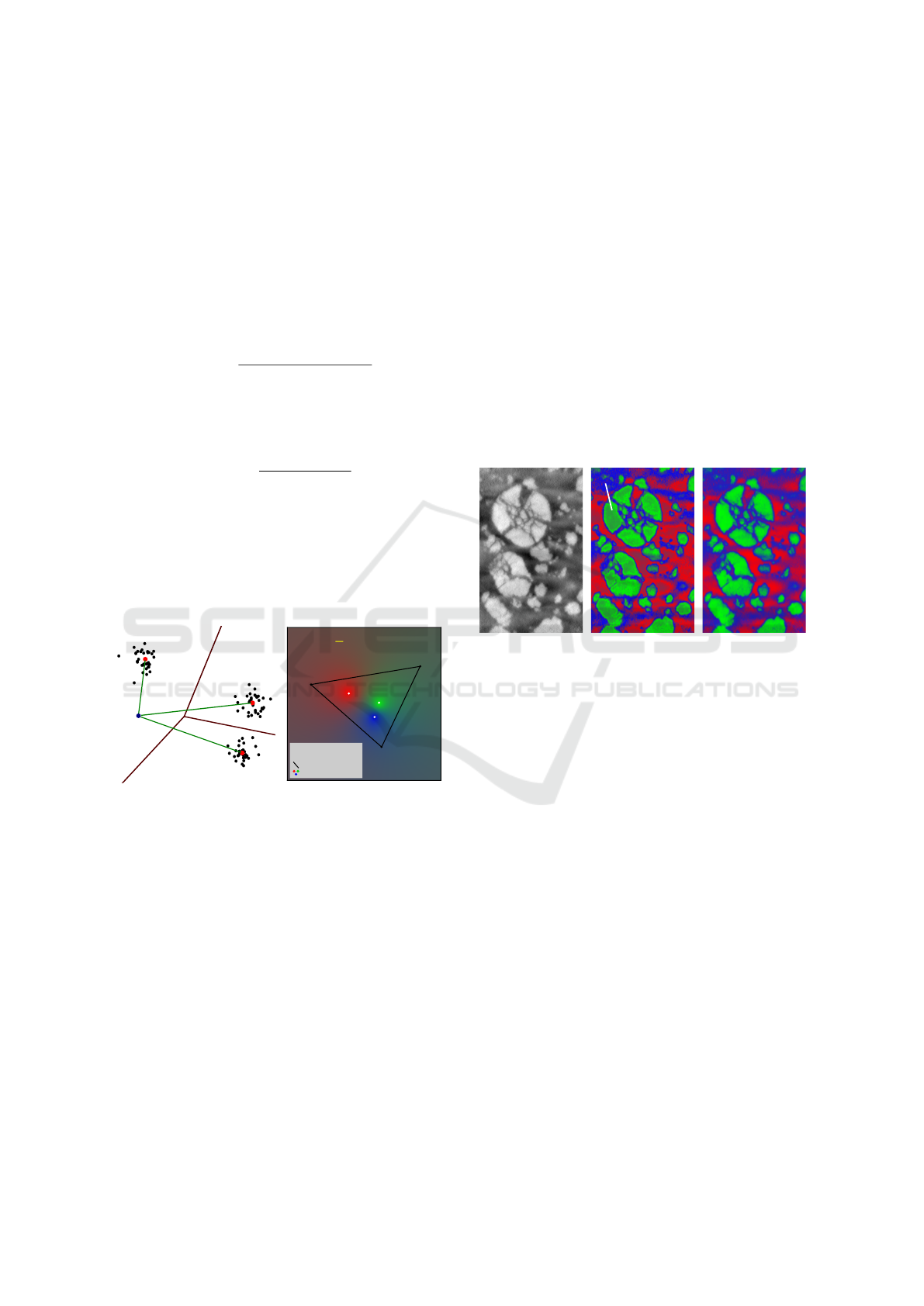
Figure 1: The distances to clusters’ centers given by the k-
means algorithm (1a) are used to compute density functions
(color map in 1b) using Eq.3: endmembers have lower den-
sity values than the center of their corresponding class (1b).
Although these density functions are widely used
and appropriate in a context of classification only, one
major issue is that they are not compatible with the
endmember-mixture modelling (Eq.1):
• the presented distance-based density functions
give a higher value to points close to the centers
(means) of the clusters than to any further point ;
thus, as the data is inside a simplex for which the
vertices represent the endmembers, these last ones
will have a lower density value than the centers
computed by any clustering algorithm (Fig.1,1b) ;
• the Gaussian mixture function and the Maha-
lanobis distance-based approach (the GMM mod-
elling alone) do not guarantee path-connected
class subsets ; therefore, two different endmem-
bers of the simplex could be associated with the
same class (or at least have close density vectors).
The same observations can be made for the other
usual density functions associated with clustering al-
gorithms, such as the Fuzzy C-means or any other
functions based on the distance to clusters or to their
centers. One consequence of such density functions
is that “holes” appear in density maps: in Fig.2 here-
inafter, as the centers of clusters are not located on
the extreme spectral values, the usual density func-
tions assign a lower probability value to the brightest
pixels than to pixels closer to the center of the class,
regarding the brightest class (cracking particles).
(a) Original image.
>
hole
(b) Computed map. (c) Expected map.
Figure 2: Grayscale image from the first band of a 4-band
spectral image of a Li-ion battery (2a), and probability map
computed with Eq.3 on 3 k-means centroids (2b) to seg-
ment three chemical phases (high, medium and low values
in 2a): the density function creates holes in the probability
map compared to the expected one (2c) ; see green phase.
We thus need to define a density function which
guarantees path-connected classes, such that the more
a point is “deep” inside its class (or “far” from the oth-
ers), the highest density value it will be assigned to.
This way, with an adapted classifier, the endmembers
(and close points) will have the highest density values,
and contrasts inside the classes will be preserved.
2.2 Proposed Approach
The idea of the proposed approach is quite simple: in-
stead of taking distances to clusters (or their centers),
we will consider signed distances to the classes’ fron-
tiers. Moreover, if the data is suitable, to guarantee
that the classes are path-connected, and to make the
structure more harmonious and the interpretation eas-
ier, we will consider here linear classifiers only.
By definition of linear classifiers, frontier hyper-
planes are built to separate the classes, which are then
ICPRAM 2025 - 14th International Conference on Pattern Recognition Applications and Methods
194

represented by distinct and complementary convex n-
dimensional polyhedra in the Euclidean space R
n
. We
thus consider the two following classifiers:
• the k-means clustering algorithm, for which the
classes are defined by the Voronoi cells (Fig.3) ;
• the application of a GMM on the unlabelled data,
followed by a SVM on the labelling given by the
GMM to fit frontier hyperplanes between classes.
The first method is better adapted to isotropic
Gaussian distributions with the same covariance ma-
trix, the second one for anisotropic Gaussian distri-
butions with different covariance matrices (more gen-
eral). Other classifiers can obviously be used as long
as they give polyhedral classes as results.
The signed Euclidean distance between the mea-
sured point x ∈ R
n
and each of the k polyhedral
classes P ⊆ R
n
is then computed, resulting in a vec-
tor of k signed distances associated with x, before ap-
plying the softmax function of the opposite distances
(Eq.2) to obtain its corresponding density vector.
1
C
3
C
2
C
Voronoi
frontiers
x
<
<
<
d
3
d
2
d
1
(a) Sgn-distance to frontiers.
P (e ) 1
-
~
11
1
C
1
e
2
e
3
e
3
C
2
C
e
C
: cluster centroid
: endmember
: simplex edge
: density function
(b) Density functions.
Figure 3: The signed distances to clusters’ frontiers given
by the k-means algo. (3a) are used to compute density func-
tions (3b) using Eq.2: endmembers have higher density val-
ues than the center of their corresponding class (3b).
Figure 3 shows how this simple approach ad-
dresses the limits of existing density functions high-
lighted in the previous section: points which are the
deepest ones in their respective class have the highest
density values. If the true endmembers are not given,
we can assume that, regarding the linear segmenta-
tion made, they are the most likely to be located in
space where probabilities are the highest. Unlike reg-
ular approaches, it allows furthermore preserving the
contrasts of segmented phases in the original spectral
image inside their respective classes (Fig.2c).
Although the distance from a point in the Eu-
clidean space to a convex polyhedron is easy to repre-
sent, computing it turns out to be a challenging task.
In the following sections, we formulate the problem
mathematically, review the different approaches in the
literature, and highlight the problems raised by the ex-
isting methods. We propose in this paper a mathemat-
ical process allowing computing the exact minimum-
norm point to any convex polyhedron, which, despite
of having an exponential complexity in the worst case
along the number k of support hyperplanes of the
polyhedron (iif n > 2), turns out to be fast in practice
for one to thirty hyperplanes.
3 DISTANCE TO CONVEX
POLYHEDRA: PROBLEM
FORMULATION
3.1 Definitions and Mathematical
Formulation
We work here in the Euclidean space R
n
of finite di-
mension n ∈ N
∗
with inner product ⟨·, ·⟩. To each of
the k (affine) hyperplanes H ⊆ R
n
given by any lin-
ear classifier, is associated one unique scalar-vector
couple (s, v) ∈ R × R
n
, where v is the normed vector
orthogonal to H and s the distance of H to the zero
point 0
n
signed by direction v, such that
H = {x ∈ R
n
| ⟨x,v⟩ = s}. (4)
As v is unique, H is oriented. Such an hyperplane H
is the frontier of a unique closed (affine) halfspace B
“behind” H regarding v such that
B = {x ∈ R
n
| ⟨x,v⟩ ≤ s}. (5)
We write H
(s,v)
(resp. B
(s,v)
) the hyperplane defined
by Eq.4 (resp. halfspace defined by Eq.5) regarding
(s,v). Polyhedra can then be properly defined.
Definition 1 (Polyhedron). A subset P ∈ R
n
is a (con-
vex) polyhedron if it is the intersection of a finite num-
ber of closed halfspaces. It can be either bounded or
unbounded. A bounded polyhedron is called polytope.
(Bruns and Gubeladze, 2009)
Let h ∈ F (I,R×R
n
) be a family of k scalar-vector
couples h
i
= (s
i
,v
i
) ∈ R × R
n
indexed by I = J1,kK.
We write P
h
the polyhedron defined as follows
P
h
=
\
i∈I
B
h
i
. (6)
Figure 4 hereinafter allows us to better visualize this.
This representation of a convex polyhedron as the
intersection of closed halfspaces (Eq.6) is called a H-
representation (Gr
¨
unbaum et al., 1967). Alternatively,
Euclidean Distance to Convex Polyhedra and Application to Class Representation in Spectral Images
195

0 200 400 600 800
0
0
0
0
0
h
P
<
H
2
v
2
H
3
v
3
H
1
v
1
<
<
(a) A polyhedron.
0 200 400 600 800
0
0
0
0
0
h
P
<
H
2
v
2
H
3
v
3
H
1
v
1
<
<
(b) A polytope (bounded).
Figure 4: Example of an unbounded polyhedron (4a) and of
a bounded one (4b) formed by three closed halfspaces.
but for polytopes only, polyhedra can be represented
as the convex hull of a finite set of points in R
n
, which
are its vertices. This less general representation is
called the V -representation of a polyhedron.
The distance function d between two points x,y ∈
R
n
is the usual Euclidean distance: d(x,y) = ∥x −y∥
2
.
The distance between a point x ∈ R
n
and a subset S of
R
n
is then defined as
d : R
n
× P (R
n
) → R
+
x , S 7→ inf
y∈S
∥x − y∥
2
. (7)
Definition 2 (Minimum-norm point). A point y in the
subset S ⊆ R
n
minimizing the Euclidean distance to
x ∈ R
n
is called a minimum-norm point in S from x.
If S is convex, then the minimum-norm point y ∈ S
from the fixed point x ∈ R
n
is unique.
The challenge here is, given h ∈ F (I,R × R
n
), to
find a way of determining the minimum-norm point in
the convex polyhedron P
h
⊆ R
n
from any x ∈ R
n
. This
problem is also known in the literature as the near-
est point problem in a polyhedral set (Liu and Fathi,
2012). If x ∈ P
h
- which can be easily verified by
checking if max
i∈I
{⟨x,v
i
⟩ − s
i
} is non-positive -, then
the nearest point in P
h
is x itself.
As we are looking for the signed distance from x
to the polyhedron’s frontiers ∂P
h
in the objective of
computing our proposed density function using Eq.2,
we define the usual signed distance function d
s
be-
tween a point x ∈ R
n
and a subset S of R
n
as
d
s
: R
n
× P (R
n
) → R
x , S 7→ sgn(1
x /∈S
−
1
2
) × d(x, ∂S)
. (8)
If x ∈ P
h
, then its signed distance to the frontiers
of P
h
is its distance to the complementary P
∁
h
of P
h
in
R
n
put to the negative ; otherwise, it is the distance to
the polyhedron itself. In this first case, d
s
(Eq.8) can
be easily put under an explicit formula: ∀x ∈ P
h
,
d
s
(x,P
h
) = max
i∈I
⟨x,v
i
⟩ − s
i
∥v
i
∥
2
. (9)
In the second case (x /∈ P
h
), where the signed distance
d
s
to P
h
is the Euclidean distance d to P
h
, there is un-
fortunately no explicit usable formula for the general
case. Bergthaller and Singer managed to give an ex-
act expression of the solution, but which uses unde-
termined parameters (Bergthaller and Singer, 1992).
To compute it, we need an algorithmic approach.
In the next section, we review the different possible
approaches and the state-of-the-art algorithms, and
show their limits from a mathematical point of view.
3.2 Existing Algorithms and Their
Limits
In the literature, most of the methods designed to
solve the nearest point problem in a polyhedral set are
geometric-based approaches, where a polyhedron P is
seen as a geometrical structure in space, defined either
by its vertices (V -representation) or by its support hy-
perplanes (H-representation), and where the problem
is solved using projection-based algorithms.
Equivalently, in H-representation, we can con-
sider this problem as a convex quadratic program-
ming problem, where P is the set of all solutions y
to the linear matrix inequality V.y ≤ S, with V the ma-
trix of all the v
i
and s the vector of all the s
i
, in the
space centered on the reference x ∈ R
n
, and where the
minimum-norm point is given as a solution to
Minimize ∥z∥
2
2
Subject to V z ≤ s
. (10)
Among the classical methods, Wolfe’s algorithm
(Wolfe, 1976) and Fujishige’s dual algorithm (Fu-
jishige and Zhan, 1990) remain popular processes for
finding the minimum-norm point in a convex poly-
tope. Several other algorithms have been developed
for the three-dimensional case only (Dyllong et al.,
1999), which is too restrictive for our problem.
Most of the methods that use H-representation
only consider the convex quadratic programming
problem (10) solved using conventional algorithms,
such as the simplex method (Wolfe, 1959), interior
point methods (Goldfarb and Liu, 1990), successive
projection methods (Ruggiero and Zanni, 2000), or
the Frank-Wolfe algorithm (Frank et al., 1956).
Recent algorithms either revisit these classical
methods (Jaggi, 2013), are based on complex ob-
jects that require a relatively large amount of com-
putational effort (Liu and Fathi, 2012), or are based
on a gradient descent such as the Operator Splitting
Quadratic Program (OSQP) (Stellato et al., 2020).
ICPRAM 2025 - 14th International Conference on Pattern Recognition Applications and Methods
196

Regardless of the approach, the known methods
can be classified into two main categories:
• the ones which guarantee to give the exact solu-
tion to the problem in a finite number of iterations
(Wolfe, Fujishige, Dyllong, etc.) ;
• the ones which give, unless in particular cases, an
approximation of the solution only, based on an
iterative algorithm converging to the optimal so-
lution when the number of iterations tends to in-
finity (Frank-Wolfe, Interior Point, OSQP, etc.).
In our case, even though it is not a necessary
requirement, we will focus on exact methods only.
Moreover, as the distance must be computed for all
the pixels in our spectral images and to each of the
polyhedral classes, we need to run the algorithm thou-
sands to millions of times depending on the size of
the image: we therefore need a fast and light algo-
rithm for our practical case, i.e. where polyhedra are
defined by a small or medium number of hyperplanes.
Most of the exact methods are based on the ver-
tices, which is critical for us, as linear classifiers usu-
ally return the family h of the couples (s, v) describing
separation hyperplanes between polyhedral classes
(H-representation), and as there necessarily are un-
bounded polyhedra in the resulting segmented space.
Converting a polyhedron into its V -representation is
computationally expensive, as we have first to verify
that it is unbounded (k ≥ n), then to find all its ver-
tices, resulting in

k
n

equations to solve (Saaty, 1955).
We therefore developed a geometric-based algo-
rithm which uses some mathematical properties of
polyhedral sets to optimize the iterative research of
the minimum-norm point, and which is fast in practice
for a small to medium number of hyperplanes defin-
ing the polyhedron (one to thirty). In the next section,
we’ll present the properties on which relies the algo-
rithm and its main lines.
4 AN EXACT MIN-NORM POINT
CALCULATION PROCESS FOR
CONVEX POLYHEDRA
4.1 Support Hyperplanes and
Minimum H-Description
Before getting started with the algorithm and its prop-
erties, we will first simplify the problem. If the set
of the halfspaces defining a polyhedron P in its H-
representation has not been processed yet - which is
the case for the linear classifiers used in this work -,
there may exist halfspaces which have no impact on
the construction of P, i.e. for which their removal
from the intersection (Eq.6) does not change set P.
The objective of this subsection is to find a way of de-
tecting all these “unnecessary” halfspaces to remove
them from the intersection, to make P lighter and have
better performances on the proposed algorithm.
Definition 3 (Support Hyperplane). Let H ⊆ R
n
be an
affine hyperplane. If the polyhedron P is contained in
one of the two closed halfspaces bounded by H, then
H is called support hyperplane of P if P ∩ H ̸=
/
0.
With such definition (3) given in (Bruns and
Gubeladze, 2009), we can easily understand that all
the halfspaces whose frontier hyperplane is not a sup-
port hyperplane of P are unnecessary for the defini-
tion of P. In Figure 5 hereinafter, H
4
is not a support
hyperplane of P: the corresponding halfspace is there-
fore removed from the intersection defining P.
0 200 400 600 800
0
0
0
0
0
H
2
v
2
<
H
4
v
4
<
<
H
1
H
5
v
1
v
5
<
H
3
v
3
<
h
P
(a) A polyhedron.
0 200 400 600 800
0
0
0
0
0
H
2
v
2
<
H
1
v
1
<
H
3
v
3
<
h
P
(b) Its min H-description.
Figure 5: Example of a polyhedron (5a) as the intersec-
tion of five halfspaces, and its minimum H-description (5b)
where only the three first halfspaces have been preserved.
Verifying P ∩ H ̸=
/
0 for all hyperplanes H of the
description of a polyhedron P is very simple and al-
lows removing part of the unnecessary halfspaces.
But the condition of being support hyperplanes is ac-
tually not sufficient to remove all the unnecessary
halfspaces to obtain what we call the “minimum H-
description” (4) of P (Gr
¨
unbaum et al., 1967): in
Fig.5a, H
5
is a support hyperplane as it “touches” one
of the polyhedron’s vertices, but is not necessary, be-
cause, if we remove its associated halfspace from the
intersection, P does not change. We thus need a more
powerful filtering condition on halfspaces.
Definition 4 (Minimum H-description). Let B =
(B
1
,B
2
,...,B
k
) be a family of k closed halfspaces,
and let P =
T
i∈I
B
i
. We call minimum H-description
of P a subfamily B
′
of B with k
′
elements, such that
T
i∈I
′
B
′
i
= P and ∀ j ∈ I
′
,
T
i∈I
′
\{ j}
B
′
i
̸= P.
Note that if P is full-dimensional (i.e. of dimension
n), then its minimum H-description is unique.
Euclidean Distance to Convex Polyhedra and Application to Class Representation in Spectral Images
197

From this definition (4) comes the following
proposition, which allows directly verifying if an half-
space B
j
in the description of P is in its minimum H-
description (thus is necessary) or not.
Proposition 1. The minimum H-description of the
polyhedron P is the family of all halfspaces B
j
in B
such that B
∁
j
∩

T
i∈I\{ j}
B
o
i

̸=
/
0.
B
∁
being the complement of B in R
n
, B
o
its interior.
As the condition in Proposition 1 uses open sets
only (complement and interior of a closed set), it can
be easily expressed by a condition on a strict linear
matrix inequality, with j ∈ I, as follows
∃x ∈ R
n
, A
j
x < b
j
(11)
with the matrix A
j
= (v
1
,...,v
j−1
,−v
j
,v
j+1
,...,v
k
)
⊺
and the vector b
j
= (s
1
,...,s
j−1
,−s
j
,s
j+1
,...,s
k
)
⊺
.
The condition in Proposition 1 is equivalent to ver-
ifying the consistency of the matrix inequality in (11).
To do so, regular approaches can be used, such as lin-
ear programming with the zero function to minimize
subject to the constraints (11), or the I-rank of the sys-
tem for small dimensions of A
j
(Dines, 1919). This
way, each time we’ll need to, we can easily get the
minimum H-description of any polyhedron P.
4.2 Preliminary Algorithm
The main algorithm which allows computing the ex-
act minimum-norm point in any polyhedral set P is
based on successive projections of the reference x on
methodically-chosen support hyperplanes of P until
the minimum-norm point is reached.
To better understand its main steps and the prop-
erties it uses, we will first introduce a preliminary al-
gorithm A
1
(1), which allows projecting the reference
point x ∈ R
n
on an intersection of hyperplanes.
From any x ∈ R
n
and any h ∈ F (I,R × R
n
) for
which the v
i
are linearly independent, algorithm A
1
successively projects x on all the hyperplanes formed
by couples (s
i
,v
i
) in h in the order given by I. At each
iteration i ∈ I, with the aim of projecting x on the i-
th hyperplane, the projection direction w
i
is computed
from v
i
by removing from it all its components ⟨v
i
,u⟩u
in the space formed by the set of previous projection
directions U. This way, by moving x at iteration i in
direction w
i
(which is non-zero, as the v
i
are linearly
independent), the point will always stay in the hyper-
planes considered in previous iterations j < i, as w
i
is orthogonal to all the previous v
j
by construction.
Then, w
i
is normed, resulting in u
i
, and the projection
distance d
i
is computed such that moving x in direc-
tion u
i
with a distance d
i
will allow the new x being
Algorithm 1: Projection on intersection of hyperplanes.
Data: · x ∈ R
n
· h ∈ F (I, R × R
n
)
such that (v
i
)
i∈I
is linearly independent
Result: y ∈ R
n
such that y ∈ ∩
i∈I
H
i
y ← x;
U ←
/
0;
for i ∈ I do
w
i
← v
i
−
∑
u∈U
⟨v
i
,u⟩u;
u
i
←
w
i
∥w
i
∥
;
d
i
←
⟨x,v
i
⟩−s
i
⟨u
i
,v
i
⟩
;
y ← y − d
i
u
i
;
U ← U ∪{u
i
};
end
in the i-th hyperplane. u
i
is then added to U before
going to the next iteration. Note that U is formed by
the Gram-Schmidt process on the family (v
i
)
i∈I
.
This simple algorithm has fundamental properties
which will be used for the main algorithm. Let’s now
consider any family h ∈ F (I, R × R
n
) of k scalar-
vector couples h
i
= (s
i
,v
i
) ∈ R ×R
n
indexed by I. We
have the following proposition.
Proposition 2. Let h
∗
be a subfamily of h such that
the v
∗
i
are linearly independent. Then, the result of A
1
y = A
1
(x,h) is the minimum-norm point in the inter-
section ∩
i∈I
∗
H
∗
i
of hyperplanes formed by h
∗
from x.
As it is obvious that, if x /∈ P
h
, there exist at least
one support hyperplane of P
h
such that the minimum-
norm point in P
h
from x is in this hyperplane, from
Proposition 2 directly comes the following corollary.
Corollary 1. There exists a subfamily h
†
of h such
that A
1
(x,h
†
) is the min-norm point in P
h
from x.
Writing h
′
the subfamily of all the couples h
i
of h
whose hyperplane H
h
i
contains the minimum-norm
point in P
h
from x, h
†
is more precisely any subfamily
of h
′
such that (v
i
)
i∈I
†
is a basis of span((v
i
)
i∈I
′
), with
I
†
the indices on h
†
and I
′
the ones on h
′
.
With Corollary 1, we are facing the one problem:
how may we determine such a subfamily h
†
? Before
this, how may we determine h
′
, i.e. the family of the
hyperplanes containing the minimum-norm point?
As we know, such subfamilies are actually hard
to determine without having any information on the
polyhedron’s vertices, or without using complex and
computationally-expensive structures (Liu and Fathi,
2012). Our method consists then in modifying algo-
rithm A
1
to search the minimum-norm point in P
h
by
recursively projecting x on all the possible hyperplane
combinations, until the min-norm point is reached.
ICPRAM 2025 - 14th International Conference on Pattern Recognition Applications and Methods
198

4.3 Main Algorithm
As the number of hyperplane combinations is an ex-
ponential function of the number k of support hyper-
planes of P
h
(2
k
), we then need a methodical search:
we want to avoid unnecessary combinations, and start
the search with the hyperplanes that are the most
likely to contain the minimum-norm point.
The first thing that we modify in A
1
is the addition
of dimension reduction at each iteration: as, from it-
eration i to i + 1, the new direction vector u
i+1
and
the new distance of projection d
i+1
are built such that
x stays in the hyperplanes previously considered, we
will, each time we go “deeper” in the projections from
i to i + 1, instead of considering the problem in R
n
,
consider it in the affine subspace of lower dimension
formed by the hyperplane H
h
i
on which has just been
projected x, and transform the family h into a new one
h
′
which is expressed in this new subspace as follows
∀ j ∈ I \ {i},





v
′
j
=
v
j
−⟨v
j
,v
i
⟩v
i
/∥v
i
∥
2
2
∥
v
j
−⟨v
j
,v
i
⟩v
i
/∥v
i
∥
2
2
∥
2
s
′
j
= ⟨x,v
′
j
⟩ −
⟨x,v
j
⟩−s
j
⟨v
j
,v
′
j
⟩
. (12)
This way, at each new iteration i + 1, after reduc-
ing space dimension and the family h into h
′
using
Eq.12, the new direction vector u
′
i+1
will simply be
v
′
i
/∥v
′
i
∥
2
, and the distance of projection d
′
i+1
will be
the signed distance from x to the halfspace B
h
′
i+1
, ex-
actly as it is at iteration 1 when U is empty.
This space reduction does not only allow working
in a reduced space R
n−i
at iteration i + 1, but it also
allows generalizing properties that can be made at it-
eration 1 on h to all the following iterations i + 1 on
the modified h
′
. Which is crucial for the following
properties that will be used for the main algorithm.
Proposition 3. There exists a couple (s,v) in h such
that the signed distance d
s
between x and the half-
space B
(s,v)
is positive, and its frontier hyperplane
H
(s,v)
contains the minimum-norm point in P
h
from x.
Proposition 4. If there exists a couple (s,v) in h such
that the projection x −
d
s
(x,B
(s,v)
)
∥v∥
2
v of x on the hyper-
plane H
(s,v)
is in P
h
, then the signed distance d
s
be-
tween x and B
(s,v)
is the maximum of the signed dis-
tances d
s
from x to all the halfspaces defined by the
couples in h, i.e.: d
s
(x,B
(s,v)
) = max
i∈I
d
s
(x,B
(s
i
,v
i
)
).
Proposition 5. If n ≤ 2 and h describes the min H-
description of P
h
, then the min-norm point in P
h
from
x is in the hyperplane of maximum (positive) distance
to x, i.e. in H
(s
i
,v
i
)
where i = argmax
i∈I
d(x,B
(s
i
,v
i
)
).
Note that the reciprocals of Prop. 4 and 5 are false.
Criterion 1. The point y ∈ P
h
is the minimum-norm
point in P
h
from x if and only if P
o
h
∩B
o
(s
∗
,v
∗
)
=
/
0 , with
s
∗
= ⟨y, y − x⟩ and v
∗
= y − x.
Criterion 1 allows verifying if a point y in P
h
is the
min-norm point from x, and is equivalent to the con-
sistency of a strict linear matrix inequality like (11).
The main algorithm is a recursive algorithm which
can either go “deeper” in the projection process of
x considering allowed-to-project hyperplanes, or go
back in a previous state of x if deeper projections are
not possible or unnecessary at the current recursion.
At the beginning of each recursion, we consider the
whole original family h, which is then filtered, trans-
formed and sorted using the propositions seen before.
At the end of the recursion, the algorithm enters a
loop over the filtered h
i
in which x is projected on
H
h
i
and then put in a deeper recursion step. This way,
x can be projected on all the possible combinations of
hyperplanes, but which are methodically filtered and
sorted, until the minimum-norm point is reached.
Each recursion then follows these main lines:
1. if x is the minimum-norm point in P
h
(Criterion
1), then stop and return x ; otherwise, continue ;
2. if x ∈ P
h
but is not the minimum-norm point, then
go back in the previous recursion ;
3. transform h into the reduced h
′
using Eq.12 ;
4. filter h
′
:
• remove from h
′
the h
′
i
whose v
′
i
is linearly de-
pendant of U (set of orthonorm. projection vec-
tors from previous recursions) for Corollary 1 ;
• remove from h
′
the h
′
i
for which d
s
(x,B
h
i
) ≤ 0
(Prop. 3) ;
• compute the minimum H-description of P
h
′
(useless h
′
i
are removed from h
′
) using Eq.11;
5. if the filtered h
′
is empty, go back in the previous
recursion ;
6. sort h
′
from the greatest distance d
s
(x,B
h
′
i
) to the
smallest, to increase the chances of projecting first
on a hyperplane containing the minimum-norm
point (Prop. 4 and 5) ;
7. in a loop, for h
′
i
in h
′
:
• project x on H
h
′
i
;
• definitely remove h
′
i
from h
′
for the deepest re-
cursions and the following iterations in the loop
(it avoids permutations) ;
• call the function with these new parameters ;
• if the minimum-norm point has not been found,
put back x in its previous state ;
8. if the minimum-norm point has not been found
yet, go back in the previous recursion ;
Euclidean Distance to Convex Polyhedra and Application to Class Representation in Spectral Images
199

4.4 Comparison with a State-of-the-Art
Algorithm
Built this way, our algorithm ensures to return the ex-
act solution to the nearest point problem in a polyhe-
dron P, in a finite number of steps. However, even if
the search of the minimum-norm point is optimized
by mathematical properties developed in the previous
subsections, its complexity in the worst case is expo-
nential, in O(2
k
) times a polynomial expression of k,
with k the number of support hyperplanes of P.
To evaluate its complexity in time over the num-
ber k in practical case, we implemented it in the C
programming language, and built a stochastic model
which generates polyhedra with a given number k of
support hyperplanes in dimension n. We then chose
to compare the performances of our algorithm to one
of the most recent methods able to rapidly solve con-
vex quadratic problems such as ours: the OSQP solver
(Stellato et al., 2020). This solver is based on an
automatically-optimized gradient descent, and com-
putes an approximation of the solution point.
The two following figures are the results of two
experiences: in the first one (6), we fixed n = 3 to
study the performances of the algorithms in the 3-
dimensional Euclidean space ; in the second one (7),
we let n = k (as, in spectral images, the number of
bands, n, is usually greater than the number of classes
or endmembers, ≥ k + 1). Both graphs represent the
evolution of computation time over the number k.
The blue discontinuous curve representing the OSQP
solver, with a given relative tolerance of 10
−6
, and the
green continuous one representing our method. For
every k, the computation time values are the means of
1000 simulations with different polyhedra.
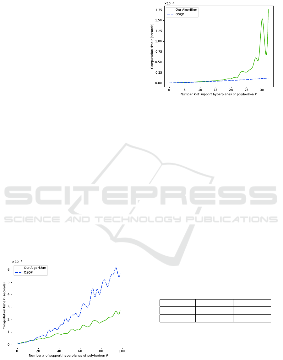
Figure 6: Evolution of computation time t over the number
k of support hyperplanes (averaged over 1000 simulations
per value of k), for the OSQP solver (blue) and our algo-
rithm (green), in dimension n = 3.
Figure 7: Evolution of computation time t over the number
k of support hyperplanes (averaged over 1000 simulations
per value of k), for the OSQP solver (blue) and our algo-
rithm (green), in dimension n = k.
Figure 6 reveals that, when n is fixed and relatively
small (n = 3), our method has similar or even bet-
ter performances than the OSQP solver, and this for
all values of k. It moreover seems that, the greater k
is, the more significant the difference between OSQP
and our algorithm is. The expected exponential be-
haviour of our method actually appears here to be al-
most linear or polynomial, from k = 1 to k = 100.
On the other hand, Figure 7 highlights a way dif-
ferent behaviour of our algorithm when n follows k:
its associated computation time stays equivalent to
the OSQP’s one from k = 1 to around k = 15 or 20,
but becomes exponential over k after k = 20 and ex-
plodes around k = 30. This shows that our algorithm
is limited when we need to consider more than 30 sup-
port hyperplanes in higher dimensions. In practice, as
we use it for our density function in cases where the
number of considered classes rarely exceeds twenty
or thirty, this behaviour will not be a problem for us.
Table 1: Mean and standard deviation of the distance be-
tween the point computed by the OSQP solver and the exact
point from our method (over all the K × 1000 simulations).
Experience n = 3 n = k
Mean error 9.87 × 10
−3
6.31 × 10
−4
STD 1.08 × 10
−2
3.80 × 10
−4
As our method gives the exact solution and OSQP
an approximation, one last thing to analyse is the
mean distance between the point given by OSQP and
the one by our method. Table 1 shows that the mean
error made by OSQP and the standard deviation are
both higher in the case where n = 3 than where n = k.
In both cases, most of the distances are between 10
−4
and 10
−1
(sometimes greater when n = 3), which may
be not convenient if we look for a high precision.
ICPRAM 2025 - 14th International Conference on Pattern Recognition Applications and Methods
200

5 APPLICATION TO CLASS
REPRESENTATION
5.1 Abundance Map Estimation
In this section, to evaluate the performances of our ap-
proach, we apply it to one of the most widely used hy-
perspectral datasets for hyperspectral unmixing: the
Samson dataset. Typically well suited to the linear
endmember-mixture modelling, it is composed of 156
bands and represents 3 regional classes: water, forest
and soil. We chose here the use of a GMM followed
by a SVM to segment space into polyhedral subsets.
We then computed for each pixel x its signed distance
to each of the polyhedra using our algorithm.
In this subsection, the idea is to find back the abun-
dance map (A in Eq.1) from estimated endmembers
(M). To do so, like most of the approaches for spec-
tral unmixing, we assume that, among the observed
data, there exist some spectra close enough to the real
endmembers. We use our method to determine these
endmembers by taking, in each class, the spectrum
which is the “deepest” one in the corresponding poly-
hedron, i.e. which has the lowest signed distance: it
should represent the purest class spectrum. We classi-
cally reduce and inverse the resulting matrix M of the
endmembers, to then compute the abundance map A.
0 20 40 60 80
0
20
40
60
80
marcouille
0.0
0.2
0.4
0.6
0.8
1.0
Soil Tree Water
Estimated Ground Truth
Figure 8: Ground truth (1st row) and estimated abundance
maps (2nd row), for the three classes (columns) of Samson.
The Root Mean Squared Error (RMSE) is about 0.1533.
Figure 8 shows the abundance maps of the three
classes given by our method (second row) compared
to the ground truth (first row). To evaluate the qual-
ity of these results, we compare them to state-of-the-
art methods among the most effective ones for hy-
perspectral unmixing: a geometric distance-based ap-
proach like ours, the new maximum-distance anal-
ysis (NMDA) from (Tao et al., 2021) ; and a deep
learning approach, the spatial–spectral adaptive non-
linear unmixing network (SSANU-Net) from (Chen
et al., 2023). We computed the RMSE between our
results and the ground truth, and compared it to the
best RMSE of the abundances given in these papers.
Table 2: RMSE of the abundance maps given by the three
considered methods on the Samson dataset, and processing
time (for ours, RMSE and time are the means on 100 runs).
Method NMDA SSANU-Net Ours
RMSE(A) 0.1620 0.1668 0.1533
time (s) 1.4743 unknown 1.9697
Table 2 shows that our method has better perfor-
mances than the two others regarding the RMSE of
the abundance map A. As our method depends on a
probabilistic model (GMM), we averaged the RMSE
and the computation time on 100 independent runs,
using a ratio of 0.2 for the random sample extraction
for the training of the GMM. These results given by
our method seem quite stable, as the standard devia-
tion of the RMSE on all the runs is about 0.0061.
The computation time (tab.2) of our method is
however greater than the NMDA’s one, but is the re-
sult of the addition of the training time of the GMM,
the fitting time of the SVM, and the computation time
of the distances to polyhedra given by our algorithm.
Taken separately, the mean computation time of our
algorithm for all the pixels in the image and all the
polyhedral subsets is about 0.06 seconds only. Al-
though these results are good, we have to remind that
they highly depend on the linear classifier chosen.
5.2 Probability Map Calculation
We consider here the more general case, where we
don’t know whether the linear endmember-mixture
modelling (Eq.1) is suitable to the spectral image or
not. In this case, there is no search for endmembers or
for linear combinations of them in the observed data:
we simply use a given density function on the seg-
mentation of the space made by a chosen classifier.
We then only use here the softmax function (Eq.2)
of the opposite signed distances to polyhedral classes
divided by their standard deviation. If the classes are
not homogeneously shared in the spectral space - like
in Samson’s -, a change of basis can be made in the
space of signed-distance vectors, using the vectors of
lowest distance value for each class as new basis.
The resulting density map is then, by construction,
more suitable to a probability map associated with
the segmentation made (by here our GMM and SVM
model). We want to show, with the Samson dataset,
that this general method gives good results even on
spectral datasets which are well suited to Eq.1.
Figure 9 reveals that this approach gives even a
Euclidean Distance to Convex Polyhedra and Application to Class Representation in Spectral Images
201

0 20 40 60 80
0
20
40
60
80
marcouille
0.0
0.2
0.4
0.6
0.8
1.0
Soil Tree Water
Estimated Ground Truth
Figure 9: Ground truth (1st row) and computed probability
maps (2nd row), for the three classes (columns) of Samson.
The Root Mean Squared Error (RMSE) is about 0.0985.
better estimation of the density maps on the Sam-
son dataset than any of the endmember-unmixing ap-
proaches in table 2: with the same parameters for the
GMM, the mean RMSE (still over 100 runs) between
the determined maps and the ground truth is 0.0985,
with a standard deviation of 0.0103, which represents
the best results in terms of RMSE among the ones
from our study and from the two papers taken as ref-
erence in this section, and probably one of the best in
the literature for Samson, regardless the approach.
5.3 Phase Extraction
In this last subsection, we want to validate our method
by applying it on a dataset of spectral images which
are clearly not suitable to the linear endmember-
mixing modelling. To this end, we study here a set
of spectral images of a Lithium-ion battery captured
by X-ray nano-CT under four spectral bands (or “en-
ergies”). Our work originally started with this dataset.
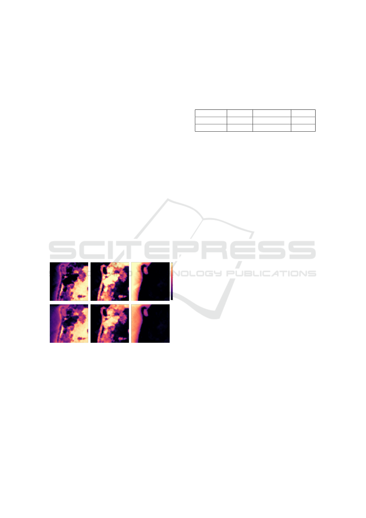
(a) Band 1. (b) Band 2. (c) Band 3. (d) Band 4.
Figure 10: Spectral image of a Lithium-ion battery captured
by tomography X with four bands (10a, 10b, 10c, 10d).
Figure 10 reveals how correlated the spectra of the
data are: a pixel which has a certain value on one of
the four bands is likely to have the same value on the
other bands. Which is incompatible with any linear
unmixing approach, as the data is distributed on one
line in the spectral space, making the possible end-
members linearly dependant (M not invertible).
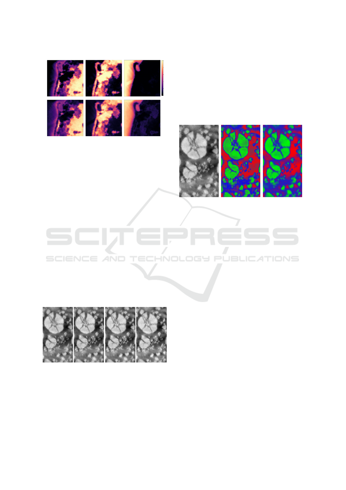
The objective is then to be able to extract the three
visible phases in these images (Fig.10): NMC parti-
cles (high values - green), CBD (blurry medium val-
ues - blue), and porosity (low values - red). These
phases will be represented by their probability map
determined by our general method previously seen,
but with a k-means as classifier instead of a GMM.
(a) Original image. (b) Usual prob map. (c) Our prob map.
Figure 11: Image of the first band of the Li-ion battery
dataset (11a), the usual probability map given by Eq.3 on
the distances to k-means centroids (11b), and the one given
by our approach with the same k-means parameters (11c):
our method allows preserving contrasts in the phases, unlike
the usual one in which holes are created (green phase).
Unfortunately, there is no ground truth for this
dataset to evaluate the results of our approach. But, in
addition to mathematical guarantees, visual results in
Fig.11 allow validating the fact that our method pre-
serves the contrasts (gradient) in probability maps in-
side the classes (11c). Which is not the case for usual
density functions (11b). The visually-coherent map
resulting from our approach validates its consistency
in spectral images which cannot be linearly unmixed.
6 CONCLUSIONS AND
PERSPECTIVES
With the aim of addressing the cases where spectral
images cannot be linearly unmixed, we developed a
new approach which allows building an adapted den-
sity map from observed data. Density functions usu-
ally used for clustering models suffer from limits in
the context of spectral unmixing: they are either based
on the distances to clusters, which does not allow de-
tecting any endmember and creates holes in density
maps, or do not guarantee crucial spatial properties.
The new density function that we formulated to
ICPRAM 2025 - 14th International Conference on Pattern Recognition Applications and Methods
202

address these limits is based on the idea of comput-
ing the signed distance to the frontiers of polyhedral
classes given by linear classifiers. We developed an
algorithm capable of computing the exact minimum-
norm point in any polyhedral subset. Despite its expo-
nential complexity in the worst case, it remains faster
than the recent OSQP solver (Stellato et al., 2020) in
dimension 3, and still finds the solution rapidly up to
30 support hyperplanes in high dimension.
The application of our approach to the Samson
dataset highlights a better estimation of the abundance
maps than geometric-based and deep learning-based
state-of-the-art approaches, whether in the context of
abundance map or of probability map. In this last
context, our method gives even much better results.
Moreover, the results on a spectral dataset of a Li-
ion battery, incompatible with linear unmixing ap-
proaches, validate its relevance in the general case.
Despite such valuable results, some limits still re-
main: our algorithm for the minimum-norm point has
an exponential behaviour in high dimension over 30
hyperplanes, which is not desirable in practice for a
great number of classes. Furthermore, testing the ap-
proach on other datasets, compatible with linear un-
mixing approaches or not, such as the Cuprite dataset
(Tao et al., 2021), would bolster the observations and
conclusions made on the studied datasets.
To go further, although we have focused solely
on linear classifiers, we could extend our approach to
non-linear methods by applying it in a space of higher
dimension (feature map) given by a chosen mapping
function, compute the minimum-norm points to poly-
hedral classes in it, before going back to the original
space where classes and distances are non-linear.
ACKNOWLEDGEMENTS
This work was supported by the French Agence Na-
tionale de la Recherche (ANR), project number ANR
22-CE42-0025.
REFERENCES
Bergthaller, C. and Singer, I. (1992). The distance to a
polyhedron. Linear Algebra and its Applications,
169:111–129.
Bruns, W. and Gubeladze, J. (2009). Polytopes, rings, and
K-theory. Springer Science & Business Media.
Chang, C.-L., Lo, S.-L., and Yu, S.-L. (2006). The parame-
ter optimization in the inverse distance method by ge-
netic algorithm for estimating precipitation. Environ-
mental monitoring and assessment, 117:145–155.
Chen, X., Zhang, X., Ren, M., Zhou, B., Feng, Z., and
Cheng, J. (2023). An improved hyperspectral unmix-
ing approach based on a spatial–spectral adaptive non-
linear unmixing network. IEEE JSTARS, 16:9680–
9696.
Dines, L. L. (1919). Systems of linear inequalities. Annals
of Mathematics, 20(3):191–199.
Dyllong, E., Luther, W., and Otten, W. (1999). An accurate
distance-calculation algorithm for convex polyhedra.
Reliable Computing, 5(3):241–253.
Eches, O., Dobigeon, N., Tourneret, J.-Y., and Snoussi, H.
(2011). Variational methods for spectral unmixing
of hyperspectral images. In 2011 IEEE International
Conference on Acoustics, Speech and Signal Process-
ing (ICASSP), pages 957–960. IEEE.
Figliuzzi, B., Velasco-Forero, S., Bilodeau, M., and An-
gulo, J. (2016). A bayesian approach to linear un-
mixing in the presence of highly mixed spectra. In
International Conference on Advanced Concepts for
Intelligent Vision Systems, pages 263–274. Springer.
Frank, M., Wolfe, P., et al. (1956). An algorithm for
quadratic programming. Naval research logistics
quarterly, 3(1-2):95–110.
Fujishige, S. and Zhan, P. (1990). A dual algorithm for find-
ing the minimum-norm point in a polytope. Journal
of the Operations Research, 33(2):188–195.
Goldfarb, D. and Liu, S. (1990). An O(n
3
L) primal in-
terior point algorithm for convex quadratic program-
ming. Mathematical programming, 49(1):325–340.
Gr
¨
unbaum, B., Klee, V., Perles, M. A., and Shephard, G. C.
(1967). Convex polytopes, volume 16. Springer.
Jaggi, M. (2013). Revisiting frank-wolfe: Projection-free
sparse convex optimization. In International confer-
ence on machine learning, pages 427–435. PMLR.
Liu, Z. and Fathi, Y. (2012). The nearest point problem
in a polyhedral set and its extensions. Computational
Optimization and Applications, 53:115–130.
Ruggiero, V. and Zanni, L. (2000). A modified projec-
tion algorithm for large strictly-convex quadratic pro-
grams. Journal of optimization theory and applica-
tions, 104:255–279.
Saaty, T. L. (1955). The number of vertices of a polyhedron.
American Mathematical Monthly, 62(5):326–331.
Stellato, B., Banjac, G., Goulart, P., Bemporad, A., and
Boyd, S. (2020). OSQP: an operator splitting solver
for quadratic programs. Mathematical Programming
Computation, 12(4):637–672.
Tao, X., Paoletti, M. E., Haut, J. M., Han, L., Ren, P., Plaza,
J., and Plaza, A. (2021). Endmember estimation from
hyperspectral images using geometric distances. IEEE
Geoscience and Remote Sensing Letters, 19:1–5.
Winter, M. E. (1999). N-findr: An algorithm for fast au-
tonomous spectral end-member determination in hy-
perspectral data. In Imaging spectrometry V, volume
3753, pages 266–275. SPIE.
Wolfe, P. (1959). The simplex method for quadratic pro-
gramming. Econometrica, 27(3):382–398.
Wolfe, P. (1976). Finding the nearest point in a polytope.
Mathematical Programming, 11:128–149.
Euclidean Distance to Convex Polyhedra and Application to Class Representation in Spectral Images
203