Greedy Brain Source Localization with Rank Constraints
Viviana Hernandez-Castañon, Steven Le Cam and Radu Ranta
CRAN, Univ. de Lorraine-CNRS, Nancy, F-54000, France
Keywords:
Sparse Source Localization, Greedy Algorithms, Stepwise Regression, Rank Constraints, EEG.
Abstract:
This paper introduces a new low rank matrix approximation model and a greedy algorithm from the iterative
regression family to solve it. Unlike the classical Orthogonal Matching Pursuit (OMP) or Orthogonal Least
Squares (OLS), the elements of the dictionary are not vectors but matrices. For reconstructing a measurement
matrix from this dictionary, the regression coefficients are thus matrices, constrained to be low (unit) rank. The
target application is the inverse problem in brain source estimation. On simulated data, the proposed algorithm
shows better performances than classical solutions used for solving the mentioned inverse problem.
1 INTRODUCTION
This work finds its initial motivation in the inverse
problem of brain source estimation from electrophys-
iological signals. It can be formulated as the more
general problem of a constrained low rank matrix
approximation: given a dictionary of matrices
¯
K
i
∈
R
m×q
,(q < m) and a data matrix X ∈ R
m×n
,(m < n),
find the rank 1 matrices
¯
J
i
∈ R
q×n
such as the
˜
X =
∑
i
¯
K
i
¯
J
i
approximates closely X. Before introducing
the details of this model and the greedy algorithm we
propose, we will briefly justify it by explaining its ap-
plication in neuroscience.
Macroscopic brain electrophysiological signals X
are recorded by sensors placed on the scalp (EEG),
on the cortex (ECoG) or implanted in the brain
(SEEG). The sources J
i
that generate the measure-
ments are neural populations modelled as electrical
current dipoles, characterized by their positions, ori-
entations and amplitudes (6 parameters per dipole).
All possible positions are given as a grid of points in-
side the discretized brain volume. The sensors are dis-
tant to the active sources and thus they record a sum of
propagated activities. The propagation is assumed to
be instantaneous at the frequencies of interest (below
1kHz) and at the distances between sources and sen-
sors (few cm) Logothethis et al. (2007); Ranta et al.
(2017). The forward problem expressing the recorded
potentials knowing the dipolar sources’ characteris-
tics and the propagation environment writes thus in
the linear form introduced above, where the gain
(lead-field) matrix K relating the dipolar sources J
to the measurements X is known and it embeds the
geometry and physical properties of the propagation
environment (head-model).
The inverse problem aims to estimate the dipo-
lar sources (positions, orientations and amplitudes)
responsible for the measured signals. This is an ill-
posed problem, mainly because of its dimensions:
usually, only a few dozens of sensors are available (at
most a few hundreds), while the possible source posi-
tions and orientations are far more numerous, depend-
ing on the numerical resolution of the head model.
Noise and spatial redundancy add to the difficulties of
the problem.
The literature on inverse problem solving in brain
electrophysiology is extremely vast. Several tech-
niques were proposed in the last 30 years (see e.g., the
reviews from Baillet et al. (2001); Michel et al.
(2004); He et al. (2011, 2018)). We are particularly
interested in this paper in sparse methods, which aim
to estimate a low number of sources explaining most
of the measured signals. Scanning methods such as
MUSIC and beamforming, and in particular the iter-
ative versions such as (T)RAP-MUSIC Mosher and
Leahy (1999); Mäkelä et al. (2018), yield naturally
sparse solutions. They can be seen as two-steps ap-
proaches: first, scan for the most plausible positions
and orientations (i.e., choose among the columns of
the gain matrix the ones most likely to project the
sources on the sensors) and second estimate the am-
plitudes minimizing the error between the actual mea-
surements and their modeled counterpart. By con-
struction (sparsity + minimization), they do not com-
pletely explain the data (unlike minimum norm type
solutions Dale and Sereno (1993); Hämäläinen and Il-
Hernandez-Castañon, V., Le Cam, S. and Ranta, R.
Greedy Brain Source Localization with Rank Constraints.
DOI: 10.5220/0013386600003911
Paper published under CC license (CC BY-NC-ND 4.0)
In Proceedings of the 18th Inter national Joint Conference on Biomedical Engineering Systems and Technologies (BIOSTEC 2025) - Volume 1, pages 819-826
ISBN: 978-989-758-731-3; ISSN: 2184-4305
Proceedings Copyright © 2025 by SCITEPRESS – Science and Technology Publications, Lda.
819

moniemi (1994); Pascual-Marqui (2007)). They nei-
ther impose a fixed orientation for the estimated dipo-
lar sources, i.e., the three Cartesian projections of the
dipole are allowed to vary independently in time.
This paper proposes a new greedy algorithm de-
rived from the family of step-wise regressions on a
given (forward) dictionary
1
. Unlike for its predeces-
sors, the regressors are not column vectors, but matri-
ces, representing 3D lead-field matrices associated to
each possible source position. Moreover, the regres-
sion coefficients for each source (time varying dipo-
lar amplitudes) are explicitly constrained to have es-
timated fixed orientations. Thus, compared to state-
of-the-art methods based on distributed source mod-
els where the source orientations are fixed and known
(e.g., Gramfort et al. (2013); Korats et al. (2016)),
the proposed method explicitly estimates sources with
fixed orientations starting from a freely oriented dis-
tributed model.
2 FORWARD MODEL
The data matrix X (m × n, channels by time samples)
is a linear mixture of the electrical fields of p dipolar
sources. At any time instant the (no-noise
2
) forward
model writes:
x =
p
∑
i=1




k
x,i,1
k
y,i,1
k
z,i,1
k
x,i,2
k
y,i,2
k
z,i,2
.
.
.
.
.
.
.
.
.
k
x,i,m
k
y,i,m
k
z,i,m






j
x,i
j
y,i
j
z,i


=
p
∑
i=1
¯
K
i
j
i
(t) = K
I
j
I
, (1)
where x (m × 1) is the vector of measured potentials
(electrodes) at time t,
¯
K
i
(m × 3) represent the propa-
gation coefficients of the unit dipole situated at posi-
tion i and j
i
(3×1) are the 3D projections of the dipole
at position i (3 × 1) at time t (k
a,b,c
is the propagation
coefficient in the direction a ∈ {x, y, z} of the dipole in
position b ∈ {1 . . . p} onto the sensor c ∈ {1...m}). In
compact form, K
I
(m×3p) is the lead-field matrix of
the active sources (the concatenation of p blocks
¯
K
i
m × 3), j
I
the dipolar projections (3p × 1) and I the
set of active dipoles. Note that the we place ourselves
1
e.g., the Matching Pursuit – MP and its derivatives
OMP (Orthogonal Matching Pursuit), OLS (Orthogonal
Least Squares) or the more recent Single Best Replacement
– SBR Soussen et al. (2011, 2015).
2
We do not explicitly consider the noise in this paper, as
it will be implicitly taken into account by the sparse nature
of the considered algorithms.
directly in a “sparse” configuration, i.e., when the in-
dices in I do not cover all the columns of the lead-
field matrix or, in other words, when I encodes the
positions of the active sources. The set of I indices
and thus the set of (m × 3)
¯
K
i
matrices is supposed
to belong to a much larger set (known dictionary) K
encoding the propagation coefficients for all possible
dipolar current sources (i.e., , in the neuroscientific
application we consider, distributed over all possible
positions in the brain).
Considering time samples t = 1 . . . n, (1) becomes:
X=
p
∑
i=1








k
x,i,1
k
y,i,1
k
z,i,1
k
x,i,2
k
y,i,2
k
z,i,2
.
.
.
.
.
.
.
.
.
k
x,i,m
k
y,i,m
k
z,i,m






j
x,i
(1) ... j
x,i
(n)
j
y,i
(1) ... j
y,i
(n)
j
z,i
(1) ... j
z,i
(n)






=
p
∑
i=1
¯
K
i
¯
J
i
= K
I
J
I
(2)
with X : m × n and J
I
: 3p × n, i.e., the model pro-
posed in the introduction for q = 3. Without noise,
the rank of X is upper bounded by min {m, n, 3p}. In
a spatially sparse setup, the number of active sources
p is much smaller than the number of channels m.
In most of the situations, one assumes that the num-
ber of available time samples is also sufficiently big
(n ≫ m). Adding noise to the data restores its rank to
a priori r = min {m, n} ≫ 3p and a low-rank (3p) ap-
proximation of X is supposed to recover the no-noise
data and, in the same time, the set of position indices
I and the time varying amplitudes j
i
, solving thus the
brain sources inverse problem.
According to the model introduced in the previ-
ous equations, the matrices
¯
J
i
are not constrained: for
a given dipole i, its projections [ j
x,i
(t) j
y,i
(t) j
z,i
(t)]
T
can vary independently with the time t. The dipole
has thus a varying orientation in time and
¯
J
i
is of rank
3. Still, there are different justifications for a fixed
orientation hypothesis: if a dipole theoretically rep-
resents a cortical column, it shouldn’t change its ori-
entation in time. Even if usually a dipole represents
the activity of several columns (a “patch” of cortex),
one can still consider that the dipoles are orthogonal
to the cortical surface. Another popular fixed known
orientation is orthogonal to the head surface: indeed,
dipoles parallel to the surface are not seen by the clos-
est surface electrodes (EEG), as they are in the “zero-
field” of the dipoles. In both previous cases, one can
consider the (normalized) vector of orientations o
i
for
each dipole as known and rewrite the model as:
BIOSIGNALS 2025 - 18th International Conference on Bio-inspired Systems and Signal Processing
820

X=
p
∑
i=1








k
x,i,1
k
y,i,1
k
z,i,1
k
x,i,2
k
y,i,2
k
z,i,2
.
.
.
.
.
.
.
.
.
k
x,i,m
k
y,i,m
k
z,i,m






o
x,i
o
y,i
o
z,i


[s
i
(1) ... s
i
(n)]




= K
I



o
1
0 ... 0
0 o
2
... 0
... ... ... ...
0 ... 0 o
p







s
1
s
2
.
.
.
s
p




= K
I
O
B,I
| {z }
A
I
S
I
(3)
with O
B,I
a 3p × p block diagonal matrix having on
the diagonal the known orientations o
i
of the p dipoles
and S
I
the p × n amplitudes matrix containing the
stacked time courses s
i
of these dipoles (A
I
= K
I
O
B,I
is the collapsed lead-field matrix m × p that can be
obtained for known orientations).
The known orientation hypothesis is not always
justified: the “orthogonal to the head surface” orienta-
tion is very restrictive and ignores the folded shape of
the cortical surface. Besides, it cannot be used for in-
verse problems based on intracerebral measurements
as in SEEG. On the other hand, the “orthogonal to the
cortical surface” orientation is subject to the imaging
quality and to the resolution of the numerical mod-
els. In this paper, we make a relaxed assumption: the
dipoles are supposed to have fixed but unknown ori-
entations.
3 INVERSE PROBLEM
The inverse problem we aim to solve is the following:
knowing the measurements X and the head model K,
estimate the positions i ∈ I, the fixed unknown orien-
tations o
i
and the time-varying amplitudes vectors s
i
,
under the assumption of sparseness, i.e., a low cardi-
nal of I. By default, the known lead-field matrix K is
“fat”, i.e., the total number of potential source posi-
tions is much higher that the number of electrodes.
3.1 MUSIC Type Algorithms
Although the problem has not been formulated as
above, the MUSIC family of algorithms, and espe-
cially the recursive versions RAP-MUSIC Mosher
and Leahy (1999) and TRAP-MUSIC Mäkelä et al.
(2018), provide a possible solution. These methods
start by finding a “spatial” basis V of the X measure-
ments by SVD:
X = VDW
T
In other words, each column of X (the spatial distri-
bution of the measured signals at a given time instant)
is a weighted sum of the columns of the V basis. This
basis is next truncated by grouping in a matrix V
r
only
the r singular vectors corresponding to the largest sin-
gular values (assuming that the others correspond to
noise).
The next step consists in “scanning” the K matrix
and evaluate for each sub-matrix
¯
K
i
(m × 3, contain-
ing the projection coefficients of the dipole i on the m
electrodes) its canonical correlation with V
r
(the trun-
cated basis)
3
. The chosen positions (the set of indices
i ∈ I of the dipoles included in the solution) are those
corresponding to the maximums (in absolute value)
of the canonical correlation coefficients (in the re-
cursive versions mentioned above, these correlations
are computed after a succession of re-projections be-
tween the sub-spaces of V
r
and K and the set of in-
dices I gets larger as the iterations proceed, see for de-
tails Mosher and Leahy (1999); Mäkelä et al. (2018)).
For every selected position i, the estimates of the
dipolar orientations
ˆ
o
i
are in turn provided by the co-
efficients of the linear combination of the 3 columns
of
¯
K
i
which generates a vector as close as possible
(i.e., with the smallest angle) to the base signal space
V
r
(or its residual after reprojection in the iterative
versions). For every position, once the orientation is
estimated, the 3-columns submatrix
¯
K
i
is collapsed
into a single column vector by right multiplication
with the estimated orientation vector
ˆ
o
i
, yielding a
column vector a
i
as in model (3). For the p selected
dipoles (positions), this procedure yields the m × p
matrix
ˆ
A (using the notations from (3),
ˆ
A = K
I
O
B,I
),
which is finally pseudo-inverted in order to estimate
(as in multiple regression) the dipole amplitudes s
i
(note that in MUSIC-like algorithms, it is possible to
select a specific position up to 3 times, in which case
the dipoles at those specific positions have time vary-
ing orientations).
This solution is very elegant and effective. There
are two issues that might diminish its accuracy: the
estimation of the initial dimension of the source space
r (done usually by truncating the eigenvalues of the
covariance matrix of the data / the singular values of
the data X) and the fact that, if the initial orientation is
not well estimated (because of noise for example), the
algorithm is not correcting it during further iterations,
but it selects again the same position and estimates
a new orientation vector and its corresponding time
varying amplitude, yielding thus a source with poten-
tially time varying orientation (as it results, for that
specific position, from a sum of 2 or 3 dipoles with
potentially different amplitudes in time). In principle
though, the (T)RAP-MUSIC algorithms can be seen
as providing low-rank approximation of the data X,
3
We speak here of the correlation between the sub-
spaces
¯
K
i
and V
r
(in other words, the cosine of the principal
angle between the two sub-spaces).
Greedy Brain Source Localization with Rank Constraints
821

where the rank is somewhere between p (if only one
orientation is estimated for each selected position i)
and 3p (if the dipoles are freely rotating and thus each
¯
J
i
is of rank 3).
3.2 Unconstrained Block-OLS and
-SBR Algorithms
One can formulate the problem described above as
a regression: express the data X as a sparse linear
combination of lead-field blocks
¯
K
i
(given regres-
sors) multiplied by estimated regression coefficients,
i.e., the matrices
¯
J
i
. We propose here a new family
of algorithms belonging to the (step-wise) regression
family. They re-estimate, at each iteration, the posi-
tions, the orientations and the amplitudes of all the
dipoles from I (note that, in the iterative versions of
MUSIC, only the orientation of the current dipole is
estimated, while the ones already included in I main-
tain their previously estimated orientations). Using
the notations from (2), we can write the optimization
problem as:
min

∥
ˆ
I∥
0

u.c. ∥X −
∑
i∈
ˆ
I
¯
K
i
ˆ
J
i
∥
2
= ∥X − K
ˆ
I
ˆ
J
ˆ
I
∥
2
2
< ε
(4)
Alternatively, we can state the optimization problem
as in Soussen et al. (2011), using a penalization term.
More precisely, the goal is to estimate a set
ˆ
I of source
positions and their dipolar moments
ˆ
J
ˆ
I
, while mini-
mizing the reconstruction error and the cardinal of I:
{
ˆ
I,
ˆ
J
ˆ
I
} = argmin
I,J
I
(∥X − K
I
J
I
∥
2
2
+ λ∥I∥
0
) (5)
where λ is a user parameter balancing between sparse-
ness and reconstruction error, while ∥I∥
0
is the cardi-
nal of I.
We start by describing an OLS type procedure,
adapted to a matrix dictionary K where, unlike in
classical multiple regressions (as for example in (8)),
every element of the dictionary is a sub-matrix of size
m × 3 (the 3-columns “lead-field” matrix for each po-
sition)
4
. Using this dictionary, a block version of OLS
can be written. It consists in scanning the dictio-
nary for choosing the element (the m × 3 block) that
provides, together with the elements already chosen
(i.e., the m × 3 blocks selected during previous itera-
tions), the best estimate of the data X. At iteration i,
by best estimate we understand the best linear combi-
nation of the 3i selected columns (i selected blocks).
The weights of these columns are the estimated ele-
mentary dipolar moments
ˆ
J. This algorithm, corre-
sponding to the optimization problem (4), has OLS
4
This can be trivially generalized to dictionary matrices
(m × q).
optimality, the error is obviously monotonically de-
creasing and thus is convergent (as for any regression,
adding more regressors diminishes the error).
In order to control sparsity, a subtraction step in-
spired from the SBR procedure proposed in Soussen
et al. (2011) can be added. The SBR version also im-
plies minimizing the objective function (5). In this
second version, the cardinal of the solution
ˆ
I is con-
trolled through the sparsity parameter λ, which has
to be tuned or at least initialized and let to adapt au-
tomatically (CSBR algorithm Soussen et al. (2015)).
Clearly, these solutions do not fulfill the fixed orienta-
tion condition we imposed:
ˆ
J
ˆ
I
is of dimension 3p ×n,
with a priori linearly independent rows. The low-rank
approximation
ˆ
X of X is potentially of rank 3p.
3.3 Block-OLS-R1 and -SBR-R1
Algorithms
In order to introduce the mentioned constraints, one
can rewrite the optimization problem (4) as:
min

∥
ˆ
I∥
0

u.c.

∥X −
∑
i∈
ˆ
I
¯
K
i
ˆ
J
i
∥
2
< ε
rank(
ˆ
J
i
) = 1
(6)
while (5) becomes:
{
ˆ
I,
ˆ
O
B,
ˆ
I
,
ˆ
S
ˆ
I
} = argmin
I,O
B,I
,S
I
(∥X − K
I
O
B,I
S
I
∥
2
2
+ λ∥I∥
0
)
(7)
with the notations used in (3).
Before proceeding with the description of these al-
gorithms, we evacuate the problem of estimating the
amplitudes
ˆ
S
ˆ
I
. Indeed, for any given estimated po-
sitions
ˆ
I and orientations
ˆ
O
B,
ˆ
I
(including those esti-
mated at every iteration), the optimal amplitudes can
be obtained trivially by regression/ least-squares (as
also in (T)RAP-MUSIC):
ˆ
S
ˆ
I
= (K
ˆ
I
ˆ
O
B,
ˆ
I
)
+
X = (
ˆ
A
ˆ
I
)
+
X (8)
where
+
is the pseudo-inverse and
ˆ
A
ˆ
I
= K
ˆ
I
ˆ
O
B,
ˆ
I
is a
collapsed (fixed orientation) dictionary matrix (m ×
ˆp) ( ˆp the cardinal of the current
ˆ
I). The difficulty is
thus estimating the positions and, mainly, the fixed
orientations.
The OLS-R1 (SBR-R1) algorithms will have the
same structure as the unconstrained block versions
described above, with a supplementary step. At ev-
ery iteration, the block algorithms above choose the
“best” positions and yield estimations of the current
time varying orientations and amplitudes embedded
in
ˆ
J
ˆ
I
(3 ˆp × n), a priori of rank 3 ˆp (assuming that n is
sufficiently high), with ˆp the cardinal of
ˆ
I. The best
current approximation of
ˆ
J
ˆ
I
that fulfills the fixed ori-
entation condition can be constructed by an SVD de-
composition of each of the stacked ˆp blocks of size
BIOSIGNALS 2025 - 18th International Conference on Bio-inspired Systems and Signal Processing
822

3 × n. By SVD, each block
ˆ
J
ˆ
i
can be written as a sum
of 3 rank 1 matrices
ˆ
J
ˆ
i
=
3
∑
k=1
u
k,
ˆ
i
σ
k,
ˆ
i
w
T
k,
ˆ
i
(9)
where u, w and σ are respectively the left singular
vectors, the right singular vectors and the singular val-
ues. As the best approximation (in Frobenius norm)
of
ˆ
J
ˆ
i
is given by the first term of this sum, the best
approximation of
ˆ
J
ˆ
I
is given by:
˜
J
ˆ
I
=



u
1
0 .. . 0
0 u
2
... 0
... .. . ... .. .
0 .. . 0 u
ˆp








σ
1
w
T
1
σ
2
w
T
2
.
.
.
σ
ˆp
w
T
ˆp





=
ˆ
O
B,
ˆ
I





σ
1
w
T
1
σ
2
w
T
2
.
.
.
σ
ˆp
w
T
ˆp





(10)
where, in order to simplify the notations, u
i
is the first
singular vector of the block
ˆ
J
ˆ
i
(same for w
i
and σ
i
).
Through the last equality we propose here to estimate,
at every iteration, the block diagonal orientation ma-
trix
ˆ
O
B,
ˆ
I
. Note that the best estimate of the source
amplitudes matrix
ˆ
S
ˆ
I
is not the last term in (10), but
the one computed with (8). Indeed, for any given po-
sitions and orientations, the amplitudes obtained by
(8) ensure the smallest reconstruction error. In other
words, (10) is only used for estimating the orienta-
tions.
An important issue appears at this point: while
the block OLS or SBR algorithms described in sec-
tion 3.2 are convergent and monotonic by construc-
tion, reducing the dipolar moments matrices J to their
rank 1 approximations by (9), (10) and (8) breaks the
monotony. Indeed, once we choose the “best block”
at iteration i and we recompute all regression coeffi-
cients/orientations J, we modify this solution by using
the rank 1 approximations, so we increase the error.
In other words, at every iteration, the minimization of
(4) or (5) without the constraint has better optimality
(lower error) than when the constraint is imposed and
we minimize (6) or (5).
Still, the convergence remains trivial: the algo-
rithm stops in at most m iterations (when cardinal of I
p = m, the error ∥X −
ˆ
X∥
2
2
= 0). Still, the solution is
not monotonic, thus largely suboptimal.
Monotonicity Indeed, even if the convergence is
ensured, there is no guaranteed monotonicity. This
can be explained by noticing that the orientation ma-
trix
ˆ
O
B,
ˆ
I
) change at every iteration. Consequently, the
collapsed dictionary matrix
ˆ
A
ˆ
I
= K
ˆ
I
ˆ
O
B,
ˆ
I
appearing in
(8) changes at every iteration, which might result in
an increase of the reconstruction error ∥X −
ˆ
X∥
2
. As
a non monotonic algorithm is certainly not optimal
in terms of sparsity (it chooses in the solution regres-
sors that increase the error), a way of improving the
optimality is to guarantee that the reconstruction er-
ror ∥X −
ˆ
X∥
2
monotonically decreases at every itera-
tion. The following algorithmic modification ensures
monotonicity.
Consider the solution after iteration k. At itera-
tion k + 1, instead of recomputing all the orientations
ˆ
O
B,
ˆ
I
by the procedure described above, the orienta-
tions computed at iteration k are preserved and the
SVD procedure is applied only to compute the opti-
mal orientation of the currently estimated source at
position i
k+1
. This is equivalent to add a new 3 × 1
block on the diagonal of the matrix
ˆ
O
B,
ˆ
I
(10) obtained
at the previous iteration k (increasing its size). Fur-
ther, this is equivalent to adding a supplementary col-
umn to the matrix
ˆ
A
ˆ
I
while keeping the others un-
changed. By construction (adding a new regressor to
the dictionary), this will necessarily decrease the re-
construction error, so it ensures monotonicity.
This alternative solution is monotonic but, at a
given iteration, it might decrease slower than the so-
lution obtained directly by (10) and (8). A naturally
arising solution is the following: at every iteration,
compute both solutions (re-estimate all orientations
vs. estimate only the last one) and choose the so-
lution minimizing the reconstruction error. In this
way, the reconstruction error is upper bounded by a
monotonically decreasing sequence, thus it is mono-
tonically decreasing itself. Note that a similar argu-
ment is proposed for convergence of the K-SVD al-
gorithm Aharon et al. (2006) (this algorithm, which
re-estimates iteratively the regression coefficients but
also the regressor dictionary, cannot be applied in the
brain inverse problem because the dictionary is con-
strained by the physical properties of the propagation
medium).
We have implemented these different flavors of
the step-wise regression including the fixed orienta-
tion constraint. The most significant results are pre-
sented in the next section.
4 RESULTS
We illustrate here the performances of the proposed
methods on realistically simulated data. We used
a forward FEM head model based on the MNI-
ICBM152 template Fonov et al. (2011), with P =
509 source positions restricted to the gray matter and
m = 186 SEEG sensors (K : (m × 3P), see figure 1
and Le Cam et al. (2017) for a detailed description).
Source positions and (fixed unknown) orientations
were randomly chosen, with the number of sources
Greedy Brain Source Localization with Rank Constraints
823

Figure 1: Brain mesh with the simulated SEEG electrodes.
p = {3, 5, 7}. The number of time instants was n =
{10,50,100}. White Gaussian noise was added to
the simulated clean data X : (m × n), with signal to
noise ratios SNR = {100, 20, 10, 3, 0}dB. One hun-
dred simulations were executed for each combination
p × n × SNR. The target clinical situation is the lo-
calization of sparse and short events (i.e., few data
points), as they can be encountered when localiz-
ing interictal epileptic spikes. A frequency domain
application on highly structured data (e.g., narrow
band or periodic sources) is also possible Hernandez-
Castañon (2023).
We compare two versions of our approach against
four versions of MUSIC: Block-SBR (corresponding
to algorithm described in section 3.2, with the sub-
traction step included but with no fixed orientation
constraint) and Block-SBR-R1 (with the rank 1 con-
straint and the monotonic upper bound), versus RAP
Mosher and Leahy (1999) and TRAP-MUSIC Mäkelä
et al. (2018), each with the source space dimension es-
timated by MDL or overestimated as MDL+2 (as rec-
ommended e.g., in Mosher and Leahy (1999); Mäkelä
et al. (2018)). Three performance criteria were used:
PPV (positive predictive value, i.e., the proportion
of true positives among the estimated source posi-
tions), REC (recall, i.e., the number of true positives
with respect to the number of simulated sources) and
DLE Becker et al. (2014) (distance localization error,
which increases both when spurious sources (false
positives) are found and when true sources are missed
(false negatives)). Good performances imply PPV
and REC close to 1 and DLE close to 0 (or at least
below 10mm).
We illustrate the algorithms’ performances in fig-
ure 2, where we have selected the four extreme cases
of the different simulations: from the sparsest setup,
with low number of sources and few data points (p =
3, n = 10) to the most dense one, with a high numbers
of active sources and data points (p = 7, n = 100). A
first observation is that the constrained version of the
SBR (Block-SBR-R1, red bar) is systematically more
performant than the unconstrained version (Block-
SBR, blue bar), for all criteria. Imposing the sup-
plementary constraint of a fixed orientation (when the
sources have indeed a fixed, yet unknown, orienta-
tion) improves the localization.
When analyzing MUSIC-type algorithms, one can
notice than RAP-MUSIC seems to perform better in
the tested situations than its truncated version TRAP-
MUSIC. Indeed, comparing yellow vs. magenta bars
(overestimated source space dimensions) or green vs.
cyan bars (MDL estimated dimensions), indicate that
RAP-MUSIC-o and RAP-MUSIC are better. Be-
tween these two versions, when evaluating the pos-
itive predictive value (PPV - the proportion of true
sources among the found ones), the overestimated-
MDL RAP-MUSIC (yellow bar) performs worse than
strict-MDL based RAP-MUSIC (green bar), while
when evaluating the recall (REC - the proportion of
found true sources among the actual number of true
sources), the two algorithms switch places. In other
words, overestimating the dimension of the source
space leads to the discovery of more true sources, with
the cost of having more false detections.
A synthetic criterion can then be the DLE, which
penalizes both non-detections and false-detections.
Figure 3 focuses on this criterion and on the 3 best
algorithms, namely Block-SBR-R1 (red curve), RAP-
MUSIC-o (yellow) and RAP-MUSIC (green). As it
can be seen, for small n (few data points), Block-
SBR-R1 outperforms the two MUSIC versions for all
SNR. The situation is less clear when the n is suf-
ficiently big: for a low number of sources (p = 3),
Block-SBR-R1 and MDL-based RAP-MUSIC have
roughly similar performances, both better than the
overestimated RAP-MUSIC-o, while when both n
and p are big, the performances of all three algorithms
are close and depend on the SNR. Note that a DLE
below 10mm remains acceptable and, in our simula-
tions, it indicates that the estimated sources are im-
mediate neighbors of the true ones (the grid of source
positions used in our simulations has approximately
10mm spacing between neighboring points).
The proposed constrained block-stepwise regres-
sion algorithm (Block-SBR-R1) exhibits significant
improvements in localization performance compared
to state-of-the-art methods, such as RAP-MUSIC
and TRAP-MUSIC. By integrating fixed but un-
known orientation constraints and ensuring mono-
tonicity through iterative optimization, our approach
achieves higher precision in sparse setups, particu-
larly in scenarios with limited data points and high
noise levels. These advancements highlight its po-
tential superior applicability for clinical tasks (short
BIOSIGNALS 2025 - 18th International Conference on Bio-inspired Systems and Signal Processing
824

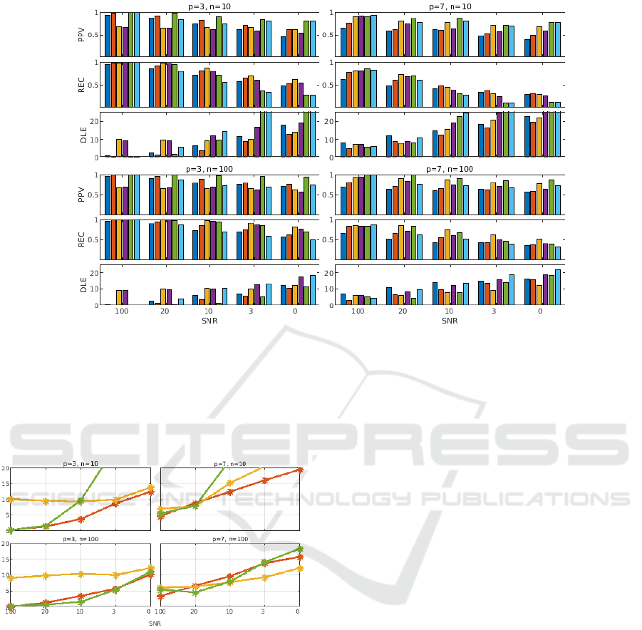
Figure 2: Comparison of localization performance for the six core algorithms: Block-SBR (blue bar), Block-SBR-R1 (red
bar), RAP-MUSIC-o (yellow),TRAP-MUSIC-o (magenta), RAP-MUSIC (green), TRAP-MUSIC (cyan). Algorithms marked
with ‘-o’ indicate versions using an overestimated source space (see main text). The figure is structured in 4 panels, for
different degrees and types of sparsity: up-left, few sources and few number of data points (p = 3, n = 10); up-right, more
sources and few data points (p = 7, n = 10); bottom-left, few sources, more data points (p = 3, n = 100); bottom-right,
more sources and more data points (p = 7, n = 100). For each situation/ panel, we present 3 performance metrics: Positive
Predicted Value (PPV), Recall (REC), and Distance Localization Error (DLE). Block-SBR-R1 consistently demonstrates
superior performance, particularly in sparse configurations (see text for a more detailed discussion).
Figure 3: DLE criterion for the 3 best algorithms: Block-
SBR-R1 (red curve), RAP-MUSIC-o (yellow) and RAP-
MUSIC (green). The four panels illustrate different degrees
of sparsity, in terms of number of active sources p and data
points n. Values of DLE above 20 mm are discarded, the
error is out of reasonably acceptable bounds.
events or narrow band sources localization), as well
as for other sparse signal reconstruction problems.
Clearly, the proposed methods need to be vali-
dated on real data. Work is in progress on this topic,
with the inherent limitations when doing source lo-
calization in brain problems: absence of ground truth
(although, in some clinical setups, conjectures can be
made using other imaging techniques such as fMRI),
artifact and noise contamination, particularities of the
lead-field matrices when considering surface or in-
tracerebral EEG electrodes, etc. Some preliminary
real data results can be found in Hernandez-Castañon
(2023).
Despite its promising performance, the con-
strained block-stepwise regression algorithm is not
without limitations. One consideration is the com-
putational cost associated with iterative optimization
and the computational demands of applying the rank
constraint on regression matrices, which could im-
pose challenges when scaling the method to very large
datasets of high-resolution brain models. Future work
should include developing strategies to enhance com-
putational efficiency and assess the algorithm’s scala-
bility in such scenarios. The actual Matlab implemen-
tations are available upon request, but curated scripts
and functions will be available to download together
with detailed comparisons with other state of the art
algorithms.
5 CONCLUSION
We have introduced in this paper a constrained block
version of a stepwise regression algorithm aiming
to tackle the brain sources localization problem in
Greedy Brain Source Localization with Rank Constraints
825

sparse situations (few number of sources and few data
points). We give convergence and sub-optimality re-
sults. The proposed algorithm is evaluated in compar-
ison with classical state of the art methods in realistic
simulated situations. More results, including in fre-
quency domain on narrow band data, as well as on
real (S)EEG signals will be presented elsewhere.
REFERENCES
Aharon, M., Elad, M., and Bruckstein, A. (2006). K-SVD:
An algorithm for designing overcomplete dictionaries
for sparse representation. IEEE Transactions on Sig-
nal Processing, 54(11):4311–4322.
Baillet, S., Mosher, J., and Leahy, R. (2001). Electromag-
netic brain mapping. IEEE Signal Processing Maga-
zine, 18(6):14–30.
Becker, H., Albera, L., Comon, P., Gribonval, R., Wendling,
F., and Merlet, I. (2014). A performance study of var-
ious brain source imaging approaches. In IEEE Inter-
national Conference on Acoustics, Speech and Signal
Processing (ICASSP), pages 5869–5873.
Dale, A. M. and Sereno, M. I. (1993). Improved Local-
izadon of Cortical Activity by Combining EEG and
MEG with MRI Cortical Surface Reconstruction: A
Linear Approach. Journal of Cognitive Neuroscience,
5(2):162–176.
Fonov, V., Evans, A. C., Botteron, K., Almli, C. R., McK-
instry, R. C., and Collins, D. L. (2011). Unbiased
average age-appropriate atlases for pediatric studies.
NeuroImage, 54(1):313 – 327.
Gramfort, A., Strohmeier, D., Haueisen, J., Hämäläinen,
M., and Kowalski, M. (2013). Time-frequency mixed-
norm estimates: Sparse M/EEG imaging with non-
stationary source activations. NeuroImage, 70:410–
422.
Hämäläinen, M. S. and Ilmoniemi, R. J. (1994). Interpret-
ing magnetic fields of the brain: minimum norm esti-
mates. Medical & Biological Engineering & Comput-
ing, 32(1):35–42.
He, B., Sohrabpour, A., Brown, E., and Liu, Z. (2018).
Electrophysiological source imaging: A noninvasive
window to brain dynamics. Annual Review of Biomed-
ical Engineering, 20(1):171–196.
He, B., Yang, L., Wilke, C., and Yuan, H. (2011). Electro-
physiological imaging of brain activity and connectiv-
ity - challenges and opportunities. IEEE Transactions
on Biomedical Engineering, 58(7):1918–1931.
Hernandez-Castañon, V. (2023). Localization of brain os-
cillatory sources from (S)EEG recordings. PhD thesis,
Université de Lorraine.
Korats, G., Cam, S. L., Ranta, R., and Louis-Dorr, V.
(2016). A space-time-frequency dictionary for sparse
cortical source localization. IEEE Transactions on
Biomedical Engineering, 63(9):1966–1973.
Le Cam, S., Ranta, R., Caune, V., Korats, G., Koessler, L.,
Maillard, L., and Louis-Dorr, V. (2017). SEEG dipole
source localization based on an empirical bayesian ap-
proach taking into account forward model uncertain-
ties. NeuroImage, 153(Supplement C):1 – 15.
Logothethis, N., Kayser, C., and Oeltermann, A. (2007). In
vivo measurement of cortical impedance spectrum in
monkeys: Implications for signal propagation. Neu-
ron, 55:809–823.
Mäkelä, N., Stenroos, M., Sarvas, J., and Ilmoniemi, R. J.
(2018). Truncated RAP-MUSIC (TRAP-MUSIC) for
MEG and EEG source localization. NeuroImage,
167:73–83.
Michel, C., Murray, M., Lantz, G., Gonzalez, S., Spinelli,
L., and Grave de Peralta, R. (2004). EEG source imag-
ing. Clinical neurophysiology, 115(10):2195–2222.
Mosher, J. C. and Leahy, R. M. (1999). Source localiza-
tion using recursively applied and projected (RAP)
MUSIC. IEEE Transactions on Signal Processing,
47(2):332–340.
Pascual-Marqui, R. D. (2007). Discrete, 3D dis-
tributed, linear imaging methods of electric neu-
ronal activity. Part 1: exact, zero error localiza-
tion. arXiv:0710.3341 [math-ph], 2007-October-17,
http://arxiv.org/pdf/0710.3341, pages 1–16.
Ranta, R., Le Cam, S., Tyvaert, L., and Louis-Dorr, V.
(2017). Assesing human brain impedance using si-
multaneous surface and intracerebral recordings. Neu-
roscience, 343:411–422.
Soussen, C., Idier, J., Brie, D., and Duan, J. (2011).
From Bernoulli-Gaussian deconvolution to sparse sig-
nal restoration. Signal Processing, IEEE Transactions
on, 59(10):4572–4584.
Soussen, C., Idier, J., Duan, J., and Brie, D. (2015).
Homotopy based algorithms for ℓ
0
-regularized least-
squares. IEEE Transactions on Signal Processing,
63(13):3301–3316.
BIOSIGNALS 2025 - 18th International Conference on Bio-inspired Systems and Signal Processing
826