Quantum Approaches to the 0/1 Multi-Knapsack Problem: QUBO

Formulation, Penalty Parameter Characterization and Analysis

Evren Guney

1 a

, Joachim Ehrenthal

2 b

and Thomas Hanne

2 c

Department of Industrial Engineering, MEF University, Maslak, Istanbul, Turkey

School of Business, University of Applied Sciences and Arts Northwestern Switzerland FHNW, Brugg, Switzerland

Keywords:

Multi-Knapsack Problem, Quadratic Unconstrained Binary Optimization, Gate-Based Quantum Computing,

Quantum Annealing, Quantum Simulation, Quantum Approximate Optimization Algorithm.

Abstract:

The 0/1 Multi-Knapsack Problem (MKP) is a combinatorial optimization problem with applications in lo-

gistics, ﬁnance, and resource management. Advances in quantum computing have enabled the exploration

of problems like the 0/1 MKP through Quadratic Unconstrained Binary Optimization (QUBO) formulations.

This work develops QUBO formulations for the 0/1 MKP, with a focus on optimizing penalty parameters for

encoding constraints. Using simulation experiments across quantum platforms, we evaluate the feasibility of

solving small-scale instances of the 0/1 MKP. The results provide insights into the challenges and opportuni-

ties associated with applying quantum optimization methods for constrained resource allocation problems.

1 INTRODUCTION

The 0/1 Multi-Knapsack Problem (MKP) extends the

classical knapsack problem to involve multiple knap-

sacks, each with its own capacity constraints. In this

problem, a set of items is available, each characterized

by a proﬁt and weight. The objective is to determine

how to assign these items to knapsacks such that the

total proﬁt is maximized while ensuring that the total

weight in each knapsack does not exceed its capacity.

Additionally, each item can be placed in at most one

knapsack.

The 0/1 MKP is a well-known NP-hard problem,

presenting computational challenges as the number

of items and knapsacks increases. Classical opti-

mization methods, such as exact algorithms, heuris-

tics, and meta-heuristics, have been effective for

solving small- to medium-scale instances. How-

ever, larger problem instances, particularly those

with more complex constraints, require alternative

approaches to address scalability and computational

limitations—despite the recent growth in compute

power.

Quantum computing offers an alternative to clas-

sical optimization by using quantum principles such

https://orcid.org/0000-0001-7572-8627

https://orcid.org/0000-0003-2195-1465

https://orcid.org/0000-0002-5636-1660

as superposition and entanglement to explore solution

spaces more efﬁciently. Advances in quantum hard-

ware and algorithms have enabled early investigations

into solving combinatorial optimization problems on

quantum simulators and devices. These devices pre-

dominantly operate on Quadratic Unconstrained Bi-

nary Optimization (QUBO) models, making them

well-suited for initial research into problems such as

0/1 MKP alongside classical optimization approaches

(Lucas (2014); Glover et al. (2022)).

A fundamental distinction between classical and

quantum methods, such as those using QUBO, lies in

their handling of constraints. Classical methods typi-

cally model constraints explicitly, ensuring feasibility

through structured formulations. In contrast, QUBO

models incorporate constraints directly into the ob-

jective function via penalty parameters. The effec-

tiveness of solving the 0/1 MKP on quantum devices

depends on the calibration of these penalty parame-

ters, as they inﬂuence both the feasibility of solutions

and algorithmic performance. These parameters may

need to be adjusted according to the quantum plat-

form or speciﬁc characteristics of the device, intro-

ducing additional complexity (Glover et al. (2019);

Pecyna and R

zycki (2024)).

Today’s dominant platforms are annealing and

gate-based systems. Quantum annealers (e.g., D-

Wave) natively support QUBO formulations and offer

a direct mapping of optimization problems (Pusey-

Guney, E., Ehrenthal, J. and Hanne, T.

Quantum Approaches to the 0/1 Multi-Knapsack Problem: QUBO Formulation, Penalty Parameter Characterization and Analysis.

DOI: 10.5220/0013387700003890

Paper published under CC license (CC BY-NC-ND 4.0)

In Proceedings of the 17th International Conference on Agents and Artiﬁcial Intelligence (ICAART 2025) - Volume 1, pages 815-823

ISBN: 978-989-758-737-5; ISSN: 2184-433X

815

Nazzaro and Date (2020)), while gate-based quan-

tum computers (e.g., IBM, Google, Quantinuum,

IonQ) implement them through parameterized circuits

(Arute et al. (2019)). These platforms differ in how

they handle QUBO constraints and penalty parame-

ters. By examining these differences experimentally,

this work aims to provide practical insights into the

current applicability and limitations of quantum plat-

forms and their role alongside classical optimization

methods.

Characterizing and optimizing penalty parameters

in QUBO formulations is an under-explored area in

quantum optimization. In earlier work, Boros and

Hammer (2002) introduced the sum of coefﬁcients

method for pseudo-Boolean optimization problems

and reﬁned it through posiform transformations of

QUBO formulations (Boros et al. (2006)). In the

context of quantum computing, initial characteriza-

tions of penalty parameters for various QUBO prob-

lems are provided by Lucas (2014) and Glover et al.

(2022). For knapsack problems speciﬁcally, Quin-

tero and Zuluaga (2021) offered a characterization of

penalty parameters, while recent studies by Awasthi

et al. Awasthi et al. (2023) explored quantum com-

puting techniques for the MKP without focusing on

the characterization of the penalty parameters, where

similar penalty coefﬁcients to our work are proposed.

Further, the work by Verma and Lewis (2022)

presents a general method for determining effective

penalty parameter values in QUBO problems. As-

suming minimization problems, the authors devel-

oped a heuristic to derive suitable lower bounds for

penalty parameters. Building on this, Garc

ıa et al.

(2022) introduced a sequential algorithm to reﬁne

penalty parameters and validated their approach on

classical optimization problems. These studies pro-

vide a foundation for our research into penalty param-

eter characterization in quantum optimization.

Lastly, the 0/1 MKP, characterized by discrete

variables and multiple constraints, naturally aligns

with the QUBO formulations. This property, cou-

pled with the non-fractional structure of the prob-

lem, makes it an ideal candidate for exploring the po-

tential of quantum optimization. Beyond its intrin-

sic optimization challenges, the MKP may also serve

as a benchmark for platform-agnostic testing of op-

timization techniques on the competing current and

near-term quantum device architectures (Dam et al.

(2021)).

This work contributes to the foundational under-

standing of applying quantum computing to the MKP

by:

• Developing a QUBO formulation for the 0/1

MKP, addressing practical scenarios and con-

straints to enhance the applicability and accuracy

of these models in quantum settings.

• Providing a detailed analysis of penalty parame-

ters, which are used to encode constraints within

MKP-QUBO models. We expect the proper char-

acterization of these parameters to impact the fea-

sibility of solutions and the efﬁciency of optimiza-

tion algorithms.

• Conducting simulation experiments to evaluate

the proposed formulations on current quantum

platforms. These experiments offer insights into

the practical performance and limitations of the

models across different quantum computing plat-

forms, providing benchmarks against a current

state-of-the-art solver and for future studies.

The remainder of the paper is structured as fol-

lows: Section 2 outlines the mathematical formu-

lation of the 0/1 MKP and the characterization of

penalty parameters essential for constraint encoding.

Section 3 presents the quantum optimization methods

employed in this study. Section 4 describes the exper-

imental setup and discusses the results obtained from

implementing the formulations on available quantum

devices. Finally, Section 5 concludes with a sum-

mary of ﬁndings and potential directions for future

research.

2 MATHEMATICAL MODELS

The 0/1 MKP is among the most extensively studied

variations of the classical knapsack problem, distin-

guished by involving multiple knapsacks rather than

a single one. The objective is to allocate a set of items

across multiple knapsacks, each with its own capacity,

to maximize the total proﬁt while ensuring the weight

assigned to any knapsack does not exceed its capac-

ity. Formally, given a set of items N , where each

item has a proﬁt c

speciﬁc to a particular knapsack

and a weight d

, and a set of knapsacks K , each with

a capacity E

, the problem is to determine the opti-

mal distribution of items across the knapsacks. To

achieve this, binary decision variables x

are intro-

duced, where x

= 1 if item i is assigned to knap-

sack k, and x

= 0 otherwise. Without loss of gen-

erality, all parameters c, d, and E are assumed to be

non-negative integers.

The 0/1 MKP can be mathematically formulated

as follows:

QAIO 2025 - Workshop on Quantum Artiﬁcial Intelligence and Optimization 2025

816

MKP:

max f (x) =

∑

k=1

∑

i=1

(1)

s.t.

∑

i=1

≤ E

, k ∈ K (2)

∑

k=1

≤ 1, i ∈ N (3)

∈ {0, 1}, i ∈ N ,k ∈ K (4)

In this formulation, the objective function (1) is de-

signed to maximize the total proﬁt of the selected

items. The knapsack capacity constraints (2) ensure

that the total weight assigned to each knapsack k does

not exceed its capacity E

. Additionally, a second set

of constraints (3) prevents any item from being placed

in more than one knapsack. Finally, the binary restric-

tions on the decision variables are speciﬁed in (4).

To construct the QUBO formulation of the MKP,

slack variables u ∈ {0,1}

×K

are introduced for the

constraints in (2), while another set of slack variables

v ∈ {0,1}

is introduced for the constraints in (3).

These constraints are then incorporated into the ob-

jective function by scaling them with penalty param-

eters λ

and λ

, respectively, resulting in the penalty

function P(x,u,v).

P(x,u,v) = λ





∑

k=1

∑

i=1

−

−1

∑

t=0

− α





+ λ





∑

i=1

∑

k=1

+ v

− 1





(5)

Here, M

= ⌊log

⌋ and α

= E

+ 1 − 2

, k ∈

K . It is important to note that when the polynomi-

als are expanded, the penalty function P(x, u,v) in-

cludes a constant term Nλ

due to the 1 present in

the second penalty term. However, as the removal of

constant terms does not affect the optimal solution,

we proceed under the assumption that P(x, u,v) con-

tains only variable-dependent terms, with the constant

term omitted. The resulting QUBO formulation for

the MKP is presented below.

MKP-QUBO:

max g(x,u,v) =

∑

k=1

∑

i=1

− P(x,u,v)

∈ {0,1},i ∈ N , k ∈ K ,t ∈ M

(6)

(7)

Theorem 1. For any penalty constant λ

and λ

such

that λ

≥ C

∗

and λ

≥ C

∗

, where C

∗

= max{c

: i ∈

N , k ∈ K } ,(MKP-QUBO) is a valid reformulation of

the 0/1 multi-knapsack problem (MKP).

Proof. Let x

∗

be an optimal solution for (MKP). Let α

denote the set of coefﬁcients for u in its binary expan-

sion form. Since x

∗

is a feasible solution for (MKP),

there exists u

∗

such that d

∗

= α

∗

for each k ∈ K ,

satisfying the constraints in (2). Similarly, there exists

∗

such that the constraints in (3) are satisﬁed, leading

to g(x

∗

) = c

∗

= f (x

∗

Now consider ( ˆx, ˆu, ˆv), an optimal solution

to (MKP-QUBO). By construction, g( ˆx, ˆu, ˆv) ≥

g(x

∗

) = f (x

∗

), as (x

∗

) is also a feasible

solution to (MKP-QUBO).

To complete the proof, we need to demonstrate

that g( ˆx, ˆu, ˆv) ≤ g(x

∗

) = f (x

∗

) by establishing

that ˆx is also a feasible solution to (MKP). We will

do so by contradiction, showing that an infeasible so-

lution x

′

, which is feasible for MKP-QUBO but not

for MKP, cannot yield a higher objective value. In

this sense, our proof strategy differs from the one

in (Quintero and Zuluaga (2021)). Assume x

∗

the optimal solution to (MKP). We construct an in-

feasible solution x

′

for (MKP) and demonstrate that

g(x

′

) ≤ g(x

∗

) = f (x

∗

) always holds.

Select an index pair ( j,m) from the complement

of the support of x

∗

, that is, ( j,m) ∈ supp

(x) =

{(i,k) | x

∗

= 0}. Set x

= 1. By doing so, we are

adding an extra item j to knapsack m, which results

in an infeasible solution for (MKP). Let x

′

denote this

modiﬁed solution.

Next, we construct the corresponding (MKP-

QUBO) objective by isolating x

in the objective

function. We explicitly display the penalty terms as-

sociated with the m-th and j-th constraints, while in-

troducing P

to represent the remaining penalty terms

of P:

Set x

= 1. In this case, we are adding an extra

item j into knapsack m, which should result in an in-

feasible solution for (MKP). Let’s represent the new

(extended) solution as x

′

. Next, one can construct the

following (MKP-QUBO) by simply separating x

from the objective function and also displaying ex-

plicitly the m-th and j-th penalty terms corresponding

to respective constraints and thus introducing P

the rest of the penalty function P:

g(x

′

) =

∑

k=1

∑

i=1

′

− λ

∑

k=1

∑

i=1

′

−

∑

t=0

′

− λ

∑

i=1

∑

k=1

′

+ v

′

− 1

=g(x

∗

) + c

′

− λ

∑

i=1

′

−

∑

t=0

′

− λ

∑

k=1

′

+ v

′

− 1

− P

′

)

Quantum Approaches to the 0/1 Multi-Knapsack Problem: QUBO Formulation, Penalty Parameter Characterization and Analysis

817

Since x

∗

is optimal for (MKP), it follows that

f (x

∗

) = g(x

∗

). Additionally, P

′

) = 0,

as it does not include any terms involving x

and cor-

responds to constraints that are already satisﬁed.

Let us deﬁne F as the sum of the additional

terms in the last equation, excluding g(x

∗

) and

′

). The key question is whether, with the

current choices for λ

and λ

, it always holds that

F ≤ 0. This ensures that g(x

′

) ≤ g(x

∗

thereby preserving the optimality of the solution

∗

) for (MKP-QUBO).

Since x

′

is infeasible for (MKP), it must violate

either the m-th knapsack capacity constraint or the j-

th knapsack choice constraint, or both. Let us ﬁrst

assume that only the m-th capacity constraint is vio-

lated.

In this case,

∑

i=1

′

−

∑

t=0

′

> 0, with

the minimum magnitude of violation occurring when

∑

t=0

′

= E

, which implies u

′

= 1 for t =

0,.. .,M

. Under the assumption that the second con-

straint is not violated, even when x

′

= 1, it must be

the case that

∑

k=1

∗

= 0. To offset the associated

penalty, we set v

∗

= 1.

When x

′

= 1, then

∑

k=1

′

= 1, and the penalty

can once again be offset by setting v

′

= 0. Conse-

quently, the term associated with λ

can be omitted,

and the total change in the objective function is given

by:

F = c

− λ

∑

i=1

′

− E

Given that λ

≥ C

∗

, the following relationship

holds:

∑

i=1

′

− E

≥ λ

≥ C

∗

≥ c

(8)

Let us now consider the case where adding the ex-

tra item does not cause an overﬂow in the m-th knap-

sack capacity constraint but instead results in a viola-

tion of the j-th single-choice constraint. In this sce-

nario, we have



∑

i=1

′

− E



≤ 0. Consequently,

there exists a solution u

′

such that

∑

t=0

′

∑

i=1

′

, which compensates for the penalty term

associated with the ﬁrst constraint.

The violation of the second constraint, in this case,

is exactly 1, as this constraint has not been previously

violated due to x

∗

= 0. Thus, we can express the

change in the objective function as F = c

− λ

. We

conclude that F ≤ 0 through the following relation-

ship:

≥ C

∗

≥ c

, (9)

where C

∗

represents the maximum proﬁt coefﬁcient.

If both constraints are violated, we can combine

the individual results to construct the following rela-

tionship, which ensures that F < 0:

∑

i=1

′

− E

+ λ

≥ λ

+ λ

≥ 2C

∗

> c

(10)

Thus, when F < 0, it follows that g(x

∗

) >

g(x

′

), indicating that an infeasible solution for

(MKP) cannot yield a higher objective value in

(MKP-QUBO). Consequently, this scenario cannot

occur. Therefore, if λ

> C

∗

and λ

> C

∗

, then x

∗

is both optimal and feasible for (MKP-QUBO).

In the boundary case where λ

= C

∗

and λ

= C

∗

the same conclusion holds. It is possible to construct

a feasible solution ( ˆx, ˆu, ˆv) from (x

′

), indicat-

ing that ( ˆx, ˆu, ˆv) is an alternative optimal solution for

(MKP-QUBO). Hence, we have:

g(x

′

) = g( ˆx, ˆu, ˆv) = c

ˆx ≤ c

∗

= f (x

∗

An interesting observation arises in the third sce-

nario, where both constraints are violated. In this

case, the condition requiring each penalty parameter

to be at least C

∗

may be overly restrictive. The coef-

ﬁcient of λ

can be as large as d

∗

= max{d

: i ∈ N}.

Therefore, as long as d

∗

+ λ

≥ C

∗

, both formula-

tions will produce the same optimal solution, which

depends heavily on the problem data.

3 SOLUTION METHODOLOGY

To address the MKP instances generated for this

study, we employ four distinct solution methods:

(i) solving the classical integer linear programming

(ILP) formulation of MKP using a commercial solver,

(ii) solving the QUBO formulation of MKP with a

commercial solver, (iii) utilizing Quantum Anneal-

ing, and (iv) applying the Quantum Approximate Op-

timization Algorithm (QAOA). State-of-the-art com-

mercial solvers are highly effective at solving both

the ILP and QUBO formulations of MKP by leverag-

ing advanced operations research techniques. These

solvers are mature, well-developed, and fall outside

the primary focus of this work.

In the following, we provide a brief overview of

these two quantum techniques and their relevance to

solving MKP instances.

QAIO 2025 - Workshop on Quantum Artiﬁcial Intelligence and Optimization 2025

818

3.1 Quantum Annealing

Quantum annealing exploits the physical properties of

quantum systems to solve optimization problems (Al-

bash and Lidar (2018)). The underlying principle is

rooted in physics: a system will naturally evolve to-

ward its lowest energy state, also known as its ground

state (Das and Chakrabarti (2008)). In quantum an-

nealing, a problem is encoded into an entangled quan-

tum system where each qubit represents a binary vari-

able in the QUBO formulation. The system is conﬁg-

ured such that its minimum energy state corresponds

to the optimal solution of the problem. Upon mea-

surement, the quantum system collapses, with each

qubit assuming a binary value of 0 or 1, providing the

solution (D-Wave (2022)).

In practice, quantum annealing maps each binary

variable of the optimization problem onto a qubit. In-

teractions between these variables are represented as

qubit entanglements, forming a network that encodes

the problem’s constraints and objective. The goal is to

structure the quantum system so that its ground state

aligns with the optimal solution of the QUBO. Penalty

parameters are used to enforce constraints by assign-

ing higher energy to infeasible solutions, modifying

the energy landscape to guide the system toward fea-

sible conﬁgurations. These parameters must be set

to balance enforcing constraints while preserving the

objective function. This ensures that feasible solu-

tions are energetically favorable compared to infeasi-

ble ones. However, due to the architectural limitations

of quantum hardware, such as restricted qubit connec-

tivity, additional qubits may be required to embed the

problem, which increases resource demands.

The annealing process begins by initializing the

qubits in a superposition state, representing all possi-

ble solutions simultaneously. As the system evolves,

it is guided toward conﬁgurations of progressively

lower energy. At the conclusion of the process, the

system is measured, causing the qubits to collapse

into a classical state of either 0 or 1. Each combina-

tion of these states has an associated energy, which re-

ﬂects the value of the QUBO objective function. The

solution with the lowest energy corresponds to the op-

timal conﬁguration.

The energy landscape of a quantum annealer is a

visualization of the energy values across all possible

conﬁgurations. For instance, Figure 1 illustrates the

energy landscape for a hypothetical QUBO instance

with four binary variables, resulting in 2

= 16 pos-

sible solutions. The height of each state in the land-

scape represents its corresponding energy, including

contributions from penalty terms that distinguish fea-

sible and infeasible solutions. States such as 0011 and

Figure 1: Energy landscape illustration for a hypothetical

QUBO instance with 4 binary variables.

1100 are shown with higher energy, indicating subop-

timal solutions.

3.2 Quantum Approximate

Optimization Algorithm (QAOA)

The Quantum Approximate Optimization Algorithm

(QAOA) is a widely studied variational quantum algo-

rithm developed to tackle combinatorial optimization

problems that are challenging for classical methods

(Blekos et al. (2024)). QAOA falls under the cate-

gory of hybrid quantum-classical algorithms and op-

erates on gate-based quantum computers. The algo-

rithm constructs a parameterized quantum circuit us-

ing a sequence of quantum gates that encode the opti-

mization problem. This circuit alternates between two

types of gates, each associated with a speciﬁc Hamil-

tonian: (i) the Cost Hamiltonian, which represents the

objective function (e.g., a QUBO problem), and (ii)

the Mixer Hamiltonian, which facilitates exploration

of the solution space. Together, these gates form a sin-

gle ”layer” of the QAOA circuit, and multiple layers

can be stacked to improve performance (Farhi et al.

(2014)).

QAOA is designed to run on gate-based quan-

tum devices, including those based on superconduct-

ing qubits (such as IBM and Rigetti systems) or

trapped ions (such as IonQ). The algorithm intro-

duces two tunable parameters, γ (associated with the

Cost Hamiltonian) and β (associated with the Mixer

Hamiltonian), which are iteratively reﬁned using a

classical non-linear optimization routine. γ deter-

mines the system’s alignment with the objective func-

tion, inﬂuencing the depth of energy minimization,

while β controls the degree of exploration in the solu-

tion space. Together, these parameters guide the sys-

tem toward an optimal conﬁguration by balancing ex-

ploitation and exploration. This iterative process uses

feedback from quantum measurements to adjust the

circuit parameters, forming a hybrid algorithm that

integrates classical optimization with quantum exe-

Quantum Approaches to the 0/1 Multi-Knapsack Problem: QUBO Formulation, Penalty Parameter Characterization and Analysis

819

Figure 2: Quantum circuit used in QAOA.

cution. While the quantum component (circuit ex-

ecution) is fully gate-based, the overall process in-

corporates a classical optimization loop (Farhi et al.

(2014)).

Figure 2 illustrates the quantum circuit for a small

QUBO instance with four binary variables. The prob-

lem data is directly encoded into the circuit through

speciﬁc rotations determined by the coefﬁcients of the

QUBO terms. The Mixer Hamiltonian is then applied,

completing one iteration of the QAOA process. Fol-

lowing the optimization of the parameters γ and β,

the circuit is sampled, ideally with a large number of

shots, to identify the conﬁguration that minimizes the

system’s energy with the expectation of this conﬁg-

uration to yield the optimal solution of the original

optimization problem. These parameters hence affect

the quantum state’s evolution during the circuit execu-

tion, shaping the energy landscape such that the sys-

tem is steered toward low-energy conﬁgurations cor-

responding to optimal or near-optimal solutions.

QAOA includes several adjustable settings, such

as the number of circuit layers, the method for initial-

izing parameters, and the choice of classical optimiza-

tion technique. The actual circuits used in quantum

hardware are often more complex than the illustrative

example provided here. These variations in settings

and implementation details signiﬁcantly impact the

performance of the algorithm on practical optimiza-

tion problems.

4 EXPERIMENTAL ANALYSIS

This section examines how penalty parameter cali-

bration inﬂuences the performance of quantum opti-

mization methods for the MKP. Experiments are con-

ducted using a simulation-based approach, enabling

controlled testing of parameter adjustments under

practical constraints. By generating diverse problem

instances and varying penalty parameter values, we

analyze their impact on solution feasibility, quality,

and computational efﬁciency across different quan-

tum technologies, with classical optimization results

provided for comparison.

4.1 Testbed

Our testbed comprises randomly generated MKP

instances, with the number of items set to N ∈

{3,4,5, 6} and the number of knapsacks varying as

K ∈ {2,3}. The revenue values c are randomly chosen

as integers in the range [1, 10], while the item weights

d are selected as random integers within [1, 5]. The

capacities of the knapsacks, E, are also generated ran-

domly as integers between 60% and 80% of the to-

tal weight of items assignable to that knapsack. This

range ensures that not all items can be placed simul-

taneously.

For the penalty parameters λ, the default value is

set as λ = C

∗

= max{c

}. To evaluate the impact of

penalty parameter scaling, a multiplier ranging from

0.5 to 1.5 is applied to λ, with increments of 0.02,

generating a total of 50 distinct λ values. This setup

allows us to investigate the potential for smaller λ val-

ues to cause infeasibility, as well as to analyze how

the magnitude of λ affects solution times.

In total, 4 × 2 × 50 = 300 problem instances are

created. Note that these instances are relatively

small compared to the size of MKP instances typi-

cally solvable by classical computers. However, due

to the limited number of qubits available in current

Noisy Intermediate-Scale Quantum (NISQ) quantum

devices, solving larger problem instances efﬁciently

is not feasible with the present state of quantum tech-

nology.

4.2 Experimental Setup and

Implementation Details

To generate the problem instances, we developed a

C# console application using Microsoft Visual Stu-

dio Community 2022. Both the classical MIP for-

mulation and the QUBO formulation of the MKP in-

stances were created using Gurobi callable libraries

and solved using the Gurobi 12.0 Solver (Gurobi Op-

timization, LLC (2024)). For the quantum implemen-

tations, the instances were tested across three primary

quantum technologies: gate-based circuits, trapped-

ion circuits, and quantum annealing.

For the quantum annealing experiments, we uti-

lized D-Wave libraries (D-Wave (2022)). Using D-

Wave’s Python interface, the QUBO formulation of

each instance was transformed into an optimization

problem and solved using the annealer. For gate-

based quantum experiments, we relied on IBM Qiskit

libraries, where the Q matrix representing the co-

QAIO 2025 - Workshop on Quantum Artiﬁcial Intelligence and Optimization 2025

820

efﬁcients of the QUBO instance was used to con-

struct quantum circuits. A standard QAOA subrou-

tine was then executed to ﬁnd the best solution. In the

QAOA implementation, the circuit dept is chosen to

be p = 3 which is the recommended value in many

works (Blekos et al. (2024)). Qiskit implementation

of QAOA uses the COBYLA solver (Powell (1994))

as the default, non-linear, derivative-free solver to op-

timize the circuit parameters. Finally, the trapped-ion

experiments employed IonQ Python libraries. Similar

to the gate-based approach, circuits were generated

from the Q matrix of each instance and solved using

the QAOA algorithm.

Each instance is run 10 times on the quantum plat-

forms, with a sample size (or number of shots) set

to 10,000. For both annealing and gate-based ap-

proaches, increasing the number of shots mitigates er-

rors inherent to quantum mechanics, improving solu-

tion accuracy. In every experiment, we recorded the

best solution, the corresponding objective value, and

the solution time. Since the MIP solver reliably ﬁnds

the optimal solutions for both the classical MIP and

QUBO formulations, these serve as a benchmark. Ad-

ditionally, we assessed whether the QUBO solutions

obtained from the solver and the three quantum-based

methods were feasible and/or optimal.

4.3 Computational Results

We began by comparing the running times of the ﬁve

methods tested in our experiments, as summarized in

Table 1. These times represent averages over 10 ×

50 = 500 runs (10 randomly generated instances with

50 different values of the penalty parameter) for each

combination of N and K.

In Table 1, the ﬁrst column lists the number of

items (N) and knapsacks (K) for the generated prob-

lem instances. The next two columns show the aver-

age solution times obtained using Gurobi for the clas-

sical integer programming (MIP) and QUBO formu-

lations of the MKP. The ﬁnal three columns present

the average solution times for the quantum-based

methods.

As expected, Gurobi achieved the fastest solution

times for the classical integer programming formu-

lation of the MKP, followed closely by the QUBO

version solved with Gurobi. The D-Wave quantum

annealer demonstrated comparable performance to

Gurobi’s quadratic solver, solving nearly all instances

in under one second. It is notable that D-Wave’s av-

erage running time is smaller than Gurobi’s quadratic

solver for the largest instances corresponding to 5/6

item and 3 knapsack scenarios. In contrast, QAOA-

based methods were signiﬁcantly slower, with solu-

tion times increasing as the problem size grew. For

the largest instances both annealing methods fail to

provide solutions either with out of memory or time-

out errors.

For the IonQ simulator, instances with (N,K) =

(4,3), (5,3), and (6, 3) could not be solved due to

memory limitations, highlighting current hardware

constraints for larger problem sizes.

Table 1: Comparison of running times across different

solvers for varying values of N (number of items) and K

(number of knapsacks).

N,K

Int. Pr. Gur. Qu. Annl. QAOA

IP QUBO D-Wave Qiskit IonQ

3,2 0.003 0.06 0.33 23.1 17.9

4,2 0.003 0.14 0.36 30.5 33.8

5,2 0.012 0.22 0.51 184.1 276.8

6,2 0.124 0.42 0.67 641.1 2075.4

3,3 0.005 0.07 0.40 86.9 209.3

4,3 0.007 0.10 0.44 371.6 -

5,3 0.005 1.15 0.54 - -

6,3 0.005 2.56 0.56 - -

Table 2 compares the solution quality of the

quantum-based methods. Since the optimal solutions

for all instances are known, we evaluate the perfor-

mance of the three quantum-based methods by calcu-

lating the percentage of instances where they success-

fully ﬁnd the optimal solution.

D-Wave achieves the optimal solution in almost

all cases for the smaller size instances but may de-

crease up to 54.6% for most complex cases. For

smaller instances, QAOA-based methods also per-

form well, with IonQ generally outperforming Qiskit.

However, as the instance size increases, the solution

quality of the QAOA-based methods declines signiﬁ-

cantly.

Table 2: Per-cent of Optimal Solutions found by the

quantum-based method.

N,K

Qu. Annl. QAOA

D-Wave Qiskit IonQ

3,2 100.0% 85.3% 92.7%

4,2 99.7% 86.0% 95.9%

5,2 99.8% 71.9% 85.8%

6,2 99.4% 54.8% 66.8%

3,3 99.2% 63.8% 69.0 %

4,3 99.5% 42.2% -

5,3 68.6% - -

6,3 54.6% - -

4.4 Effect of Penalty Parameter

Magnitude on Feasibility

In the proof of Theorem-1, we noted that requiring the

penalty parameter λ to be at least λ = C

∗

= max{c

}

Quantum Approaches to the 0/1 Multi-Knapsack Problem: QUBO Formulation, Penalty Parameter Characterization and Analysis

821

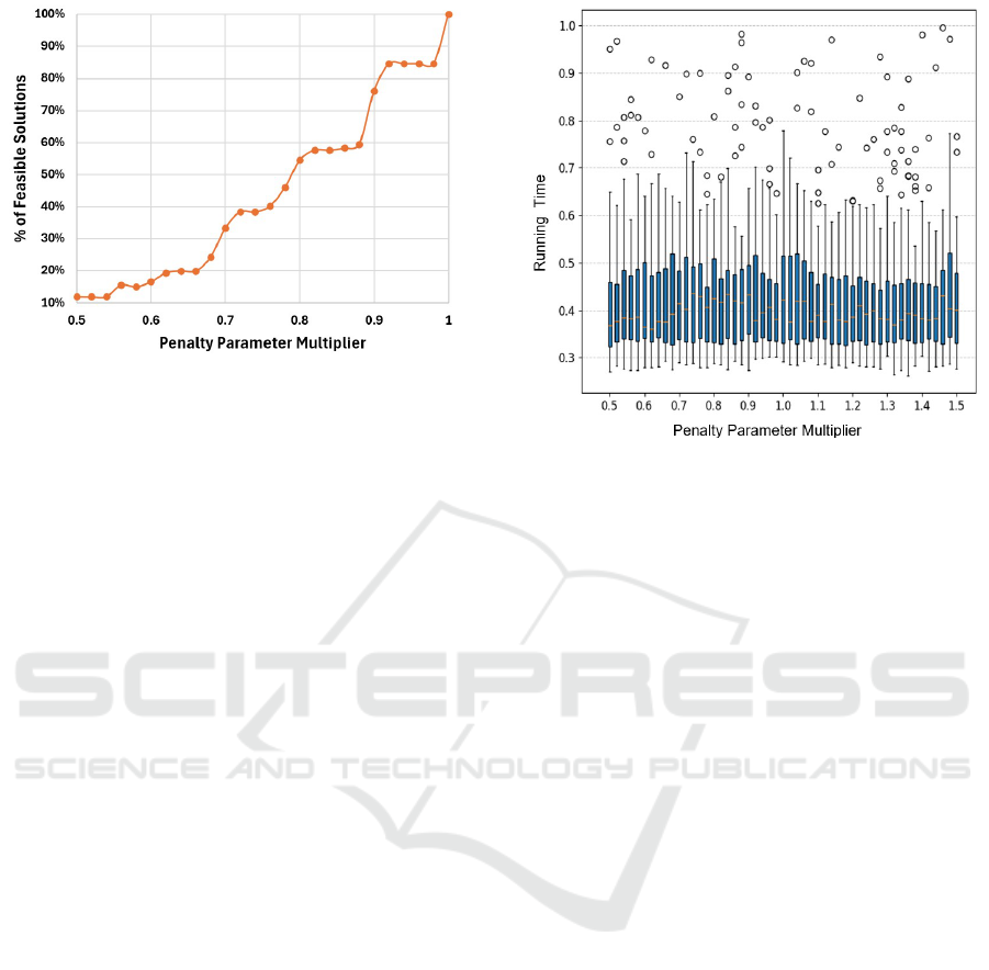
Figure 3: Effect of penalty parameter magnitude on solution

feasibility.

may be overly restrictive for certain instances. To in-

vestigate this, we calibrated the value of λ using a

multiplier ranging from 0.5 to 1.5. Figure 3 illustrates

the average percentage of instances that resulted in

feasible solutions under these varying penalty param-

eter settings.

Each data point in the ﬁgure represents the aver-

age results over 10 × 8 = 80 instances (10 random

instances across 8 different combinations of N and

K). When the penalty parameter coefﬁcient is set to

1.00, λ equals C

∗

, and all QUBO instances produce

the same optimal solutions as the original integer pro-

gramming formulation of the MKP.

However, as the penalty parameter is reduced be-

low this theoretical minimum, a gradual decline in

feasibility is observed, with fewer QUBO solutions

satisfying the constraints of the original MKP. Fu-

ture research could focus on deriving tighter bounds

for penalty parameters tailored to speciﬁc MKP in-

stances, potentially reducing the need for conservative

parameter settings.

4.5 Effect of Penalty Parameter

Magnitude on Solution Duration

Finally, we evaluate how the magnitude of the penalty

parameter affects the running time of the solution

methods. This analysis is based on normalized run-

ning times for 80 instances across 4 QUBO-based

methods. The results, summarized in the box-whisker

plot in Figure 4, indicate that the magnitude of the

penalty parameter has minimal impact on solution

times. A consistent pattern is observed across all indi-

vidual quantum methods (e.g., annealing and QAOA);

hence, more granular plots for speciﬁc methods are

omitted.

Figure 4: Effect of penalty parameter magnitude on running

time.

Note that these results were obtained using classi-

cal quantum system simulators, which may not fully

capture the computational dynamics of actual quan-

tum hardware. Replicating these experiments on real

quantum devices would provide more accurate in-

sights and validate the observations made here.

5 CONCLUSIONS

This study investigates the application of QUBO for-

mulations to the 0/1 Multi-Knapsack Problem (MKP)

using classical and quantum techniques.

Speciﬁcally, we characterize and analyze the

penalty parameters, demonstrating that overly con-

servative settings can impact feasibility without sig-

niﬁcantly affecting solution times. Our results high-

light the strengths and limitations of quantum anneal-

ing and QAOA in solving MKP instances on simu-

lators, with annealing showing potential for handling

larger problem sizes, albeit with suboptimal solutions.

Speciﬁcally for our investigation, a state-of-the-art

classical solver remains superior.

Further, our research suggests exploring better

ways to conﬁgure penalty parameters for annealing,

as well as simplifying quadratic representations to

reduce computational overhead across all platforms,

both quantum and classical. Lastly, testing across a

wider range of simulators and on real quantum de-

vices may further guide scholarly efforts in adopting

quantum techniques for common operations research

problems.

QAIO 2025 - Workshop on Quantum Artiﬁcial Intelligence and Optimization 2025

822

REFERENCES

Albash, T. and Lidar, D. A. (2018). Demonstration of a scal-

ing advantage for a quantum annealer over simulated

annealing. Physical Review X, 8(3):031016.

Arute, F. et al. (2019). Quantum supremacy using a

programmable superconducting processor. Nature,

574(7779):505–510.

Awasthi, A., B

ar, F., Doetsch, J., Ehm, H., Erdmann,

M., Hess, M., Klepsch, J., Limacher, P. A., Luckow,

A., Niedermeier, C., Palackal, L., Pfeiffer, R., Ross,

P., Saﬁ, H., Sch

onmeier-Kromer, J., von Sicard, O.,

Wenger, Y., Wintersperger, K., and Yarkoni, S. (2023).

Quantum computing techniques for multi-knapsack

problems. In Arai, K., editor, Intelligent Computing,

pages 264–284. Springer Nature Switzerland.

Blekos, K., Brand, D., Ceschini, A., Chou, C.-H., Li, R.-

H., Pandya, K., and Summer, A. (2024). A review on

quantum approximate optimization algorithm and its

variants. Physics Reports, 1068:1–66. A review on

Quantum Approximate Optimization Algorithm and

its variants.

Boros, E. and Hammer, P. L. (2002). Pseudo-boolean op-

timization. Discrete Applied Mathematics, 123(1–

3):155–225.

Boros, E., Hammer, P. L., and Tavares, G. (2006). Prepro-

cessing of unconstrained quadratic binary optimiza-

tion. Technical Report RRR 10-2006, Rutgers Univer-

sity, New Jersey, USA. RUTCOR Research Report.

D-Wave (2022). What is quantum annealing? Accessed:

2024-11-11.

Dam, W. v., Eldefrawy, K., Genise, N., and Parham, N.

(2021). Quantum optimization heuristics with an ap-

plication to knapsack problems. In 2021 IEEE Inter-

national Conference on Quantum Computing and En-

gineering (QCE), pages 160–170. IEEE.

Das, A. and Chakrabarti, B. K. (2008). Colloquium: Quan-

tum annealing and analog quantum computation. Rev.

Mod. Phys., 80:1061–1081.

Farhi, E., Goldstone, J., and Gutmann, S. (2014). A quan-

tum approximate optimization algorithm.

Garc

ıa, M. D., Ayodele, M., and Moraglio, A. (2022). Ex-

act and sequential penalty weights in quadratic uncon-

strained binary optimisation with a digital annealer. In

Proceedings of the Genetic and Evolutionary Com-

putation Conference Companion, GECCO ’22, page

184–187, New York, NY, USA. Association for Com-

puting Machinery.

Glover, F., Kochenberger, G., and Du, Y. (2019). A tu-

torial on formulating and using qubo models. arXiv

preprint, arXiv:1811.11538.

Glover, F., Kochenberger, G., Hennig, R., Lewis, M., L

u, Z.,

Wang, H., and Wang, Y. (2022). Quantum bridge ana-

lytics i: a tutorial on formulating and using qubo mod-

els. Annals of Operations Research, 314:141–183.

Gurobi Optimization, LLC (2024). Gurobi Optimizer Ref-

erence Manual.

Lucas, A. (2014). Ising formulations of many np problems.

Frontiers in Physics, 2.

Pecyna, T. and R

zycki, R. (2024). Improving quantum

optimization algorithms by constraint relaxation. Ap-

plied Sciences, 14(18):8099.

Powell, M. J. D. (1994). A direct search optimization

method that models the objective and constraint func-

tions by linear interpolation. Advances in Optimiza-

tion and Numerical Analysis, pages 51–67.

Pusey-Nazzaro, L. and Date, P. (2020). Adiabatic quantum

optimization fails to solve the knapsack problem. Ac-

cessed: 2024-12-04.

Quintero, R. A. and Zuluaga, L. F. (2021). Characterizing

and benchmarking qubo reformulations of the knap-

sack problem. Technical report, Department of In-

dustrial and Systems Engineering, Lehigh University.

Technical Report.

Verma, A. and Lewis, M. (2022). Penalty and partitioning

techniques to improve performance of qubo solvers.

Discrete Optimization, 44:100594. Quadratic Combi-

natorial Optimization Problems.

Quantum Approaches to the 0/1 Multi-Knapsack Problem: QUBO Formulation, Penalty Parameter Characterization and Analysis

823