Investigation of MAPF Problem Considering Fairness and Worst Case
Toshihiro Matsui
a
Nagoya Institute of Technology, Gokiso-cho Showa-ku Nagoya Aichi 466-8555, Japan
Keywords:
Multiagent Pathfinding Problem, Leximin/Leximax, Fairness, Worst Case.
Abstract:
We investigate multiagent pathfinding problems that improve fairness and the worst case among multiple ob-
jective values for individual agents or facilities. Multiagent pathfinding (MAPF) problems have been widely
studied as a fundamental class of problem in multiagent systems. A common objective to be optimized in
MAPF problem settings is the total cost value of the moves and actions for all agents. Another optimization
criterion is the makespan, which is equivalent to the maximum cost value for all agents in a single instance
of MAPF problems. As one direction of extended MAPF problems, multiple-objective problems have been
studied. In general, multiple objectives represent different types of characteristics to be simultaneously op-
timized for a solution that is a set of agents’ paths in the case of MAPF problems, and Pareto optimality is
regarded as a common criterion. Here, we focus on an optimization criterion related to fairness and the worst
case among the agents themselves or the facilities affected by the agents’ plans, and this is also a subset of
the makespan criterion. This involves several situations where the utilities/costs, including robots’ lifetimes
and related humans’ workloads, should be balanced among individual robots or facilities without employing
external payments. The applicability of these types of criteria has been investigated in several optimization
problems, including distributed constraint optimization problems, multi-objective reinforcement learning, and
single-agent pathfinding problems. In this study, we address the case of MAPF problems and experimentally
analyze the proposed approach to reveal its effect, as well as related issues, in this class of problems.
1 INTRODUCTION
We investigate multiagent pathfinding problems that
improve fairness and the worst case among multi-
ple objective values for individual agents or facilities.
Multiagent pathfinding (MAPF) problems have been
widely studied as a fundamental class of problem in
multiagent systems. This problem is the basis for var-
ious systems using agents that simultaneously move
through an environment, such as robot navigation, au-
tonomous taxiing of airplanes, and video games (Ma
et al., 2017).
Various types of optimal and quasi-optimal solu-
tion methods, including the CA* algorithm (Silver,
2005), Conflict Based Search (CBS) (Sharon et al.,
2015), push-and-rotate (De Wilde et al., 2014; Luna
and Bekris, 2011), PIBT (Okumura et al., 2022) and
LaCAM (Okumura, 2023) have been studied. Other
studies have used the solvers of general optimiza-
tion problems or translated the MAPF problem into
a standard optimization problem. Moreover, different
extended classes of problems and dedicated solution
a
https://orcid.org/0000-0001-8557-8167
methods have also been proposed (Miyashita et al.,
2023; Yakovlev and Andreychuk, 2017; Andreychuk
et al., 2022; Andreychuk et al., 2021).
A common target for optimization in MAPF prob-
lem settings is the total cost value of moves and ac-
tions for all agents. Another optimization criterion is
the makespan, which is equivalent to the maximum
cost value for all agents in a single instance of MAPF
problems. As one direction of extended MAPF prob-
lems, multiple-objective problems have been stud-
ied (Weise et al., 2020; Wang et al., 2024). In gen-
eral, multiple objectives represent different types of
characteristics to be simultaneously optimized for a
solution that is a set of agents’ paths in the case of
MAPF problems, and Pareto optimality is regarded
as a common criterion. Here, we focus on an op-
timization criterion related to fairness and the worst
case among the agents themselves or the facilities af-
fected by the agents’ plans, and this is also a sub-
set of the makespan criterion. This involves several
situations where the utilities/costs, including robots’
lifetimes and related humans workloads, should be
balanced among individual robots or facilities with-
224
Matsui, T.
Investigation of MAPF Problem Considering Fairness and Worst Case.
DOI: 10.5220/0013389600003890
Paper published under CC license (CC BY-NC-ND 4.0)
In Proceedings of the 17th International Conference on Agents and Artificial Intelligence (ICAART 2025) - Volume 1, pages 224-234
ISBN: 978-989-758-737-5; ISSN: 2184-433X
Proceedings Copyright © 2025 by SCITEPRESS – Science and Technology Publications, Lda.

out employing external payments. The applicability
of these types of criteria has been investigated in sev-
eral optimization problems, including distributed con-
straint optimization problems (Matsui et al., 2018a;
Matsui et al., 2018c), multi-objective reinforcement
learning (Matsui, 2019), and single-agent pathfinding
problems (Matsui et al., 2018b). In this study, we ad-
dress the case of MAPF problems and experimentally
analyze the proposed approach to reveal its effect, as
well as related issues, in this class of problems.
The rest of this paper is organized as follows. In
the next section, we present the background of our
study, including multiagent pathfinding problems, so-
lution methods, the leximax criterion, and application
of this criterion to pathfinding problems. The details
of our proposed approach are then presented in Sec-
tion 3. We apply the above criterion to the cases of
both agents and facilities on maps We then exper-
imentally investigate these approaches in Section 4
and conclude our paper in Section 5.
2 BACKGROUND
2.1 MAPF Problem
The multiagent pathfinding (MAPF) problem is an
optimization problem to find the set of shortest paths
(sequences of agents’ actions) of multiple agents
where there are no collisions among the paths. A
MAPF problem is generally defined by an undirected
graph G = ⟨V, E⟩ consisting of sets V and E of edges
and vertices representing a two-dimensional map, a
set of agents A, and a set of pairs of start and goal
vertices (v
s
i
, v
g
i
) of individual agents a
i
∈ A, where
v
s
i
, v
g
i
∈ V . Each agent a
i
must move from v
s
i
to v
g
i
without colliding with other agents’ paths, including
stay/wait actions, and the paths should be minimized
with optimization criteria. In a standard setting, all
move/stay actions of agents take the same cost value,
and the sum of costs or the makespan among agents’
paths should be minimized. As a commonly used
assumption, we ignore the existence of agents who
reached their goals. There are two cases of colli-
sion paths; 1) two agents are located at the same ver-
tex at the same time (a vertex collision) and 2) two
agents move on the same edge at the same time from
both ends of the edge (a swapping collision). A typ-
ical basic problem employs a graph based on a four-
connected grid map with obstacles, and it considers
discrete time steps.
While there are different types of solution meth-
ods, we employ our customized version of the Con-
flict Based Search (CBS) algorithm (Sharon et al.,
2015) as a standard base method for the new class of
MAPF problems tackled in this study.
2.2 CBS
The Conflict Based Search (CBS) algorithm (Sharon
et al., 2015) is a fundamental complete solution
method for solving MAPF problems. Although this
type of algorithm faces the issue of limited scalabil-
ity, a simple version is often employed as a base solver
for an extended problem in the first steps of study.
This solution method consists of two layers of
search. In the high-level layer, agents’ collisions
are managed as constraints using a best-first tree-
search algorithm. We employ a version of binary-
tree search. This tree is called a constraint tree (CT),
where its node (CT node) represents a set of paths
for all agents that are individually computed for each
agents. Therefore, a CT node can be evaluated with an
optimization criterion while disregarding collisions of
the agents’ paths. A CT node also has a set of con-
straints (a
i
, v, t). Here, a constraint inhibits agent a
i
from locating at vertex v at time step t. The root CT
node has no constraint, and there can generally be a
degree of conflict among several paths of agents. In
every step in CT search, a single node is selected in
a best-first manner, and the first conflict in the paths,
if one exists, is selected for a pair of agents. For a
vertex conflict (a
i
, a
j
, v, t), two child CT nodes who
individually have one of two new constraints (a
i
, v, t)
and (a
j
, v, t) are expanded. For a swap conflict, two
child CT nodes with the same form of constraint are
generated by considering the agents’ moves. The path
of a
i
or a
j
in a child CT node is then updated under
its new constraint. If there is no conflict among paths
in a selected CT node, that becomes the solution.
In the low-level layer, a pathfinding algorithm on a
time-space graph, such as the A* algorithm (Hart and
Raphael, 1968; Hart and Raphael, 1972; Russell and
Norvig, 2003), is used to find a single agent’s path for
a CT node under its newly imposed constraints. Here,
an agent selects either a move or stay action at each
time step, and each action generally takes one time
step.
Although there are several optimal and quasi-
optimal extended variations (Ma et al., 2019; Barer
et al., 2014) to mitigate the relatively high computa-
tional cost of the optimal search method, we employ a
simple version of CBS under a limited range of prob-
lems for our first study.
Investigation of MAPF Problem Considering Fairness and Worst Case
225

2.3 Multi-Objective Optimization and
Leximin/Leximax
In this study, we focus on a specific case of multiple
objectives involving fairness among agents or among
facilities that are affected by the agents’ paths.
General multi-objective optimization problems
have multiple objective functions that need to be si-
multaneously optimized. A fundamental minimiza-
tion problem is defined as ⟨X, D, F⟩, where X , D, and
F are a set of variables, a set of domains of vari-
ables, and a set of objective functions, respectively.
Variable x
i
∈ X takes a value in finite and discrete
set D
i
∈ D. For the set of variables X
j
⊆ X, the
jth single objective function f
j
(X
j
) ∈ F is defined
as f
j
(x
j,1
, ··· , x
j,k
) : D
j,1
× ··· × D
j,k
→ N, where
x
j,1
, ··· , x
j,k
∈ X
j
. An objective vector v, defined as
[v
1
, ··· , v
k
], represents multiple objective values of the
objective functions, where v
j
= f
j
(A
↓X
j
) for assign-
ment A to the variables in X
j
.
The ideal goal of the problem is to simultaneously
minimize the cost values of all objective functions.
Since this cannot generally be fully achieved due to
trade-offs between the objectives, Pareto optimality
has been considered as a way to filter locally opti-
mal solutions. Moreover, several social welfare crite-
ria and scalarization functions have been employed to
select a solution from a typically enormous number
of Pareto optimal solutions (Sen, 1997; Marler and
Arora, 2004).
Although the minimization on total cost
∑
k
j=1
f
j
(X
j
) is Pareto optimal, it only considers
the global cost value. The minimization on the
maximum cost max
k
j=1
f
j
(X
j
) improves the worst
case (min-max). However, it does not ensure the
Pareto optimality due to its insufficient filtering of
solutions. The ties of maximal cost values are often
broken by summation.
Another criterion based on the maximum cost
value lexicographically compares the cost values in
two objective vectors by repeatedly comparing them
from the worst (maximum) values to the best (mini-
mum) values. This is a variant of leximin (Bouveret
and Lema
ˆ
ıtre, 2009; Greco and Scarcello, 2013; Mat-
sui et al., 2018a; Matsui et al., 2018c) for maximiza-
tion problems, and thus we denote it as leximax.
For minimization problems, we employ vectors of
sorted objective values, which have an inverted order
from that for the leximin case, as well as a comparison
operator (Matsui et al., 2018b).
Definition 1 (Descending sorted objective vector).
The values of a descending sorted objective vector are
sorted in descending order.
Definition 2 (Leximax). Let v = [v
1
, ··· , v
K
] and
v
′
= [v
′
1
, ··· , v
′
K
] denote descending objective vectors
whose lengths are K. The order relation, denoted
as ≺
leximax
, is defined as v ≺
leximax
v
′
if and only if
∃t, ∀t
′
< t, v
t
′
= v
′
t
′
∧ v
t
< v
′
t
.
The minimization on leximax improves the worst
case as a variant of min-max and it also relatively im-
proves the fairness among the objective cost values.
A benefit of this criterion among fairness criteria is
its decomposability. The addition of two descending
sorted objective vectors provides concatenation and
resorting operations.
Definition 3 (Addition of descending sorted objective
vectors). Let v and v
′
denote vectors [v
1
, ··· , v
K
] and
[v
′
1
, ··· , v
′
K
′
], respectively. The addition of two vectors,
v ⊕ v
′
, is represented as v
′′
= [v
′′
1
, ··· v
′′
K+K
′
], where v
′′
consists of all values in v and v
′
. In addition, the
values in v
′′
are sorted in descending order.
The addition of vectors ensures a kind of mono-
tonicity that is necessary in optimization methods
such as tree search and dynamic programming (Mat-
sui et al., 2018a; Matsui et al., 2018b).
Proposition 1 (Invariance of leximax upon addition).
Let v and v
′
denote sorted objective vectors of the
same length. In addition, v
′′
denotes another sorted
objective vector. If v ≺
leximax
v
′
, then v ⊕ v
′′
≺
leximax
v
′
⊕ v
′′
.
When relatively fewer types of discrete objec-
tive values are employed, the descending sorted ob-
jective vector can be represented as a vector of the
sorted pairs of an objective value and the count of
the value (Matsui et al., 2018a; Matsui et al., 2018b).
This run-length encoding is also considered a sorted
histogram, and the redundant length of the original
descending sorted vector is reduced. In addition, the
comparison and addition operators on the encoded
vectors are available.
The applicability of these types of criteria has
been investigated in several optimization prob-
lems, including distributed constraint optimization
problems (Matsui et al., 2018a; Matsui et al.,
2018c), multi-objective reinforcement learning (Mat-
sui, 2019), and single-agent pathfinding prob-
lems (Matsui et al., 2018b).
2.4 Pathfinding by Fairness and Worst
Case Among Individual Edge Costs
In a previous study (Matsui et al., 2018b), the applica-
bility of the leximax criterion was further investigated
for shortest pathfinding problems. Here, each edge
in a graph in a traditional shortest pathfinding prob-
lem has a discrete move cost value within a relatively
ICAART 2025 - 17th International Conference on Agents and Artificial Intelligence
226

1 2 3
4 5 6
7 8 9
1 1
1 1
1 1
1
211
22
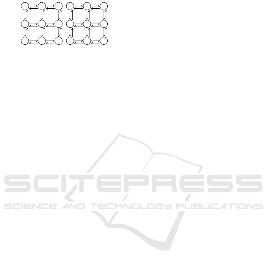
Figure 1: Lattice graph (Matsui et al., 2018b).
limited range such as {1, ..., 5} or {1, ..., 10}, repre-
senting certain cost levels. Then the cost values of
paths are aggregated and compared in the manner of a
leximax criterion using an extended set of descending
sorted objective vectors of arbitrary length.
In Figure 1, one of the optimal paths from start
vertex 1 to goal vertex 9, under the minimization of
conventional total cost values, is (1, 2, 3, 6, 9), and its
cost is 5. In the case of the minimization of the maxi-
mal cost values, one optimal path is (1, 2,3, 6, 5, 8, 9),
where its cost is 6, and the latter path contains no
edges with a cost value of 2. The goal of the problem
is not only to reduce the number of edges with max-
imum cost values but also, if possible, to reduce the
total cost value while improving the fairness among
edges. This problem setting relates to cases where a
route should avoid highly affected residents or extra
loads at bottleneck facilities by compromising tradi-
tional optimality.
To employ best-first search and dynamic program-
ming methods, including the Dijkstra’s algorithm and
the A* algorithm (Hart and Raphael, 1968; Hart and
Raphael, 1972; Russell and Norvig, 2003), the op-
erations of leximax are extended for subproblems of
different lengths of vectors, which represent different
lengths of paths. By extending the leximax to objec-
tive vectors of different lengths, the variable-length
leximax, vleximax, is employed.
Definition 4 (Vleximax). Let v = [v
1
, ··· , v
K
] and
v
′
= [v
′
1
, ··· , v
′
K
′
] denote descending sorted objective
vectors whose lengths are K and K
′
, respectively. For
K = K
′
, ≺
vleximax
is the same as ≺
leximax
. In other
cases, zero values are appended to one of the vectors
so that the both vectors have the same number of val-
ues. Then the vectors are compared based on ≺
leximax
.
This comparison considers two descending sorted
objective vectors that are modified from the original
ones so that these vectors have the same sufficient
length by padding blanks with zero cost values. The
comparison of leximax is based on tie-breaks on ob-
jective values from the beginning of both vectors, and
the redundant last parts of zeros can be ignored.
In the A* search algorithm, vertices are evaluated
with descending sorted objective vectors, and the vec-
tors are appropriately aggregated and compared. In
addition, the heuristic function for the A* algorithm
can be generalized as a lower bound vector that does
not exceed the optimal cost value, while the gap be-
tween an intuitively admissible heuristic distance and
the true one is relatively large.
Moreover, a previous study also addressed the
case of Learning Real-Time A* algorithm (Barto
et al., 1995), which is an on-line search method re-
lated to reinforcement learning. Although the A* al-
gorithm with vleximax performs correctly for tradi-
tional two dimensional maps, the on-line search case
suffers from a property of the criterion. When the
length of descending sorted objective vectors is not
limited, the length of a lower bound vector can glow
infinitely by adding lower bound objective values.
This phenomenon resembles the case of negative cy-
cles in pathfinding problems. As the result, the lower
bound cost vector of a path never reaches a corre-
sponding upper bound cost vector, while the upper
bound can well decrease to the optimal one. Several
approaches can mitigate this issue.
3 APPLICATION OF LEXIMAX
CRITERION TO SOLUTION
METHOD
We extend the MAPF problem by applying a lexi-
max criterion. We address both cases of the leximax
among agents and the vleximax among vertices in all
agents’ paths.
3.1 Extended Problem with Vertex
Costs and Additional Criteria
We employ a MAPF problem where each vertex v in
the graph of a map has a cost c(v) that takes its value
from a relatively limited range of discrete values such
as {1, ..., 5} or {1, ..., 10}. The lower and upper limit
cost values are denoted by c
⊥
and c
⊤
, and we define
that c
⊥
= 0. In the two examples above, c
⊤
must be
greater than 5 and 10. We also define a move/stay cost
c(v
′
, v) = c(v) from vertex v
′
to v for all v
′
adjacent to
v, including the wait action on a time-space graph.
Namely, the graphs are extended to directed graphs.
The traditional MAPF is the case of c(v) = 1.
We employ the CBS algorithm as the basis of a
solution method and apply leximax based operations.
The aggregation and optimization criteria of cost val-
ues in a MAPF problem can be separated into those
among agents’ paths and others among components
in each path. We denote the combination of these two
classes of criteria using the form of (among agent)-
Investigation of MAPF Problem Considering Fairness and Worst Case
227

based on cost of vertices
1 2 3
4 5 6
7 8 9
1
2
2
1
2
(a) cost of vertices
1 2 3
4 5 6
7 8 9
1 2
22
1
1 1
1
(b) cost of edges
1 2 3
4 5 6
7 8 9
1
2
2
1
2
(a) cost of vertices
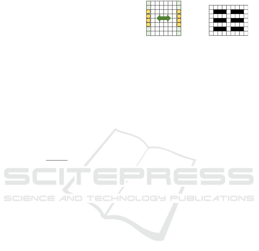
Figure 2: Lattice graph with walls.
(among path element). For a fundamental MAPF
problem, the traditional sum-of-costs is denoted by
sum-sum, while the makespan is identical to max-
sum. We address other cases below.
3.2 Leximax Among Agents
A relatively intuitive extension of leximax-sum ap-
plies the leximax criterion to the cost values among
conventional agents’ paths. The high-level search of
the CBS algorithm is modified to employ the descend-
ing sorted objective vector, aggregation operator, and
comparison operator of leximax for the aggregation
of agents’ paths, while each agent’s pathfinding in the
lower-level is based on the conventional A* algorithm
with the summation of cost values on a time-space
graph.
An objective value in a sorted vector is a cost value
of an individual agent’s path, and the first objective
value is identical to the case of minimizing makespan
(max-sum). The ties of solutions with the makespan
criterion are broken by employing the leximax com-
parison operator. In the minimization of cost vectors
among agents, we simply employ the upper limit cost
value c
⊤
= ∞ as a default value for cost vectors, and
the default upper limit vector contains |A| cost values
of c
⊤
.
Although this case of optimization is a natural ex-
tension of the case of minimizing makespan, it might
cause combinatorial explosion in dense settings of
agents at an earlier stage than the case of makespan.
The leximax criterion could have a bias to expand
a specific CT node with its detailed tie-break in the
high-level search, and it is not possible to ensure that
such CT nodes provide promising results.
3.3 Vleximax Among Vertices
The pathfinding part of each agent in the low-level
search of the CBS algorithm can employ the vlex-
imax criterion as an extended case of single-agent
pathfinding (Matsui et al., 2018b), while we must find
the paths on a time-space graph. Here, we focus on
the balance of cost values among not agents but ver-
tices related to particular humans or facilities by as-
suming that for a unit move/stay action, an agent re-
quires the cost of its destination vertex of the unit ac-
tion. In the high-level search, the aggregation of cost
values among agents should also be modified to em-
ploy vleximax, and this case is denoted by vleximax-
vleximax.
Although this modification appears to be a natural
extension, it raises several challenging issues due to
the property of the criterion that resemble those in the
case of the previous work (Matsui et al., 2018b). First,
in the pathfinding for each agent, we solve the paths
on a time-space graph, and the number of paths to be
explored is substantially unbounded for a simple best-
first search method, even if there is a time limit.
Pathfinding methods generally depend on tension
applied to the paths that are implicitly provided by
the summation criterion of cost values among paths.
Otherwise, they depend on a limited search space that
can be sufficiently explored. While this is a common
issue, our case is more problematic.
In the case of minimization with the vleximax cri-
terion, the length of the lower bound of the descend-
ing sorted vector can grow infinitely. In the example
shown in Figure 2, which resembles one in the pre-
vious study (Matsui et al., 2018b), an agent should
move from vertex 1 to vertex 9. We note that the
search is actually performed on a time-space graph
where the initial time step is t = 0. Here, we consider
lower bound cost vectors g(t, v) of paths containing a
partial path from the start vertex 1 to each vertex (t, v).
The global lower bound function g(t, v) consists of
the summation of f (t, v) and h(t, v), which represent
traversed and remaining estimated distances. For the
A* algorithm, assume a heuristic function h(t, v) that
returns a vector consisting of identical lower bound
values, where the length of the vector is identical
to the Manhattan distance from v to vertex 9. The
lower bound cost value is extracted from each prob-
lem. Here g(0, 1) = f (0, 1) + h(0, 1) = [ ] + [1
(4)
] for
vertex (0, 1), and c
(l)
denotes that cost value c is con-
tained l times.
When vertex (0, 1) is extracted, its adjacent ver-
tices have g(1, 1) = [1] + [1
(4)
], g(1, 2) = [1] + [1
(3)
],
and g(1, 4) = [2] + [1
(3)
]. With the best-first search
under vleximax, vertex (1, 2) is then selected and ex-
tracted.
The vertices adjacent to vertex (1, 2) have
f (2, 1) = [1, 1] + [1
(4)
], f (2, 2) = [1, 2] + [1
(3)
],
f (2, 3) = [1, 2] + [1
(2)
], and f (2, 5) = [1, 2] + [1
(2)
].
Therefore, vertex (2, 1) is selected under vleximax,
and the path where the agent moves to its start loca-
tion is expanded. This round-trip expansion between
vertex 1 and vertex 2 infinitely repeats, adding the
ICAART 2025 - 17th International Conference on Agents and Artificial Intelligence
228

minimum cost value of 1 to corresponding vectors.
To avoid this situation, we first limit the maximum
length of paths for each agent a
i
as
l
dist
i
= c
dist
× d
∗
(v
s
i
, v
g
i
). (1)
Here, c
dist
is a parameter with a sufficient margin, and
d
∗
(v, v
′
) is the distance (e.g. the length of the shortest
path) between vertices v and v
′
on a graph represent-
ing a two-dimensional map with unit cost values. For
the additional limitation based on the distance in the
traditional problem, we additionally compute the dis-
tances in the A* algorithm, and l
dist
i
is applied to the
length of an objective vector. However, this limita-
tion of the total path length is insufficient when agents
have relatively long paths. Since the paths based on
vleximax tend to wind while avoiding vertices with
higher cost values, the paths can easily conflict and
increases unpromising CT nodes in the CBS. There-
fore, we need to apply some tension to the paths in ad-
dition to the simple boxing of paths. Here, we employ
a proportional constraint to the paths. If an expanded
vertex (t, v) in the A* search algorithm satisfies the
condition
f
′
(t, v) +
d
∗
(v, v
g
i
)
d
∗
(v
s
i
, v
g
i
)
× l
dist
≤ l
dist
, (2)
the vertex is stored in a priority queue to be searched,
and it is ignored otherwise. Here, f
′
(t, v) represents
the length of an objective vector for the traversed path,
which has the traditional distance on a map with unit
cost values.
The high-level search in the CBS algorithm also
suffers from related issues. Since the best-first search
for a CT does not consider the possibility of conflicts,
it can easily expand unpromising CT nodes. Unfortu-
nately, this highly affects the case of vleximax.
To mitigate this issue, we also have to limit the
search space of a CT tree. We limit the depth of the
CT tree by
l
cnst
= c
cnst
× |A|, (3)
where c
cnst
is a parameter with a sufficient margin.
In addition, we also limit the beam of the CT
search by b
depth
and b
radix
and limit the number of
expanded CT nodes l
breadth
from the depth of b
depth
as follows.
l
breadth
= 2
(b
depth
−1)
× b
radix
(l
cnst
−b
depth
+1)
(4)
in the case of binary-tree search. Here, 1 < l
breadth
<
2 and b
depth
≤ l
cnst
.
We also apply the limitation of CT search to the
cases of not vleximax but leximax operators.
While these limitations compromise the optimal-
ity, the effect of leximax and vleximax can be ob-
tained if there is room for some solutions preferred
E . . . . . . E
E . . . . . . E
E . . . . . . E
E . . . . . . E
E . . . . . . E
E . . . . . . E
E . . . . . . E
E . . . . . . E
. . . . . . . . .
. O O O . O O O .
. . . . . . . . .
. O O O . O O O .
. . . . . . . . .
. O O O . O O O .
. . . . . . . . .
(1) Open-LR (2) Warehouse
Figure 3: Map instances.
over that based on sum-sum in the limited search
space. The main aim of above the mitigation tech-
niques is to extend the limited range of solvable
problems in the first experimental analysis, and there
might be opportunities to apply more efficient tech-
niques in a future study.
4 EVALUATION
4.1 Settings
We experimentally evaluated our proposed approach.
In the first investigation, we employed a CBS-based
solution method without major techniques for effi-
ciency, and this also limited the scale of problems,
including the number of agents and the size of maps.
Figure 3 shows the map instances employed in the ex-
periment. In the settings of Open-LR, the halves of
agents are initially located at the left or right sides of
the map, and their goals are the opposite side of the
map. In the case of Warehouse, start/goal locations
of agents were randomly selected from non-obstacle
vertices/cells without overlap under uniform distribu-
tion. Although we also evaluated the optimization cri-
teria for several different maps having some structures
such as rooms, in addition to the case of Warehouse,
we found that the results resembled. We present the
results of the cases with integer cost values of [1, 5]
and [1, 10].
We evaluated the following versions of solution
methods that use different combinations of optimiza-
tion criteria.
• sum-sum: Sum-of-cost (SoC).
• max-sum: Makespan.
• ms-sum: Ties of worst case cost values among
agents are broken by the summation (lexicograph-
ically augmented weighted Tchebycheff func-
tion).
• lxm-sum: Leximax among cost values of agents’
paths.
• vms-vms: Lexicographic augmented weighted
Tchebycheff function for the cost values among
vertices in all agents’ paths.
Investigation of MAPF Problem Considering Fairness and Worst Case
229

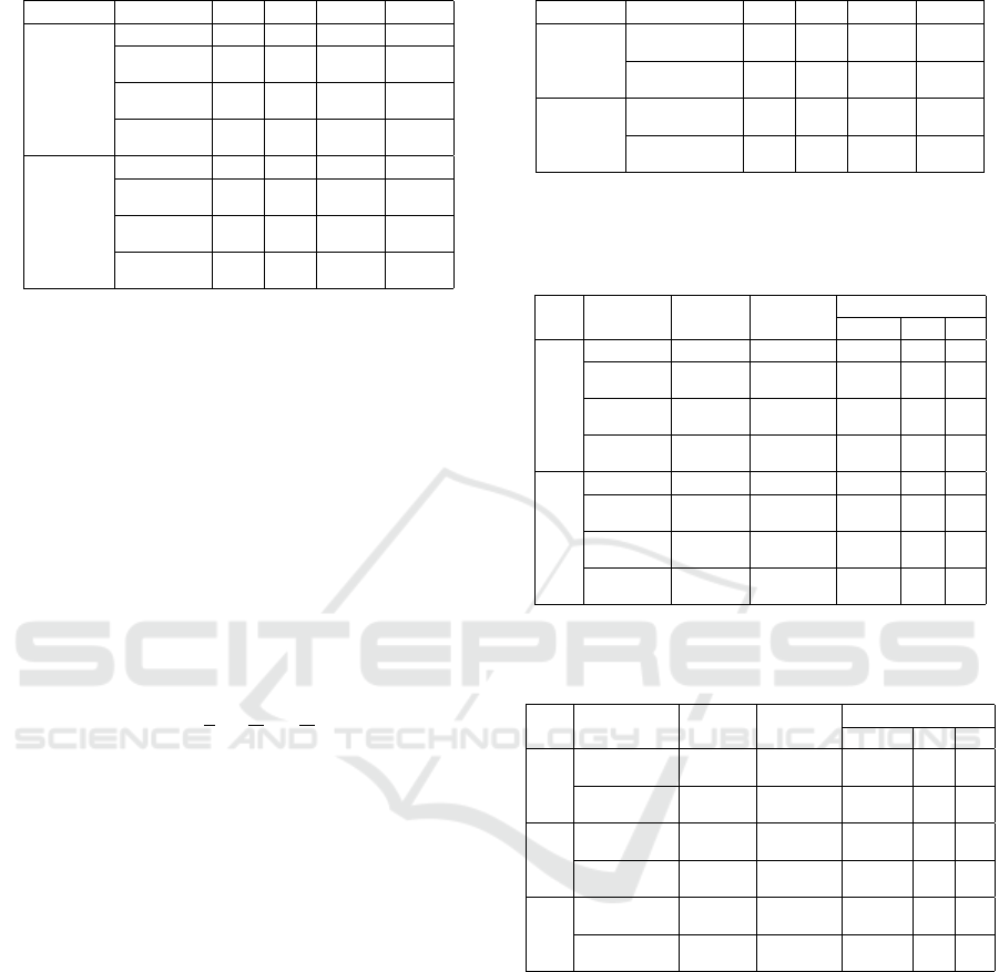
Table 1: Solved problems (Open-LR, Agents).
Vertex cost Alg. \|A| 2 4 6 8 10 12 14 16
5 sum-sum 1 1 1 1 1 1 1 0
max-sum 1 1 1 1 1 1 0 0
max-sum-l* 1 1 1 0
ms-sum 1 1 1 1 1 1 1 0
ms-sum-l* 1 1 1 0
lxm-sum 1 1 1 1 1 1 1 0
lxm-sum-l* 1 1 1 0
10 sum-sum 1 1 1 1 1 1 1 0
max-sum 1 1 1 1 1 1 0 0
max-sum-l* 1 1 1 0
ms-sum 1 1 1 1 1 1 1 0
ms-sum-l* 1 1 1 0
lxm-sum 1 1 1 1 1 0 0 0
lxm-sum-l* 1 0 0 0
* -l: limitation of CT with (c
cnst
, b
depth
, b
radix
)=(2, 16, 1.25) for
|A| ≥ 10.
• vlxm-vlxm: Vleximax for the cost values among
vertices in all agents’ paths.
Several methods employ additional techniques to
limit the size of search spaces, and those parameters
are also presented in the results.
We evaluated the number of solved instances by
the solvers. For solved instances, the numbers of ex-
panded nodes in the CBS algorithm, including the A*
algorithm in its low-level layer, were evaluated. For
the solution quality, we evaluated the SoC, makespan
and the Theil index (Matsui et al., 2018b), which is
a measurement of inequality. For n objectives, Theil
index T is defined as
T =
1
n
∑
i
v
i
¯v
log
v
i
¯v
(5)
where v
i
is the utility/cost value of an objective and ¯v
is the mean value for all of the objectives. The Theil
index takes a value in [0, logn]. If all utility/cost val-
ues are identical, the Theil index takes zero. Inequal-
ities based on different numbers of members can be
compared using population independence. We note
that the minimization of the leximin criterion does not
precisely minimize inequality, but rather is employed
as a tool to analyze the results.
Except for the case of Open-LR shown in Fig-
ure 3, the results were averaged over ten instances for
each problem setting by randomly assigning initial lo-
cations of agents within the limitations of the settings.
The results were aggregated for the instances whose
all trials were completed. We performed the experi-
ment on a computer with g++ (GCC) 8.5.0 -O3, Linux
4.18, Intel (R) Core (TM) i9-9900 CPU @ 3.10 GHz,
and 64 GB memory.
4.2 Results
Tables 1 and 2 show the number of solved problems
for the case of Open-LR. Here, we mainly concen-
Table 2: Solved problems (Open-LR, Vertices).
vertex cost alg. \|A| 2 4 6 8 10 12 14 16
5 vms-vms-lt* 1 0 0 0 0 0 0 0
vms-vms-lp* 1 1 1 1 1 1 1 0
vlxm-vlxm-lt* 1 0 0 0 0 0 0 0
vlxm-vlxm-lp* 1 1 1 1 1 1 0 0
10 vms-vms-lt* 1 0 0 0 0 0 0 0
vms-vms-lp* 1 1 1 1 1 1 1 0
vlxm-vlxm-lt* 1 0 0 0 0 0 0 0
vlxm-vlxm-lp* 1 1 1 1 1 1 0 0
* -lt: limitation of CT and the total path length without the
proportional constraint (c
cnst
, c
dist
, b
depth
, b
radix
)=(2, 2, 0, 2), -lp:
limitation of CT and the total path length with proportional constraint
using the same parameter.
Table 3: Expanded nodes (Open-LR, Agents, 10 agents).
Vertex Alg. #CT nodes #constraints #A* nodes processed
cost expanded of best slt. Total Ave. Max.
5 sum-sum 3871 13 1186931 305.9 700
max-sum 4017 13 1449448 360.0 706
max-sum-l* 4017 13 1449448 360.0 706
ms-sum 787 13 258205 324.4 639
ms-sum-l* 787 13 258205 324.4 639
lxm-sum 23013 13 8363639 363.3 706
lxm-sum-l* 10273 13 4327912 365.3 706
10 sum-sum 1265 10 786986 617.7 1121
max-sum 543 9 358693 649.8 1121
max-sum-l* 543 9 358693 649.8 1121
ms-sum 749 10 496742 655.3 1121
ms-sum-l* 749 10 496742 655.3 1121
lxm-sum 3207 9 2325004 722.9 1131
lxm-sum-l* 2571 9 1895327 710.9 1131
* -l: limitation of CT with (c
cnst
, b
depth
, b
radix
)=(2, 16, 1.25) for
|A| ≥ 10.
Table 4: Expanded nodes (Open-LR, Vertices, 10 agents).
Vertex Alg. #CT nodes #constraints #A* nodes processed
cost expanded of best slt. Total Ave. Max.
1 vms-vms-lt* 3749 10 213346 56.8 80
vms-vms-lp* 6653 10 352260 52.9 72
vlxm-vlxm-lt* 3749 10 213346 56.8 80
vlxm-vlxm-lp* 6653 10 352260 52.9 72
5 vms-vms-lt*
vms-vms-lp* 24821 11 2508100 100.2 138
vlxm-vlxm-lt*
vlxm-vlxm-lp* 83820 12 11770645 100.7 134
10 vms-vms-lt*
vms-vms-lp* 57397 9 6180128 106.1 139
vlxm-vlxm-lt*
vlxm-vlxm-lp* 69593 12 9244360 98.9 140
* -lt: limitation of CT and the total path length without the
proportional constraint (c
cnst
, c
dist
, b
depth
, b
radix
)=(2, 2, 0, 2), -lp:
limitation of CT and the total path length with proportional constraint
using the same parameter.
trated on the settings that can be solved by a tra-
ditional method using SoC. We limited the solution
methods based on a safeguard within the number of
5 × 10
5
CT nodes and 500 time steps for actions. In
addition, the execution of several instances was ter-
minated at the cut-off time of five minutes. In the
results, we employed the additional methods to limit
search spaces for several sizes of the problems. The
blank cells in the tables represent that the experiment
was omitted for small sizes of problems or relatively
large-scale problems could not be solved.
ICAART 2025 - 17th International Conference on Agents and Artificial Intelligence
230

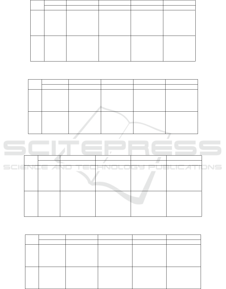
Table 5: Solution quality (Open-LR, Agents).
Vertex |A| 6 8 10 12
cost Alg. SoC MS Th SoC MS Th SoC MS Th SoC MS Th
5 sum-sum 108 21 0.011 149 21 0.009 193 22 0.011 245 25 0.012
max-sum 108 21 0.011 149 21 0.009 193 22 0.011 245 25 0.012
max-sum-l* 193 22 0.011 245 25 0.012
ms-sum 108 21 0.011 149 21 0.009 193 22 0.011 245 25 0.012
ms-sum-l* 193 22 0.011 245 25 0.012
lxm-sum 108 21 0.011 149 21 0.009 193 22 0.011 248 25 0.009
lxm-sum-l* 193 22 0.011 248 25 0.009
10 sum-sum 197 37 0.012 274 39 0.011 355 41 0.012 450 47 0.014
max-sum 197 37 0.012 274 39 0.011 355 41 0.012 455 46 0.012
max-sum-l* 355 41 0.011 455 46 0.012
ms-sum 197 37 0.012 274 39 0.011 355 41 0.012 455 46 0.012
ms-sum-l* 355 41 0.012 455 46 0.012
lxm-sum 197 37 0.012 274 39 0.011 355 41 0.011
lxm-sum-l* 355 41 0.011
* -l: limitation of CT with (c
cnst
, b
depth
, b
radix
)=(2, 16, 1.25) for |A| ≥ 10.
Table 6: Solution quality (Open-LR, Vertices).
Vertex |A| 6 8 10 12
cost Alg. SoC MS Th SoC MS Th SoC MS Th SoC MS Th
5 sum-sum 108 5 0.185 149 5 0.175 193 5 0.158 245 5 0.149
max-sum 108 5 0.185 149 5 0.175 193 5 0.158 245 5 0.149
vms-vms-lt*
vms-vms-lp* 116 5 0.175 161 5 0.163 209 5 0.146 260 5 0.132
vlxm-vlxm-lt*
vlxm-vlxm-lp* 117 5 0.175 166 5 0.160 214 5 0.148 273 5 0.135
10 sum-sum 197 10 0.231 274 10 0.229 355 10 0.204 450 10 0.195
max-sum 197 10 0.231 285 10 0.228 355 10 0.204 455 10 0.198
vms-vms-lt*
vms-vms-lp* 211 10 0.226 301 10 0.200 385 10 0.181 482 10 0.168
vlxm-vlxm-lt*
vlxm-vlxm-lp* 212 10 0.229 302 10 0.204 392 10 0.188 501 10 0.167
* -lt: limitation of CT and the total path length without the proportional constraint (c
cnst
, c
dist
, b
depth
, b
radix
)=(2, 2, 0, 2), -lp: limitation of CT and the
total path length with proportional constraint using the same parameter.
Table 7: Solution quality (Warehouse, Agents).
Vertex |A| 4 6 8 10
cost Alg. SoC MS Th SoC MS Th SoC MS Th SoC MS Th
5 sum-sum 65.7 24.2 0.097 107.7 27.4 0.078 147.9 27.7 0.075
max-sum 65.7 24.2 0.097 109.7 26.9 0.074 149.7 27 0.070
max-sum-l* 200.6 29 0.082
ms-sum 65.7 24.2 0.097 109.3 26.9 0.075 149.1 27 0.070
ms-sum-l* 198.1 29 0.083
lxm-sum 65.7 24.2 0.097 109.6 26.9 0.074 149.2 27 0.069
lxm-sum-l* 198.8 29 0.081
10 sum-sum 122 45.7 0.101 198.5 50.5 0.078 272.8 50.8 0.073
max-sum 123.8 45.1 0.097 202.2 48.8 0.073 274.6 49.7 0.068
max-sum-l* 366.6 54.1 0.081
ms-sum 123.8 45.1 0.097 201.7 48.8 0.073 273.8 49.7 0.068
ms-sum-l* 365.1 54.1 0.082
lxm-sum 123.8 45.1 0.097 203.6 48.8 0.070 277.5 49.7 0.067
lxm-sum-l* 367.2 54.1 0.079
* -l: limitation of CT with (c
cnst
, b
depth
, b
radix
)=(2, 16, 1.25) for |A| ≥ 10.
Table 8: Solution quality (Warehouse, Vertices).
Vertex |A| 2 4 6 8
cost Alg. SoC MS Th SoC MS Th SoC MS Th SoC MS Th
5 sum-sum 31 5 0.125 65.7 5 0.124 107.7 5 0.131 147.9 5 0.122
max-sum 31.5 5 0.128 65.7 5 0.124 109.7 5 0.132 149.7 5 0.126
vms-vms-lt* 31.2 5 0.125 65.9 5 0.123 108.5 5 0.140 148.6 5 0.127
vms-vms-lp* 31.1 5 0.121
vlxm-vlxm-lt* 32.1 5 0.126 67.6 5 0.125 115.6 5 0.139 159.7 5 0.125
vlxm-vlxm-lp* 31.2 5 0.117
10 sum-sum 57.5 9.4 0.161 122 9.3 0.154 198.5 9.7 0.167 272.8 9.9 0.161
max-sum 58.4 9.4 0.168 123.8 9.3 0.161 202.2 9.7 0.181 274.6 10 0.164
vms-vms-lt* 128.7 9.1 0.157 206.4 9.3 0.176 289.1 9.5 0.156
vms-vms-lp*
vlxm-vlxm-lt* 130.4 9.2 0.155 219.6 9.3 0.177
vlxm-vlxm-lp* 57.5 9.4 0.149
* -lt: limitation of CT and the total path length without the proportional constraint (c
cnst
, c
dist
, b
depth
, b
radix
)=(2, 2, 0, 2), -lp: limitation of CT and the
total path length with proportional constraint using the same parameter.
Investigation of MAPF Problem Considering Fairness and Worst Case
231

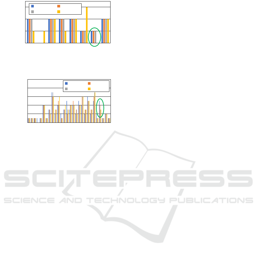
0
1
2
3
15 17 19 20 21 22 23 25
#Cost
Cost of Agents
sum-sum max-sum
ms-sum lxm-sum
Figure 4: Solution quality (Open-LR, Agents) (12 agents,
vertex cost = 5).
0
0.2
0.4
0.6
0.8
1
1 5 8 10 12 14 16 18 20 22 24 26 28 30
#Cost
Cost of Agents
sum-sum max-sum
ms-sum lxm-sum
Figure 5: Solution quality (Warehouse, Agents) (8 agents,
vertex cost = 5).
While the methods with a conventional criterion
found solutions in the relatively easy settings, several
settings were difficult for the leximax-based meth-
ods, which reveals the necessity of appropriate tech-
niques to effectively exclude unpromising solutions
from search spaces. In several results, the suitable
limitation of search space increased the success cases
of the search.
Tables 3 and 4 show the number of expanded
nodes in search processes for the case of Open-LR.
In both the high- and low-level searches, the size of
the searched space for leximax variants is generally
greater than the cases of traditional optimization crite-
ria. Although this additional computational cost is in-
herent in the specific criterion that considers fairness,
the result revealed the poor compatibility between
the leximax variants and the best-first search methods
without any limitation on search spaces. While the
criteria of leximax and vleximax required additional
computation to operate sorted objective vectors, that
was acceptable in comparison to the serious situations
of the excessive expansion of CT nodes.
In our preliminary experiment, the limitation to
winding paths in low-level search often locally in-
consistent with desired moves avoiding/waiting other
agents’ paths due to the limited length and the con-
straint to keep some tension of paths. Although this
situation is not the case of the optimization among
agents’ paths, it specifically deteriorated the results
of the optimization with vleximax. This revealed the
necessity of further investigation for more flexible re-
striction of the paths by considering the interaction
among agents having different lengths of paths.
In the high-level search, the best-first search of the
pure CBS algorithm that is not aware of the relation-
ship among the inserted constraints and their resulting
paths often expanded unpromising CT nodes. There-
fore, the search trees which is limited by some simple
strategies of beam search is often filled by such CT
nodes. To address this situation, more sophisticated
versions, in which both levels of search cooperate,
should be applied to this class of problems.
Tables 5-8 show the solution quality among differ-
ent optimization criteria. Since leximax and maxsum
are variants of ‘max’, the maximum cost value is the-
oretically identical. However, we employed a certain
limitation on the search space for leximax and max-
sum, and excessive settings of this limitation reduced
the characteristics of the criteria. In well-controlled
cases of the optimization among agents’ paths, the
leximax variants reduced the number of maximum
cost values by compromising on the total cost value.
Consequently, the Theil index values were relatively
decreased with the leximax variants. In the results of
the optimization among the agents’ paths, the maxi-
mum cost values were almost identical in most prob-
lem settings. In particular, the case of open grid with
relatively fewer number of agents appeared to reduce
the opportunities of difference of results.
In several cases of the optimization among agents’
paths, leximax criterion reduced the number of higher
cost values in objective vectors. Figures 4 and 5 show
the cases of the optimization among agents’ paths,
where leximin criterion worked in accordance with its
theoretical property.
However, in the case of the optimization among
path elements (i.e., vertices’ costs), the results by
vleximax revealed the difficulty of tuning the search.
When the optimization criteria of leximin variants are
affected by some disturbance in search processes, that
often fail to handle the worst case cost values. As a
result, this can totally increase cost values, including
the worst value, although the fairness among the cost
values is relatively preserved.
Regarding the scalability, the complete algorithms
are not so promising for large-scale problems, and
those methods are often employed to evaluate rel-
atively small problems in prototyping steps of new
classes of extended problems. Although we followed
this manner as the first study, the result revealed the
incompatibility of vleximax criterion with the solu-
tion methods based on simple best-first search.
A possible approach might employ appropriate
bounds of search space by referring the result of the
standard summation criterion and performs dedicated
ICAART 2025 - 17th International Conference on Agents and Artificial Intelligence
232

search strategies to efficiently cover the bounded
search space. Opportunities might also exist to em-
ploy local search methods that start from reasonable
initial solutions based on other optimization criteria
and find better solutions improving fairness and the
worst case.
5 CONCLUSIONS
We investigated multiagent pathfinding problems that
improve both fairness and the worst case among mul-
tiple objective values involving individual agents or
facilities. In the study, we applied variants of the
leximax criterion to MAPF problems and evaluated
this method with extended versions of the CBS al-
gorithm. The results revealed issues in controlling
a search with the leximax variants at both levels of
CBS when employing best-first search, while some
effect of the criterion was obtained in the optimiza-
tion among agents’ paths.
Although we addressed the case with the CBS al-
gorithm as a standard approach in our first study, the
result revealed several issues regarding the incom-
patibility between the vleximax criterion and simple
best-first search methods. As discussed in the pre-
vious section, opportunities might exist to additional
extension to more appropriately guide the best-first
search by considering the relationship among agent’s
paths and the cooperation of high- and low- level
search methods. The results might also suggest that
this kind of criterion is more compatible with other
approaches, including incomplete solution methods.
Partially greedy approaches such as variants of the
CA* algorithm or local search methods, rather than
comprehensive methods based on a fully best-first ap-
proach, also should be addressed. Our future work
will address an investigation in this direction as well
as analysis in more practical problem domains. While
we concentrated on the comparison of a few optimiza-
tion criteria as the first study, more extensive survey
regarding relating classes of MAPF/planning prob-
lems will also be included in our future work.
ACKNOWLEDGEMENTS
This study was supported in part by The Public
Foundation of Chubu Science and Technology Center
(thirty-third grant for artificial intelligence research)
and JSPS KAKENHI Grant Number 22H03647.
REFERENCES
Andreychuk, A., Yakovlev, K., Boyarski, E., and Stern, R.
(2021). Improving Continuous-time Conflict Based
Search. In Proceedings of The Thirty-Fifth AAAI Con-
ference on Artificial Intelligence, volume 35, pages
11220–11227.
Andreychuk, A., Yakovlev, K., Surynek, P., Atzmon, D.,
and Stern, R. (2022). Multi-agent pathfinding with
continuous time. Artificial Intelligence, 305:103662.
Barer, M., Sharon, G., Stern, R., and Felner, A. (2014).
Suboptimal Variants of the Conflict-Based Search Al-
gorithm for the Multi-Agent Pathfinding Problem. In
Proceedings of the Annual Symposium on Combinato-
rial Search, pages 19–27.
Barto, A. G., Bradtke, S. J., and Singh, S. P. (1995). Learn-
ing to act using real-time dynamic programming. Ar-
tificial Intelligence, 72(1-2):81–138.
Bouveret, S. and Lema
ˆ
ıtre, M. (2009). Computing leximin-
optimal solutions in constraint networks. Artificial In-
telligence, 173(2):343–364.
De Wilde, B., Ter Mors, A. W., and Witteveen, C. (2014).
Push and rotate: A complete multi-agent pathfinding
algorithm. J. Artif. Int. Res., 51(1):443–492.
Greco, G. and Scarcello, F. (2013). Constraint satisfaction
and fair multi-objective optimization problems: Foun-
dations, complexity, and islands of tractability. In Pro-
ceedings of the Twenty-Third International Joint Con-
ference on Artificial Intelligence, pages 545–551.
Hart, P., N. N. and Raphael, B. (1968). A formal basis
for the heuristic determination of minimum cost paths.
IEEE Trans. Syst. Science and Cybernetics, 4(2):100–
107.
Hart, P., N. N. and Raphael, B. (1972). Correction to ’a for-
mal basis for the heuristic determination of minimum-
cost paths’. SIGART Newsletter, (37):28–29.
Luna, R. and Bekris, K. E. (2011). Push and swap: Fast
cooperative path-finding with completeness guaran-
tees. In Proceedings of the Twenty-Second Interna-
tional Joint Conference on Artificial Intelligence, vol-
ume 1, pages 294–300.
Ma, H., Harabor, D., Stuckey, P. J., Li, J., and Koenig, S.
(2019). Searching with consistent prioritization for
multi-agent path finding. In Proceedings of the Thirty-
Third AAAI Conference on Artificial Intelligence and
Thirty-First Innovative Applications of Artificial In-
telligence Conference and Ninth AAAI Symposium on
Educational Advances in Artificial Intelligence, pages
7643–7650.
Ma, H., Li, J., Kumar, T. S., and Koenig, S. (2017). Lifelong
Multi-Agent Path Finding for Online Pickup and De-
livery Tasks. In Proceedings of the Sixteenth Confer-
ence on Autonomous Agents and MultiAgent Systems,
pages 837–845.
Marler, R. T. and Arora, J. S. (2004). Survey of
multi-objective optimization methods for engineer-
ing. Structural and Multidisciplinary Optimization,
26:369–395.
Matsui, T. (2019). A Study of Joint Policies Consider-
ing Bottlenecks and Fairness. In Proceedings of the
Investigation of MAPF Problem Considering Fairness and Worst Case
233

Eleventh International Conference on Agents and Ar-
tificial Intelligence, volume 1, pages 80–90.
Matsui, T., Matsuo, H., Silaghi, M., Hirayama, K., and
Yokoo, M. (2018a). Leximin asymmetric multiple
objective distributed constraint optimization problem.
Computational Intelligence, 34(1):49–84.
Matsui, T., Silaghi, M., Hirayama, K., Yokoo, M., and Mat-
suo, H. (2018b). Study of route optimization consid-
ering bottlenecks and fairness among partial paths. In
Proceedings of the Tenth International Conference on
Agents and Artificial Intelligence, pages 37–47.
Matsui, T., Silaghi, M., Okimoto, T., Hirayama, K., Yokoo,
M., and Matsuo, H. (2018c). Leximin multiple objec-
tive dcops on factor graphs for preferences of agents.
Fundam. Inform., 158(1-3):63–91.
Miyashita, Y., Yamauchi, T., and Sugawara, T. (2023). Dis-
tributed planning with asynchronous execution with
local navigation for multi-agent pickup and delivery
problem. In Proceedings of the Twenty-Second Inter-
national Conference on Autonomous Agents and Mul-
tiagent Systems, page 914–922.
Okumura, K. (2023). LaCAM: search-based algorithm
for quick multi-agent pathfinding. In Proceedings of
the Thirty-Seventh AAAI Conference on Artificial In-
telligence and Thirty-Fifth Conference on Innovative
Applications of Artificial Intelligence and Thirteenth
Symposium on Educational Advances in Artificial In-
telligence, pages 11655–11662.
Okumura, K., Machida, M., D
´
efago, X., and Tamura, Y.
(2022). Priority Inheritance with Backtracking for It-
erative Multi-Agent Path Finding. Artificial Intelli-
gence, 310.
Russell, S. and Norvig, P. (2003). Artificial Intelligence: A
Modern Approach (2nd Edition). Prentice Hall.
Sen, A. K. (1997). Choice, Welfare and Measurement. Har-
vard University Press.
Sharon, G., Stern, R., Felner, A., and Sturtevant, N. R.
(2015). Conflict-Based Search for Optimal Multi-
Agent Pathfinding. Artificial Intelligence, 219:40–66.
Silver, D. (2005). Cooperative Pathfinding. In Proceedings
of the AAAI Conference on Artificial Intelligence and
Interactive Digital Entertainment, pages 117–122.
Wang, F., Zhang, H., Koenig, S., and Li, J. (2024). Ef-
ficient approximate search for multi-objective multi-
agent path finding. In Proceedings of the Thirty-fourth
International Conference on Automated Planning and
Scheduling, pages 613–622.
Weise, J., Mai, S., Zille, H., and Mostaghim, S. (2020). On
the scalable multi-objective multi-agent pathfinding
problem. In Proceedings of the 2020 IEEE Congress
on Evolutionary Computation, pages 1–8.
Yakovlev, K. S. and Andreychuk, A. (2017). Any-angle
pathfinding for multiple agents based on SIPP al-
gorithm. In Proceedings of the Twenty-Seventh In-
ternational Conference on Automated Planning and
Scheduling, pages 586–593.
ICAART 2025 - 17th International Conference on Agents and Artificial Intelligence
234