Shape from Mirrored Polarimetric Light Field

Shunsuke Nakagawa

, Takahiro Okabe

3 a

and Ryo Kawahara

2 b

Department of Artiﬁcial Intelligence, Kyushu Institute of Technology, 680-4 Kawazu, Iizuka, Fukuoka 820-8502, Japan

Graduate School of Informatics, Kyoto University, Yoshida-honmachi, Sakyo-ku, Kyoto, 606-8501, Japan

Information Technology Track, Faculty of Engineering, Okayama University, 3-1-1 Tsushima-naka, Kita-ku, Okayama

700-8530, Japan

Keywords:

3D Shape Reconstruction, Polarization, Mirror.

Abstract:

While mirror reﬂections provide valuable cues for vision tasks, recovering the shape of mirror-like objects re-

mains challenging because they reﬂect their surroundings rather than displaying their own textures. A common

approach involves placing reference objects and analyzing their reﬂected correspondences, but this often intro-

duces depth ambiguity and relies on additional assumptions. In this paper, we propose a uniﬁed framework that

integrates polarization and geometric transformations for shape estimation. We introduce a 9-dimensional po-

larized ray representation, extending the Pl

ucker coordinate system to incorporate the polarization properties

of light as deﬁned by the plane of its electric ﬁeld oscillation. This enables the seamless evaluation of polar-

ized ray agreement within a homogeneous coordinate system. By analyzing the constraints of polarized rays

before and after reﬂection, we derive a method for per-pixel shape estimation. Our experimental evaluations

with synthetic and real images demonstrate the effectiveness of our method qualitatively and quantitatively.

1 INTRODUCTION

Recovering the shape of objects with perfectly mir-

ror surfaces is challenging, as these objects reﬂect

surrounding scenes rather than showing their inher-

ent textures. The robust solution has a wide range of

applications in product inspection, robotics, and ex-

tended reality (XR). Moreover, by leveraging the rich

visual information reﬂected on the surface, the rays

observable through a mirror contribute to wide-ﬁeld-

of-view shape recovery, precise localization, and efﬁ-

cient navigation.

In conventional studies, the shape cue of a

mirrored object is extracted by placing a texture-

referencing object, such as a display, and capturing

its reﬂection with a camera. However, even if a cor-

respondence is provided between the reference object

and the camera, ambiguity about the object’s shape

remains because its depth is not uniquely determined.

Therefore, assuming the surface integrability or lever-

aging the compound mirror’s ﬂatness is required for

shape recovery (Takahashi et al., 2012).

Polarization provides a clue to resolving this am-

biguity. The polarization before and after specular re-

https://orcid.org/0000-0002-2183-7112

https://orcid.org/0000-0002-9819-3634

ﬂection varies depending on the surface normal of the

object, allowing the normal to be recovered by utiliz-

ing multiple viewpoints (Miyazaki et al., 2012; Han

et al., 2024) or the unique polarization pattern of the

sky (Ichikawa et al., 2021). Lu et al. (Lu et al., 2019)

proposed an approach to reconstructing complex mir-

ror surfaces utilizing the polarization ﬁeld generated

by an LCD with one polarizing plate removed. How-

ever, it is necessary to use two or more calibrated po-

larized states of the liquid crystal, and the process ad-

ditionally requires the extra step of attaching and de-

taching the polarizing plates.

In previous methods, the geometry of correspond-

ing points and the constraints imposed by polariza-

tion are often treated independently or as separate

steps. Additionally, in polarization-based methods,

orthographic projection is typically assumed and re-

cently extended to perspective projection models (Pis-

tellato and Bergamasco, 2024). Can a framework be

established that describes the geometric transforma-

tion of both within a uniﬁed analysis in 3D space?

If achieved, this could naturally integrate the two

modalities to provide a structured approach to ana-

lyzing solution spaces.

In this paper, we show that the geometrical trans-

formation before and after reﬂection can be repre-

790

Nakagawa, S., Okabe, T. and Kawahara, R.

Shape from Mirrored Polarimetric Light Field.

DOI: 10.5220/0013389800003912

Paper published under CC license (CC BY-NC-ND 4.0)

In Proceedings of the 20th International Joint Conference on Computer Vision, Imaging and Computer Graphics Theory and Applications (VISIGRAPP 2025) - Volume 2: VISAPP, pages

790-796

ISBN: 978-989-758-728-3; ISSN: 2184-4321

sented using a 9-dimensional polarized ray. Speciﬁ-

cally, we extend the representation of light rays in the

ucker coordinate system by geometrically deﬁning

the properties of linearly polarized light as the normal

to the oscillation plane of the electric ﬁeld. Addition-

ally, we derive constraints for shape estimation from

the polarized rays before and after reﬂection. We en-

able a straightforward evaluation of the agreement be-

tween polarized rays by utilizing a homogeneous co-

ordinate system, and we formulate shape recovery as

a nonlinear optimization problem.

Our main contributions are as follows:

• Introducing the polarization light ﬁeld, which ex-

tends the conventional light ﬁeld by incorporating

the plane of polarization normals and demonstrat-

ing that polarization rays can be handled through

geometric transformations.

• Proposing a method for estimating the normal of a

mirror surface object for each pixel by leveraging

the reﬂection relationships of polarized rays.

2 RELATED WORK

Numerous studies have obtained the normal and posi-

tion of the mirror surface from the reference point and

its observation. In particular, in studies that focus on

planar mirrors (Sturm and Bonfort, 2006; Rodrigues

et al., 2010; Kumar et al., 2008), it is possible to re-

cover the mirror surface even when the pose of the ref-

erence object is unknown. Takahashi et al. (Takahashi

et al., 2012) leveraged multiple reﬂections to recover

the normal of a multi-facet mirror from two or more

corresponding points. On the other hand, since the

normal of the curved mirror differs for each pixel, not

only is a dense set of corresponding points required

but also steps, such as moving the reference (Kutu-

lakos and Steger, 2008; Grossberg and Nayar, 2005;

Liu et al., 2011; Han et al., 2021), are required to ob-

tain multiple constraints. Thus making it challenging

to cover a wide range of objects’ surfaces.

Some methods deal with the mirror surfaces by

adding additional constraints, such as the integrability

of the surface or radiometric clues (Liu et al., 2013;

Chari and Sturm, 2013). There are methods that use

LCDs as sources of polarized light (Lu et al., 2019;

Kawahara et al., 2023). These techniques take advan-

tage of polarization constraints through higher-order

nonlinear optimization problems, and the geometric

transformation relationships of polarization still re-

quire further exploration.

Shape from polarization (SfP), which reconstructs

normals based on polarization, has been studied ex-

tensively for dielectric materials. Some SfP methods

use specular reﬂection of unpolarized light as a clue

for estimating the normal. However, there is ambigu-

ity in the estimation (Atkinson and Hancock, 2006;

Miyazaki et al., 2003), so SfP also leverages addi-

tional clues such as multi-view (Cui et al., 2017; Zhao

et al., 2020) and shading(Smith et al., 2016; Huynh

et al., 2010) and active lighting (Ma et al., 2007;

Ichikawa et al., 2023).

While monocular SfP focuses on recovering sur-

face normals, our approach geometrically uniﬁes and

analyzes both the dense feature point correspon-

dences on the reference object and the polarization

correspondences, enabling simultaneous depth recov-

ery.

3 BASICS: POLARIZATION

Light is an electromagnetic wave that oscillates per-

pendicularly to the direction of propagation. The os-

cillation plane of light, invisible to the human eyes,

has random directions for sunlight or incandescent

lamps. This type of light is called unpolarized light.

In contrast, light from LCDs and other sources that

pass through linear polarizers has only a single oscil-

lation plane, and this type of light is called linearly

polarized light.

If we deﬁne a plane perpendicular to the direction

of light propagation, the amplitude of the electric ﬁeld

of linearly polarized light can be represented as a 2D

Jones vector ˇe as follows;

ˇe =







cosα

sinα



, (1)

where E

and E

are the x and y components of the

amplitude E

in the plane.

We can leverage polarizing ﬁlters to obtain the an-

gle α of the light oscillation in Eq. 1. A polarizing

ﬁlter extracts the polarization component at a speciﬁc

angle. Speciﬁcally, we place a polarizing ﬁlter in front

of the camera and calculate the polarization angle α

from the intensity captured at multiple known ﬁlter

angles ψ. The amplitude transmission of the electric

ﬁeld ˇe

(ψ) for a ﬁlter angle ψ can be described using

the Jones calculus as follows (Collett, 2005);

ˇe

(ψ) =



cos

ψ cosψsinψ

cosψ sinψ sin



ˇe

= E



cosψ cos(ψ − α)

sinψ sin(ψ − α)



(2)

When the energy of this electric ﬁeld is observed as

intensity by a camera, the following holds;

I(ψ) ∝ || ˇe

(ψ)||

. (3)

Shape from Mirrored Polarimetric Light Field

791

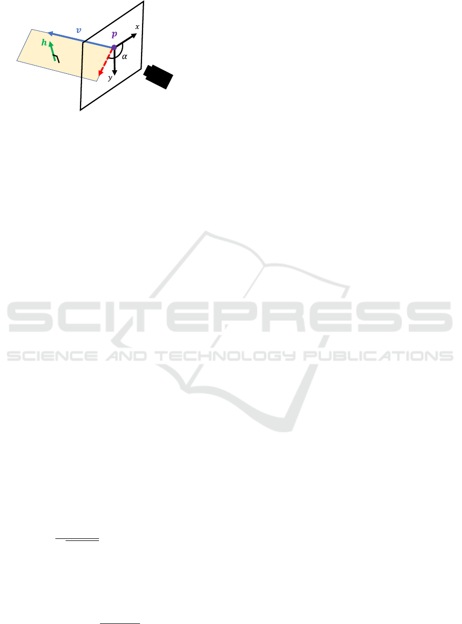
Image plane

Polarization camera

Plane of

polarization

Figure 1: Polarized Ray. The plane of polarization is

spanned by the direction of the electric ﬁeld and the view-

ing direction.

Therefore, from Eq. 2 and Eq. 3, when the ﬁlter angle

of the polarizing camera is ψ, linear polarization with

AoLP α is observed with an intensity of

I(ψ) = I

+ I

cos(2ψ − 2α). (4)

We can utilize a quad-Bayer polarization camera to

simultaneously obtain polarization images of four ﬁl-

ter angles ψ = (0,π/4,π/2, 3π/4) in a single shot and

recover the sinusoidal in Eq. 4 (Huynh et al., 2010).

4 METHOD

By extending the existing light ﬁeld representation,

we describe the transformation of both polarization

state and ray geometry and recover the shape of the

mirror object by analyzing it.

4.1 Polarimetric Light Field

The viewing direction vectors for each pixel form a

unique set of rays by mirror reﬂection. Let us de-

scribe the rays of the light ﬁeld by extending them

with polarization.

Polarized Ray. As shown in Fig. 1, The direction

vector of the electric ﬁeld at the image plane can be

described in 3D space, using AoP α obtained from the

observation as follows;

e =

+ E













cosα

sinα





. (5)

The plane of polarization (PoP) on which the electric

ﬁeld oscillates is spanned by e and the viewing di-

rection v

. Thus, we can represent PoP by its normal

h =

v × e

⊤

||v × e

⊤

(6)

Let us consider the expansion of the Pl

ucker coor-

dinates system (Sturm and Barreto, 2008) to evaluate

whether rays are equivalent. This 6D homogeneous

coordinate system can express arbitrary rays and con-

sists of two components: the direction of the ray v

and the normal δ of the plane spanned by the origin

and the ray, also called the moment.







o × v



∈ R

, (7)

where o denotes the origin of the ray, and v is a unit

vector. We combine this with the PoP in Eq. 5 to de-

ﬁne the polarized ray ℓ ∈ R

as follows.

ℓ =





o × v





. (8)

Note that there is a sign ambiguity in the normal vec-

tor that deﬁnes PoP.

Geometric Transformation. The coordinate trans-

formation is linear w.r.t. the direction of the ray ℓ,

the origin o, and the PoP direction h. Thus, the mir-

ror transformation can be described using the House-

holder matrix H and the translation vector t

as fol-

lows;

′

= Hv,

′

= Ho + t

′

= Hh,

(9)

where the H and t

are deﬁned by the mirror normal

n and the distance to the mirror plane d

H = I − 2nn

⊤

, t

= −2d

n. (10)

From Eq. 9, the mirror transformation of a polarized

ray ℓ can be described using a matrix M ∈ R

9×9

, as

follows;

ℓ

′

= Mℓ





H 0 0

× H H 0

0 0 H





ℓ.

(11)

Up to this point, we can geometrically transform the

polarized rays that consist of the polarized light ﬁeld.

4.2 Shape from Mirrored Polarimetric

Light Field

As shown in Fig. 2, suppose that the point p

on the

LCD is reﬂected on the object surface and observed in

the polarization camera’s viewing direction v

. The

goal is to obtain the object surface’s normal n and

depth z. We ﬁrst introduce the constraints for this

imaging system when all the other unknowns are ob-

tained.

VISAPP 2025 - 20th International Conference on Computer Vision Theory and Applications

792

Mirror

LCD

Polarization

camera

Figure 2: Shape from Mirrored Polarimetric Light Field.

Constraints. In summary, the constraint is that the

mirror transformation of the polarized light observed

by the camera matches the known polarized light de-

ﬁned on the display side. When the direction of the

electric ﬁeld e

is obtained in the viewing v

of the

polarization camera, the PoP normal h

is described

× e

⊤

||v

× e

⊤

. (12)

Thus, the polarized ray ℓ

obtained on the polarization

camera side is described as

ℓ





o × v





, (13)

where o is the camera’s origin. Also, the polarized

ray ℓ

is reﬂected at the object surface to become ℓ

′

ℓ

′

= Mℓ





× Hv





, (14)

On the other hand, polarized light can also be de-

scribed on the display side. When the corresponding

point on the LCD is p

and its electric ﬁeld direction

is e

in the camera coordinate system, the PoP normal

is described as

× e

⊤

||Hv

× e

⊤

. (15)

Therefore, the polarized ray ℓ

of the LCD side be-

comes

ℓ





× Hv





. (16)

Since these polarized rays are represented in ho-

mogeneous coordinates, ℓ

′

and ℓ

become identical.

Noting the ambiguity of the sign of the PoP normal,

we can obtain the constraints as

× Hv

− p

× Hv

= 0,

× h

= 0.

(17)

The degree of freedom (DOF) of the normal n is 2,

and the DOF of mirror plane distance d

is 1, but

Eq. 17 is nonlinear. Therefore, for robust estimation,

we introduce regularization that assumes the integra-

bility of the surface.

= ||1 − n

⊤

, (18)

where n

is the surface normal calculated using the

neighboring depth as

(−∂

z,−∂

z,1)

⊤

||(−∂

z,−∂

z,1)

⊤

(19)

Note that the depth z can be obtained by the mirror

plane distance d

and z-component of the viewing z

as z = d

. We deﬁne the following error function

from Eq. 17 to optimize together with Eq. 18,

= ||(t

− p

) × Hv

= ||Hh

× h

(20)

Finally, we consider the following minimization prob-

lem.

min

n,d

+ λ

), (21)

where λ

, λ

are the optimization weight.

Shape Estimation. To obtain the direction of the

electric ﬁeld e

from the polarization camera obser-

vations, we calculate the value of α in Eq. 4 for each

pixel in the captured image, and then apply to Eq. 5.

The direction of the electric ﬁeld of the LCD is known

as a product-speciﬁc angle in the image coordinate

system of the LCD (typically, it is either horizontal,

vertical, or π/4). Denoting the vector formed by ap-

plying this to Eq. 5 as ˆe

, then e

in the camera coor-

dinate system is calculated with the calibrated display

rotation R

= R

ˆe

. (22)

Regarding the point p

on the LCD corresponding

to the camera’s line of sight v

, we leverage existing

structured lighting to obtain the correspondence. De-

noting the corresponding point in the LCD’s local co-

ordinate system as ˆp

, the transformation to the cam-

era coordinate system is described as

= R

ˆp

+ t

, (23)

where t

is the translation vector of the display w.r.t.

the camera. Up to this point, we have obtained the

input for Eq. 21 to recover the shape through the opti-

mization.

Shape from Mirrored Polarimetric Light Field

793

(a) (b)

GT GTEstimated Error ErrorEstimated

W/o

polarization

Ours

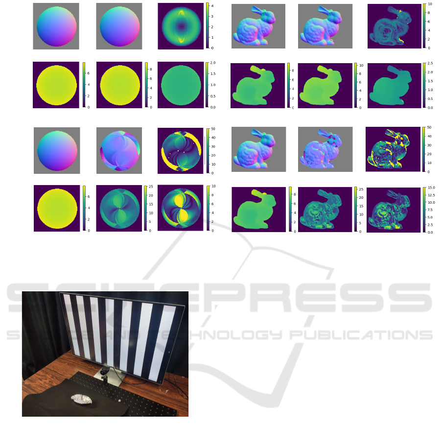
Figure 3: The shape reconstruction results with synthetic (a) Sphere and (b) Bunny data. The upper row of each method shows

the results of normal estimation, and the lower row shows the depth estimation results. The error maps of the normal are

calculated as an angular error in degree, and the error maps of the depth are in cm.

LCD

Object

Polarization

camera

Figure 4: Experimental Setup.

5 RESULTS

In this section, we evaluate our method’s prototyping

and demonstrate its effectiveness through quantitative

evaluation using synthetic data and reconstruction re-

sults using real images.

5.1 Quantitative Evaluation with

Synthetic Data

We quantitatively evaluate the accuracy of our re-

construction using synthetic data. We rendered the

simple-shaped Sphere and the complex-shaped Bunny

as target objects under a linear polarized light source.

Considering the actual environment, we set the dis-

tance from the camera to the object to be about 0.8

m and the size of the subject to be about 0.10 m. As

a baseline method, we compare to the approach that

does not utilize polarization (i.e. w/o E

Here, the initial value of the normal vector is set to

face the front, and the depth is set to 0.8 m as a plane.

We used Pytorch’s Adam optimizer for optimization

and set λ

= 1.0 and λ

= 100 for Eq. 21. The num-

ber of iterations for parameter updates was set to 700.

Regarding comparison methods, many SfP methods

assume an unpolarized light source and dielectric ma-

terial, which makes direct comparison difﬁcult.

Fig. 3 shows the experimental results of the syn-

thetic data. Although the shape obtained by our

method was qualitatively accurate compared to the

baseline method, an error can still be observed even

in the experiment without the intensity noise. These

results suggest that a local minimum exists in the op-

timization of Eq. 21. Speciﬁcally, the symmetric error

structure shown in Fig. 3(a) suggests a local minimum

that depends on the polarization direction of the dis-

play. This occurs when the optimization starts from

the initial value of the normal vector that we set uni-

formly oriented forward.

VISAPP 2025 - 20th International Conference on Computer Vision Theory and Applications

794

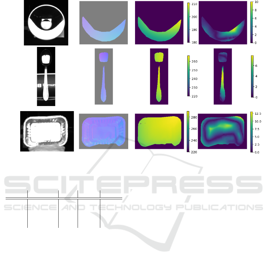
Input Normal Depth Depth error

(a)

(b)

(c)

Figure 5: The shape reconstruction results of real-world objects. (a) Elipse Mirror, (b) Spoon, (c) Aluminum cup. The error

of the depth map is in mm.

Table 1: Results of refractive index estimation.

Input Error Ours w/o E

w/o E

Sphere

Normal (

◦

) 0.74 0.87 8.15

Depth (m) 0.042 0.047 0.167

Bunny

Normal (

◦

) 2.62 2.99 13.31

Depth (m) 0.106 0.124 0.316

5.2 Ablation Study

For further evaluation of the optimization, we verify

the effect of the regularization term E

through abla-

tion experiments.

Table 1 shows the difference in results with and

without the regularization term E

and the PoP error

cost E

. These results show that the consistency of

depth and normals work as effective guidance even

for general shapes such as Bunny and that both nor-

mals and depth results are improved.

5.3 Real World Objects

As shown in Fig. 4, our system consist of a single

LCD (HUAWEI MateView 3840×2560px) and a sin-

gle polarization camera (FLIR BFS-U3-51S5P). The

relative pose of the LCD and the polarization camera

is calibrated beforehand using a planner mirror. We

used the same strategy as in the simulation experiment

in Sec. 5.1 for the initial normal and depth values. The

ground truth depth value in the evaluation is obtained

by aligning the depth camera (Intel RealSense D405)

values.

Fig. 5 shows that our method can successfully re-

cover the surface normals and depth of mirror objects

in the real world. These results qualitatively demon-

strate that both global and local shapes can be re-

covered. The average depth error are 2.84mm for

Elipse Mirror, 3.21mm for Spoon, and 4.25mm for

Aluminum cup, respectively. Note that the results only

show the areas that can be recovered, and this area

depends on the direction of the light source that the

display can illuminate.

6 CONCLUSION

In this paper, we introduce a novel method for recon-

structing the per-pixel surface normals and depths of

mirror objects. By analyzing the polarization light

ﬁeld formed by polarized rays described in a homo-

geneous coordinate system, we clarify the geomet-

ric constraints imposed by both. Our approach uni-

ﬁes polarization and geometry under a single analy-

sis, providing a structured and efﬁcient method for

reconstructing the shape of mirror surfaces. Exper-

Shape from Mirrored Polarimetric Light Field

795

imental results show that our method can accurately

reconstruct the per-pixel depths and surface normals

of various mirror surfaces. Our future work includes

extending the system to a polarized light source com-

bining a mirror and LCD and calibrating a catadiop-

tric system that handles polarization.

Limitations. The primary limitation of our method

is that the reconstructible area of the object is lim-

ited by the spatial range of the display’s illumination.

This issue could be mitigated by using multiple LCDs

or incorporating curved displays. Additionally, the

method assumes a metallic surface, which may re-

strict its applicability. This limitation could be ad-

dressed by extending the approach to handle dielectric

materials using Fresnel reﬂection.

ACKNOWLEDGEMENTS

This work was supported by JSPS KAKENHI Grant

Numbers JP20H00612 and JP22K17914.

REFERENCES

Atkinson, G. A. and Hancock, E. R. (2006). Recovery of

surface orientation from diffuse polarization. IEEE

TIP, 15(6):1653–1664.

Chari, V. and Sturm, P. (2013). A theory of refractive photo-

light-path triangulation. In CVPR, pages 1438–1445.

Collett, E. (2005). Field guide to polarization. Spie Belling-

ham.

Cui, Z., Gu, J., Shi, B., Tan, P., and Kautz, J. (2017). Polari-

metric multi-view stereo. In CVPR, pages 1558–1567.

Grossberg, M. D. and Nayar, S. K. (2005). The raxel imag-

ing model and ray-based calibration. IJCV, 61:119–

137.

Han, K., Liu, M., Schnieders, D., and Wong, K.-Y. K.

(2021). Fixed viewpoint mirror surface reconstruction

under an uncalibrated camera. IEEE TIP.

Han, Y., Guo, H., Fukai, K., Santo, H., Shi, B., Okura, F.,

Ma, Z., and Jia, Y. (2024). Nersp: Neural 3d recon-

struction for reﬂective objects with sparse polarized

images. In CVPR, pages 11821–11830.

Huynh, C. P., Robles-Kelly, A., and Hancock, E. (2010).

Shape and refractive index recovery from single-view

polarisation images. In CVPR, pages 1229–1236.

Ichikawa, T., Nobuhara, S., and Nishino, K. (2023). Spi-

ders: Structured polarization for invisible depth and

reﬂectance sensing. ArXiv, abs/2312.04553.

Ichikawa, T., Purri, M., Kawahara, R., Nobuhara, S., Dana,

K., and Nishino, K. (2021). Shape from sky: Polari-

metric normal recovery under the sky. In CVPR, pages

14832–14841.

Kawahara, R., Kuo, M.-Y. J., and Okabe, T. (2023). Po-

larimetric underwater stereo. In Scandinavian Con-

ference on Image Analysis, pages 534–550. Springer.

Kumar, R. K., Ilie, A., Frahm, J.-M., and Pollefeys, M.

(2008). Simple calibration of non-overlapping cam-

eras with a mirror. In CVPR, pages 1–7. IEEE.

Kutulakos, K. N. and Steger, E. (2008). A theory of refrac-

tive and specular 3d shape by light-path triangulation.

IJCV, 76:13–29.

Liu, M., Hartley, R., and Salzmann, M. (2013). Mirror sur-

face reconstruction from a single image. In CVPR.

Liu, M., Wong, K.-Y. K., Dai, Z., and Chen, Z. (2011).

Specular surface recovery from reﬂections of a pla-

nar pattern undergoing an unknown pure translation.

In ACCV, pages 137–147. Springer.

Lu, J., Ji, Y., Yu, J., and Ye, J. (2019). Mirror surface re-

construction using polarization ﬁeld. In ICCP, pages

1–9.

Ma, W.-C., Hawkins, T., Peers, P., Chabert, C.-F., Weiss,

M., Debevec, P. E., et al. (2007). Rapid acquisi-

tion of specular and diffuse normal maps from polar-

ized spherical gradient illumination. Rendering Tech-

niques, 9(10):2.

Miyazaki, D., Shigetomi, T., Baba, M., Furukawa, R.,

Hiura, S., and Asada, N. (2012). Polarization-based

surface normal estimation of black specular objects

from multiple viewpoints. In 2012 Second Interna-

tional Conference on 3D Imaging, Modeling, Process-

ing, Visualization and Transmission, pages 104–111.

Miyazaki, D., Tan, R. T., Hara, K., and Ikeuchi, K. (2003).

Polarization-based inverse rendering from a single

view. In ICCV, pages 982–982.

Pistellato, M. and Bergamasco, F. (2024). The raxel

imaging model and ray-based calibration. IJCV,

132:4688—-4702.

Rodrigues, R., Barreto, J. P., and Nunes, U. (2010). Camera

pose estimation using images of planar mirror reﬂec-

tions. In Daniilidis, K., Maragos, P., and Paragios, N.,

editors, ECCV, pages 382–395, Berlin, Heidelberg.

Springer Berlin Heidelberg.

Smith, W. A., Ramamoorthi, R., and Tozza, S. (2016). Lin-

ear depth estimation from an uncalibrated, monoc-

ular polarisation image. In ECCV, pages 109–125.

Springer.

Sturm, P. and Barreto, J. P. (2008). General imaging geom-

etry for central catadioptric cameras. In ECCV, pages

609–622. Springer.

Sturm, P. and Bonfort, T. (2006). How to compute the

pose of an object without a direct view? In ACCV,

ACCV’06, page 21–31, Berlin, Heidelberg. Springer-

Verlag.

Takahashi, K., Nobuhara, S., and Matsuyama, T. (2012). A

new mirror-based extrinsic camera calibration using

an orthogonality constraint. In 2012 IEEE Conference

on Computer Vision and Pattern Recognition, pages

1051–1058. IEEE.

Zhao, J., Monno, Y., and Okutomi, M. (2020). Polarimetric

multi-view inverse rendering. In ECCV, pages 85–

102. Springer.

VISAPP 2025 - 20th International Conference on Computer Vision Theory and Applications

796