Grid Cost Allocation in Peer-to-Peer Electricity Markets: Benchmarking

Classical and Quantum Optimization Approaches

David Bucher

1 a

, Daniel Porawski

, Benedikt Wimmer

, Jonas N

ußlein

2 b

, Corey O’Meara

3 c

Giorgio Cortiana

3 d

and Claudia Linnhoff-Popien

Aqarios GmbH, Prinzregentenstraße 120, 81677 Munich, Germany

Department for Computer Science, LMU Munich, Germany

E.ON Digital Technology GmbH, Hannover, Germany

{david.bucher, daniel.porawski}@aqarios.com,

ﬁ

{c m

Keywords:

Quantum Optimization, Quantum Annealing, Peer-to-Peer Markets, Benchmarking, Convex Optimization.

Abstract:

This paper presents a novel optimization approach for allocating grid operation costs in Peer-to-Peer (P2P)

electricity markets using Quantum Computing (QC). We develop a Quadratic Unconstrained Binary Opti-

mization (QUBO) model that matches logical power ﬂows between producer-consumer pairs with the physi-

cal power ﬂow to distribute grid usage costs fairly. The model is evaluated on IEEE test cases with up to 57

nodes, comparing Quantum Annealing (QA), hybrid quantum-classical algorithms, and classical optimization

approaches. Our results show that while the model effectively allocates grid operation costs, QA performs

poorly in comparison despite extensive hyperparameter optimization. The classical branch-and-cut method

outperforms all solvers, including classical heuristics, and shows the most advantageous scaling behavior. The

ﬁndings may suggest that binary least-squares optimization problems may not be suitable candidates for near-

term quantum utility.

1 INTRODUCTION

The increasing adoption of distributed energy re-

sources and the ongoing transformation of electricity

consumers into prosumers drive fundamental changes

in power systems operation. P2P electricity markets

have emerged as a promising paradigm to facilitate

direct energy trading between prosumers while main-

taining grid stability and operational efﬁciency (Sousa

et al., 2019). However, a key challenge in imple-

menting P2P markets lies in fairly allocating grid op-

eration costs among participants based on their ac-

tual infrastructure usage. Traditional constant net-

work tariffs become inadequate in P2P settings as

they fail to account for the complex power ﬂow

patterns that emerge from bilateral trades (Baroche

et al., 2019), leading to unfair cost distributions be-

tween customers. This requires dynamic cost allo-

https://orcid.org/0009-0002-0764-9606

https://orcid.org/0000-0001-7129-1237

https://orcid.org/0000-0001-7056-7545

https://orcid.org/0000-0001-8745-5021

cation mechanisms to appropriately distribute grid

operation and maintenance costs among market par-

ticipants based on their contribution to network uti-

lization. To implement P2P, the Distribution Sys-

tem Operator (DSO) requires that the cost allocation

mechanism covers all operational and maintenance

costs. The combinatorial nature of matching multiple

producers and consumers presents a computationally

challenging optimization problem.

QC, particularly Quantum Annealing (QA), has

shown promise in solving complex combinatorial op-

timization problems in various domains (Abbas et al.,

2024). Recent advances in quantum hardware and hy-

brid quantum-classical algorithms offer new opportu-

nities to address challenging energy sector optimiza-

tion problems (Blenninger et al., 2024). However, the

practical utility of quantum approaches for P2P mar-

ket optimization remains largely unexplored.

This paper makes two main contributions: First,

we develop a novel optimization model for allocat-

ing grid usage costs in P2P electricity markets based

on actual power ﬂow patterns. Second, we conduct

a comprehensive benchmark study comparing quan-

Bucher, D., Porawski, D., Wimmer, B., Nüßlein, J., O’Meara, C., Cortiana, G. and Linnhoff-Popien, C.

Grid Cost Allocation in Peer-to-Peer Electricity Markets: Benchmarking Classical and Quantum Optimization Approaches.

DOI: 10.5220/0013391400003890

Paper published under CC license (CC BY-NC-ND 4.0)

In Proceedings of the 17th International Conference on Agents and Artiﬁcial Intelligence (ICAART 2025) - Volume 1, pages 751-762

ISBN: 978-989-758-737-5; ISSN: 2184-433X

751

tum annealing, hybrid quantum-classical, and classi-

cal optimization approaches for solving the proposed

model. Our analysis provides insights into the poten-

tial and limitations of current quantum optimization

techniques for P2P market applications.

The remainder of this paper is organized as fol-

lows: Sec. 2 provides background on quantum an-

nealing and classical optimization and reviews related

work. Sec. 3 presents our problem formulation for

P2P cost allocation. Sec. 4 analyzes the model be-

havior through a detailed case study. Sec. 5 presents

benchmark results comparing different optimization

approaches, and Sec. 6 concludes, giving future re-

search directions.

2 BACKGROUND & RELATED

WORK

2.1 Quantum Annealing

The quantum bit (qubit), as the elementary informa-

tion unit in quantum mechanics, manifests in super-

position states |ψ⟩= α |0⟩+β|1⟩ with |α|

+|β|

= 1.

This property enables n coupled qubits to encode the

complete set of 2

bit conﬁgurations in a quantum

state described by

|ψ⟩ =

−1

∑

x=0

|x⟩, (1)

for x ∈ {0,1}

. Computational basis measurements

reveal bit string x with probability |ψ

(Nielsen and

Chuang, 2010), forming the foundation for quantum

optimization approaches that maximize the measure-

ment probability of optimal bit conﬁgurations.

The framework for quantum optimization typi-

cally employs an Ising Hamiltonian constructed from

Pauli z-matrices

= |0⟩⟨0|−|1⟩⟨1|. This cost oper-

ator takes the form

= −

∑

i, j

⊗

−

∑

, (2)

where tensor products indicate simultaneous opera-

tions on qubit pairs (i, j). The diagonality of

the z-basis ensures its ground state corresponds to

a computational basis state x

∗

. The classical repre-

sentation of bit string energies follows naturally as

⟨x|

|x⟩ = H

(x), yielding the QUBO formulation:

(x) = −

∑

i, j

−

∑

i, j

, (3)

with z

= 1−2x

and

⟩= z

⟩. This equivalence

enables physical implementation of the Ising Hamil-

tonian for combinatorial optimization (Lucas, 2014).

The solution methodology leverages the adiabatic the-

orem (Born and Fock, 1928; Farhi et al., 2001), which

postulates that a system maintains ground-state oc-

cupation under sufﬁciently slow Hamiltonian evo-

lution. Adiabatic Quantum Computing (AQC) ex-

ploits this principle by initializing the system in |+⟩=

−n/2

∑

|x⟩, the ground state of

= −

∑

. Time

evolution proceeds under

H(s) = s

+ (1 −s)

, (4)

with s ∈ [0,1]. Ideally, adiabatic evolution from s = 0

to s = 1 yields the QUBO solution state |x

∗

⟩.

Physical implementations, however, must contend

with decoherence and noise, necessitating accelerated

evolution times. This practical constraint transitions

the process from AQC to QA (Rajak et al., 2023).

While this departure from the adiabatic regime re-

duces the optimal state probability |ψ

∗

, repeated

measurements can still reveal the desired solution.

Hence, QA is considered approximate optimization.

Current QA hardware, exempliﬁed by D-Wave’s

Advantage System QPU, implements this approach

using over 5000 qubits interconnected by 35000 cou-

plers (McGeoch and Farr

e, 2021). The underlying

Pegasus topology establishes 15 couplings per qubit,

though this ﬁxed architecture introduces implemen-

tation challenges for problems requiring higher con-

nectivity. Such cases necessitate the embedding of

logical qubits as multiple physical qubits (so-called

chains).

In addition to its QPUs, D-Wave offers a propri-

etary cloud-based hybrid quantum solver (Leap). The

solver employs graph partitioning to decompose large

optimization problems into quantum-compatible sub-

problems, which are then solved through parallel pro-

cessing using both QA and classical algorithms. A

central orchestrator dynamically allocates these sub-

problems between quantum and classical resources

while a merging process reconstructs the complete

solution. This hybrid architecture enables handling

large-scale problems beyond quantum hardware lim-

itations while maintaining solution quality through

adaptive reﬁnement strategies (D-Wave, 2020).

2.2 Classical Solvers

Optimization heuristics produce fast solutions repeti-

tively to arrive at a reasonable solution candidate in-

stead of a structured search in the space of possible so-

lutions. Even though the optimal solution is often not

reachable for heuristics, the fast runtime and close-to-

optimal solutions are more desirable in many practi-

cal application scenarios, especially if exact methods

suffer from lengthy runtimes.

QAIO 2025 - Workshop on Quantum Artiﬁcial Intelligence and Optimization 2025

752

Simulated Annealing (SA) is a QUBO heuristic, a

Markov-Chain Monte Carlo method, that starts from a

random initial point and iteratively proposes bit-ﬂips

in its current solution (Kirkpatrick et al., 1983). If

a bit-ﬂip decreases cost, it will be accepted directly.

Still, when it increases, it will only be accepted based

on an acceptance probability dictated by the cost delta

and an annealing parameter β. This parameter in-

creases with every iteration, shifting the search strat-

egy from exploration to exploitation.

Tabu Search (TS) enhances the local search

method by maintaining a tabu list of recently explored

samples in memory to prevent cycling and escape lo-

cal optima (Glover, 1989). At each iteration, it eval-

uates the neighborhood of the current solution and

moves to the best non-tabu neighbor, even if this leads

to a temporary deterioration in solution quality.

Gurobi is a state-of-the-art classical branch-and-

cut solver that structurally explores the search space

using the branch-and-bound algorithm in conjunc-

tion with various cutting plane methods (Gurobi Op-

timization, 2024). Gurobi is capable of solving linear

programming as well as quadratic programming prob-

lems with various constraints.

2.3 Related Work

To the best of the authors’ knowledge, QC has not

been investigated to solve the problem of P2P Cost

Allocation directly, although several applications of

QC within the optimal use of energy exist. Speciﬁ-

cally, applications of QA to solve the problem of grid

partitioning use-cases (Fern

andez-Campoamor et al.,

2021; Colucci et al., 2023; Bucher et al., 2024b) have

successfully demonstrated some of these ﬁrst appli-

cations. Furthermore, gate-based optimization algo-

rithms showed promising results for applications in

load scheduling (Mastroianni et al., 2024), charging

optimization (Kea et al., 2023), and coalition forma-

tion (Mohseni et al., 2024). Finally, QA has been

applied for matching producer and consumer pairs in

P2P markets (O’Meara et al., 2023) without consider-

ing cost allocation.

P2P markets have been studied extensively in

the literature. Early work on P2P electricity mar-

kets focused primarily on bilateral trading mecha-

nisms where prosumers directly negotiate energy ex-

changes. Later work introduced a P2P energy trading

framework incorporating network constraints and dis-

tribution fees (Sousa et al., 2019). The challenge of

fair cost allocation gained prominence as researchers

recognized that traditional volumetric network tariffs

could lead to inefﬁcient market outcomes in P2P set-

tings. This study is based on modeling aspects de-

veloped by Baroche et al. (Baroche et al., 2019),

who applied cooperative game theory concepts like

the Shapley value to allocate network costs among

peers, and has been extended by incorporating net-

work losses and congestion costs in their allocation

framework (Le Cadre et al., 2020).

3 PROBLEM FORMULATION

A power grid can be described as a graph G(V,E)

with power lines as edges E and loads or genera-

tors as nodes i ∈ V = P ∪C, where P and C are

the sets of producers and consumers, respectively.

Given a self-reliant section of the power grid with

the nodal power injection d

balanced by the load,

i.e.,

∑

= 0, we strive to ﬁnd an assignment z =

{(p

),(p

),. ..} ⊆ P ×C, such that the follow-

ing condition is satisﬁed: The combination of all pair

power ﬂows between the pairs in z—called logical

power ﬂow in the following—should match the phys-

ical power ﬂow, which is the power ﬂow when all par-

ticipants inject and draw their full load. By doing so,

we can approximately locate which participant is re-

sponsible for which load in the network power lines.

In reality, many possible assignments can lead to a

close matching of the power ﬂows. Since line usage

is attributed to cost, we want to identify the assign-

ment that beneﬁts the customers most, i.e., minimizes

overall costs for the customers.

Therefore, we devise a multicriteria optimization

problem from the combination of two objectives: The

ﬁrst objective is to minimize the mismatch between

physical and logical power ﬂow, while the second ob-

jective is to minimize attributed costs.

3.1 Power Flow Matching

Given the power generators and loads d

and the grid

infrastructure G(E,V ), we can compute the baseline

power ﬂow w

i, j

∀(i, j) ∈ E through standard methods

like DC power ﬂow (Thurner et al., 2018). The power

ﬂow is directed in the sense that w

i, j

= −w

j,i

. Fur-

thermore, we consider the optimization within a ﬁxed

time period ∆t. Thus, power ﬂow and injection quan-

tities are referred to in energy units, not in power units

([kWh] instead of [kW]).

The pair power ﬂow v

p,c

i, j

can analogously be

computed using DC power ﬂow, but instead of all

nodes being active and injecting (drawing) power into

(from) the grid, we only enable the nodes p and

c. Furthermore, we match the production capac-

ity of p to the load demand of c, by using d

p,c

min{−d

} for both nodes. This computation has

Grid Cost Allocation in Peer-to-Peer Electricity Markets: Benchmarking Classical and Quantum Optimization Approaches

753

to be repeated for all possible pairs P ×C to obtain the

possible power pair ﬂows. The deﬁnition is compara-

ble to the electrical power transfer distance, deﬁned

in Refs. (Baroche et al., 2019; Christie et al., 2000).

Using the binary variables x

p,c

∈{0,1} to indicate

whether a pair is part of the ﬁnal assignment z, we can

describe the logical power ﬂow as the linear superpo-

sition of all active pair power ﬂows

i, j

(x) =

∑

p,c

i, j

p,c

. (5)

As a consequence, we can model the objective

to minimize the mismatch between logical and base-

line power ﬂow as a convex least-squares optimiza-

tion problem

min

∑

(i, j)∈E

i, j

−v

i, j

(x))

. (6)

The solution x

∗

indicates which producer-consumer

pairs have been selected for P2P trading.

3.2 Cost Allocation

We can estimate the line utilization through u

i, j

|/W

i, j

, where W

i, j

is the speciﬁc maximum capac-

ity constant of a power line. To charge the usage of

a line, we employ the utilization as a cost factor and

bill the power ﬂow over a line in accordance to a grid

fee constant ρ [ct/kWh]:

p,c

= ρ

∑

(i, j)∈E

i, j

p,c

i, j

. (7)

So far, this formulation for M

p,c

does not consider

the direction of the power ﬂow of v

p,c

i, j

. However, it

can make quite a difference since we only want to

charge line usage in the direction of physical power

ﬂow. Suppose the pair power ﬂow goes in the oppo-

site direction. In that case, we have three possibilities:

(a) bill the absolute value, (b) reimburse because the

opposite direction means that the trade reliefs strain

from the line, and (c) do not charge line costs. Prelim-

inary experiments have shown that option (b) favors

trades in opposing directions to the physical power

ﬂow, pushing the optimization away from the main

objective. Option (a) leads to unfair allocations since

trades are billed that effectively help stabilize the grid

operation. Consequently, this proof-of-concept for-

mulation settles with option (c).

Therefore, we redeﬁne Eq. (7) as follows

p,c

= ρ

∑

(i, j)∈E

i, j

sign(w

i, j

p,c

i, j

, (8)

with [·]

= max{·, 0}. Equipped with the cost allo-

cation for a single trade pair, we can split the costs

between producer and consumer equally, considering

all trades that they are involved in

(x) =

(

∑

p,c

if i ∈ P

∑

p,c

if i ∈C.

(9)

3.3 Optimization Model

Finally, we can combine the cost allocation with the

power ﬂow matching into a single objective by adding

a matching penalty parameter α [ct/kWh

]

min

∑

(i, j)∈E

i, j

−v

i, j

(x))

∑

p,c

. (10)

The problem is already in QUBO form, so no addi-

tional transformations are required to apply quantum

methods like QA. The parameters ρ and α must be

chosen for the speciﬁc application instance. Techni-

cally, only a single parameter is necessary to deﬁne

the optimization problem’s outcome fully. However,

using ρ already in correct units for cost allocation

makes handling the objective function and interpret-

ing the results more straightforward.

3.4 Final Tariffs

After the optimization, we receive an optimal assign-

ment x

∗

. Since we only perform discrete assignments,

it is possible that some customers are not fully satis-

ﬁed and trade more (or less) electricity than initially

asked for (or offered), e.g., a producer aims to sell

−d

, but

(x) =

∑

p,c

∗

p,c

< −d

. In contrast to the

literature formulation in Ref. (Baroche et al., 2019),

we consider the remaining volume to be sourced from

the DSO. Therefore, the difference between required

demand and achieved demand has to be bought (or

sold) using ﬂat tariffs, i.e., λ

buy

= 30ct/kWh (and

sell

= 8ct/kWh). Furthermore, the consumer com-

pensates the producer with a ﬂat equilibrium tariff

= (λ

buy

+ λ

sell

)/2 = 19ct/kWh that is in between

grid sell and buy price. Tariffs mentioned here are

exemplary only and can be adapted without loss of

generality.

Combining these considerations, we can compute

the ﬁnal costs

M or proﬁts for producers and con-

sumers separately:

(x) =M

(x) + λ

buy



(x) + d



+ λ

sell



(x) + d



−

−λ

(x) (11)

(x) =M

(x) + λ

buy



−

(x)



+ λ

sell



−

(x)



−

+ λ

(x), (12)

QAIO 2025 - Workshop on Quantum Artiﬁcial Intelligence and Optimization 2025

754

where [·]

−

= min{·, 0}. This ensures that ex-

cess/deﬁcit energy amounts will be traded with the

DSO. Using the total demand of a peer, we can subse-

quently calculate the effective tariff per unit of elec-

tricity λ

3.5 Possible Model Extensions

There are a few considerations to make when ap-

plying the problem to real-world scenarios. A non-

exhaustive list of example extensions is included be-

low:

Grid Connection. The problem described above is

self-contained, i.e., we are in a self-reliant commu-

nity. However, in principle, general problems can also

be considered. This can be achieved by including the

grid connection as an additional trade partner for all

consumers and producers, increasing the number of

binary variables by |V |.

Baseline Grid Fee. Grid costs are only determined

by line usage. This may cause exaggerated price dif-

ferences between participants. An additional small

constant base grid fee can restrict these price differ-

ences.

Bidding Constraints. In literature, P2P markets are

often realized by an auction market in which partici-

pants can bid a price for buying or selling their elec-

tricity (Doan et al., 2021; Muhsen et al., 2022). The

current formulation does not involve the customer’s

action itself. An extension to the current scheme can

be realized by employing constraints that disallow any

assignments where the bids are violated, e.g., if a pro-

ducer only sells for a certain amount, any assignment

resulting in a proﬁt lower than the respective amount

will be disallowed by the constraints.

4 CASE STUDY

Before focusing on the capabilities of quantum ap-

proaches for solving the P2P matching, we investigate

how the model behaves under the parameters ρ and α.

To that end, we examine the IEEE power system test

case 14 (case14), provided by pandapower (Thurner

et al., 2018) in the following. It consists of 14

buses and 20 power lines. Since we focus on resi-

dential P2P operation, we solely take the grid topol-

ogy from the test case and rescale and replace the

power lines with residential lines. The scaling fac-

tor is determined such that the shortest line is 50 m

long, the voltage level is dropped to 400 V, and NAYY

4x50 SE power lines are employed. We sample the

production and consumption data for the customers

from two shifted normal distributions centered around

±1kWh. Additionally, we rescale the production side

so that the net consumption within the community be-

comes zero. A single instance of the problem is dis-

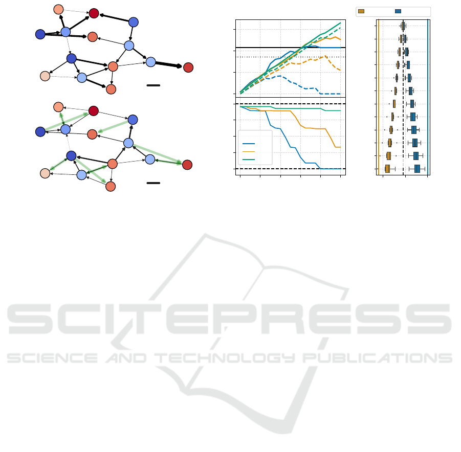
played in Fig. 1(a). The thickness and direction of

the lines indicate the physical power ﬂow obtained by

pandapower’s DC power ﬂow.

Fig. 1(b) shows the matches found by solving

the model exactly with Gurobi using parameters ρ =

45ct/kWh and α = 100ct/kWh

. The thickness of

the power lines indicates the mismatch between the

physical and logical power ﬂow here.

4.1 Collected Grid Operation Fees

In a non-P2P environment, electricity prices for cus-

tomers do not directly reﬂect production costs. Be-

sides taxes, a signiﬁcant portion is attributed to oper-

ational costs for maintaining and stabilizing the power

grid. In P2P markets, those costs still need to be

covered as the market members use the existing in-

frastructure and incur maintenance costs. Let us as-

sume that 50% of the purchase price for electricity is

the grid operation compound, i.e., 15 ct/kWh of the

30ct/kWh baseline

. The horizontal line in Fig. 1(c)

represents the total collected grid operation fees of the

DSO in the case14 non-P2P scenario.

The dashed lines in Fig. 1(c) indicate the total cost

allocation for different α’s depending on the grid fee

parameter ρ. As expected, the earnings from P2P

trades for the DSO increase with increasing ρ; how-

ever, they start to fall off again as soon as costs be-

come too expensive for the customers and they rather

trade directly with the DSO again. This is also vi-

sualized in Fig. 1(d), where the ratio of P2P trades

compared to total demand is shown. When customer

demand is not satisﬁed by P2P trades, it will be sat-

urated by direct DSO electricity purchases, enabling

the DSO to subsequently collect additional grid oper-

ation fees even if no P2P trades are facilitated. The

total collected grid operation fees are observable in

the solid-line plot in panel (c). For α = 10ct/kWh

we see that when no P2P trades occur, we precisely

retrieve the collected baseline operation fees.

Furthermore, it is apparent that the total retrieved

grid operation fees exhibit a similar trend up until they

are saturated (ρ < 60ct/kWh), independent of α. We,

therefore, require ρ ≈ 45ct/kWh to gain about 80%

of the baseline costs. The authors arbitrarily choose

Producers are not charged for grid operation in this as-

sumption.

Grid Cost Allocation in Peer-to-Peer Electricity Markets: Benchmarking Classical and Quantum Optimization Approaches

755

p10

c11

c12

p13

(a)

1 kWh

p10

c11

c12

p13

(b)

0.2 kWh

100

150

Grid Operation Costs [ct]

Baseline Operation Costs

80%

(c)

0 20 40 60 80 100

Grid Fee Parameter ρ [ct/kWh]

0.00

0.25

0.50

0.75

1.00

Ratio of demand

satisﬁed by P2P trades

(d)

α [ct/kWh

]

100

10 20 30

Eﬀective Tariﬀ [ct/kWh]

Grid Fee Parameter ρ [ct/kWh]

8ct/kWh sell

30ct/kWh buy

(e)

Producer Consumer

Figure 1: P2P power ﬂow matching on an example instance of the IEEE case14. Panel (a) shows the input data to the

optimization problem consisting of the net topology, the consumer and producer data, as well as the physical power ﬂow.

Below, in (b), we depict the solution to the optimization problem Eq. (10); the green arrows indicate the matched pairs and the

thickness of the power lines corresponds to the mismatch between physical and logical power ﬂow. In the center, (c) and (d),

the solution in terms of gathered grid operation costs is shown depending on the model parameters ρ and α. Finally, (e)

visualizes the effective tariffs in dependence of ρ for the consumers and producers separately.

80%, which is sensible since the self-balancing com-

munity, in which P2P trades are facilitated, causes

less strain on the power grid and, therefore, less oper-

ational costs.

4.2 Individual Customer Tariffs

Due to the different line usage, each customer will re-

ceive a different effective tariff composed of grid op-

eration cost allocation and the compensation between

consumer and producer. The ﬁnal price or tariff is

computed with Eqs. (11) and (12). Fig. 1 (e) shows

the different effective customer tariffs for consumers

and producers for different grid fee parameters ρ.

Clearly, at ρ = 0, all trades are free of charge. Hence,

the consumer and producer tariffs align at the equi-

librium tariff λ

= 19 ct/kWh. As the fee increases,

consumption becomes more expensive and produc-

tion less proﬁtable. The average consumption tariff

approaches the baseline tariff of λ

buy

= 30 ct/kWh,

while the consumer compensation tariff decreases to

sell

= 8ct/kWh. The experiments for the effective

customer tariffs shown here have been conducted with

α = 100ct/kWh

5 BENCHMARKS

One aim of this study is to evaluate the applicability of

quantum approaches to solving this problem. There-

fore, we compare the performance of different solvers

against each other in the following.

5.1 Experimental Setup

First, we explain the benchmarking setup, i.e., the

considered problem instances, solvers, and metrics.

5.1.1 Problem Instance Dataset

For testing on close-to real-world problems, we re-

quire grid topologies that resemble the future elec-

tricity grid, i.e., energy grids containing decentralized

power generation. To this end, we modify the IEEE

system test cases, as described in Sec. 4. For our anal-

ysis, we select the available IEEE test cases between

9 and 57 nodes, referred to in the following as case{9,

14, 24, 33, 39, 57} where the numbers denote the

number of nodes in the respective IEEE power sys-

tems test case. For each test case, we generate 20 in-

stances using different seeds to sample from the con-

sumption distributions to generate different load pro-

ﬁles.

Like Sec. 4, we determine ρ for each test case,

such that the DSO receives roughly 80% of the base-

line costs. Unsurprisingly, the grid topology signif-

icantly impacts the collected fees through cost allo-

cation. Therefore, we must set case-speciﬁc grid fee

constants, as seen in Table 1.

QAIO 2025 - Workshop on Quantum Artiﬁcial Intelligence and Optimization 2025

756

Table 1: ρ values and timeout settings for each case.

case 9 14 24 33 39 57

ρ[ct/kWh] 20 45 40 15 15 15

Timeout [s] 1 2.45 7.2 13.6 19 40.6

5.1.2 Investigated Solvers

We analyze the performance of classical branch-and-

cut (Gurobi), classical heuristics (SA, TS), hybrid

quantum-classical (Leap), and QA (D-Wave).

Speciﬁcally, we utilize D-Wave Advantage 5.4,

located in Germany. Since the embedding of the

fully connected optimization QUBO (10) onto the D-

Wave hardware graph is limited to maximally 169 bi-

nary variables, case33 with 272 binary variables is

already too large for D-Wave. For embedding, we

use the Clique embedder, a fast (polynomial-time) al-

gorithm designed explicitly for fully connected prob-

lems (Boothby et al., 2016).

On the other hand, Gurobi can be faced with

two equivalent problem formulations that make a

difference in runtime and solution quality. As the

QUBO (10) has a mean-squared-error form, we uti-

lize CVXPY(Diamond and Boyd, 2016) to interface

Gurobi. CVXPY formulates the optimization problem

as follows

min

∑

i, j

∑

p,c

s.t. ζ

i, j

= w

i, j

−v

i, j

(x) ∀i, (13)

where ζ

i, j

is the residual power ﬂow per line.

This formulation allows Gurboi to ﬁnd better lower

bounds more efﬁciently, leading to a faster converg-

ing branch-and-cut procedure. The second alterna-

tive is to present Gurobi the expanded expression of

Eq. (10), which is referred to in the following as

Gurobi[ncvx].

Since the solution bit-string will only be sparsely

populated with ones, i.e., only a tiny fraction of all

possible trades will be satisﬁed, we initialize the SA

solver with all bits set to zero. This will make the

exploration stage easier at the beginning since SA re-

quires a few bitﬂips to arrive at a viable solution.

To ensure a fair comparison, we optimize the hy-

perparameters of the classical heuristics and the D-

Wave QA. The results can be found in Table 2, and

further details are presented in the Appendix.

All classical experiments were conducted on a

single core of an AMD Ryzen Threadripper PRO

5965WX.

5.1.3 Benchmarking Strategies

In the following, we devise two benchmarking strate-

gies to compare the solvers on solution quality and

runtime.

Solution Quality Within Time Limit. For this

strategy, we set a ﬁxed timeout for each test case and

investigate how close the solutions are to the optimal

solution. The reference solution x

∗

is obtained by run-

ning Gurobi for one hour for each instance using the

formulation created with CVXPY (Diamond and Boyd,

2016). The relative objective error can then be com-

puted using

ε(x) =

C(x) −C(x

∗

)

C(x

∗

)

, (14)

where C(x) is the cost function deﬁned in Eq. (10).

We choose a linearly growing timeout with the

number of involved binary variables to mitigate the

growing problem difﬁculty with increasing problem

size. We set the timeout for each use case according to

the number of possible trades, i.e., |P×C|, or approx-

imately (N/2)

, which is subsequently used. We arbi-

trarily set case9 to 1s, and scale the remaining cases

accordingly, see Table 1. Leap has a minimal conﬁg-

urable time limit of 3 s, which overrides our timeout

setting.

Time to Solution (TTS). As we are investigating

some nondeterministic heuristics with varying suc-

cess probability, it is sensible to inspect the expected

time each solver requires to reach a solution of ade-

quate quality. This evaluation considers solutions ac-

ceptable if they are within 5% of the optimal solution

computed using Gurobi (ε ≤ 5%). Furthermore, we

only run experiments until case33, as the optimal so-

lution has not been found with Gurobi for the larger

cases, possibly distorting the TTS. The error threshold

is chosen since some solvers struggle to ﬁnd the op-

timal solution, disallowing TTS calculation. We run

each solver on each instance until 50 samples have

been found that are within 5% of the optimal solution.

However, since this might take a very long time, we

ﬁxed an upper limit of 1000 s. To ensure the statistical

signiﬁcance of our results, we disregard the TTS if we

do not ﬁnd at least 10 samples within the timeout.

TTS is computed by estimating the expected run-

time based on the sample time t

and the expected

number of repetitions to sample one solution with

99% probability, based on the probability measured

from the samples p

(Steiger et al., 2015)

TTS(ε) = t



log(1 −0.99)

log(1 − p

)



. (15)

Since Leap only has the time limit as a con-

trollable parameter, we cannot directly evaluate TTS

here. Instead, we investigate how a growing time limit

improves solution quality.

Grid Cost Allocation in Peer-to-Peer Electricity Markets: Benchmarking Classical and Quantum Optimization Approaches

757

case9 case14 case24 case33 case39 case57

−3

−2

−1

rel. objective error ε

ε = 5%

Gurobi

Gurobi[ncvx]

D-Wave

Leap

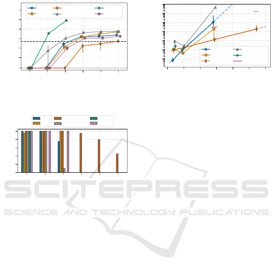
Figure 2: The median relative objective error for different

solvers and test cases. The error bars mark the 50% per-

centile interval. Gurobi’s median solution quality stays be-

low the 5% rel. error mark for almost all cases.

case9 case14 case24 case33 case39 case57

Solutions (ε ≤ 5%) found

Gurobi

Gurobi[ncvx]

D-Wave

Leap

Figure 3: Number of instances for which a solution within

the 5% error bound has been obtained.

5.2 Results

Solution Quality. Fig. 2 shows the relative er-

ror with the time limit from Table 1 for different

cases. We can see that, except for D-Wave and the

Gurobi[ncvx], almost all algorithms solve the ﬁrst

two cases to optimality. Afterward, we see a steep

decrease in solution quality for every solver, crossing

the 5% error threshold between case24 and case33

except for the convex Gurobi, which exhibits the low-

est error (< 5%). This is also highlighted in Fig. 3,

where Gurobi is the only algorithm that consistently

ﬁnds solutions that are within 5% of the optimal so-

lution for every case. SA, TS, and Leap perform sim-

ilarly, with Leap having a slight advantage. D-Wave

performs very poorly except for the smallest case (20

binary variables). It exhibits a mean relative error

of more than 20% in case14 and almost 1000% in

case24.

Notably, Gurobi[ncvx] performs considerably

worse than Gurobi and possesses higher solution

quality errors than the classical heuristics and the hy-

brid quantum algorithm.

0 50 100 150 200 250 300

Number of binary variables n

−3

−2

−1

TTS(5%) [s]

∝ 1.02

∝ 1.08

Gurobi

Gurobi[ncvx]

D-Wave

Leap

Figure 4: Median TTS to ﬁnd a solution that is within 5%

of the optimal solution with respect to the number of binary

variables in the optimization problem. Error bars indicate

the 50% percentile interval. D-Wave only shows a single

point since no solutions within the error bound were ob-

served for problem instances larger than case9.

Time to Solution. Fig. 4 presents the estimated

TTS results to reach solutions within the 5% error.

We are missing several data points because speciﬁc

solvers could not ﬁnd the minimum required amount

of acceptable samples within the timeout limit, as dis-

cussed in the following. Due to the solution quality

results, we did not attempt to ﬁnd TTS estimates with

D-Wave for cases larger than case9. Similarly, SA,

TS, Gurobi[ncvx] do not ﬁnd sufﬁcient satisfactory

solutions for case33, where they crossed the error 5%

error threshold in Fig. 2, even with the increased time

limit considered.

Both Gurobi and SA exhibit exponential runtime

scaling, as the linear dependence with the logarith-

mic time scale is distinctly visible. A linear regression

reveals exponential scaling with ∝ 1.08

for SA and

∝ 1.02

for Gurobi, with R

scores above 99%, where

n is the number of binary variables in the optimization

problem. Interestingly, TS and Gurobi[ncvx] both ex-

perience a similar dip in required runtime between

case9 and case14, indicating that case14 could be

easier than case9. However, this hypothesis is not

supported by the results from SA and Gurobi, indi-

cating a similarity between the solving strategy of

Gurobi[ncvx] and TS. Since the three data points of

TS and Gurobi[ncvx] do not exhibit apparent expo-

nential scaling, we do not perform linear regression

here. However, qualitatively, TS seems to scale simi-

larly to SA, and Gurobi[ncvx] scales worse than SA.

Focusing on the absolute TTS at the smallest

case9, we see that SA is fastest (< 1 ms), Gurobi and

TS come second with ≈ 10ms. Afterwards, we iden-

tify D-Wave (≈ 20 ms) and Gurobi[ncvx] (≈ 100ms)

as the slowest.

Since TTS analysis is impossible with D-Wave’s

Leap hybrid solver, we separately analyze the solution

QAIO 2025 - Workshop on Quantum Artiﬁcial Intelligence and Optimization 2025

758

Figure 5: D-Wave hybrid Leap BQM solver solution quality

improvement against timeout setting.

quality improvement upon growing time limit settings

in Fig. 5. Due to the minimum timeout of 3 s for

Leap, we cannot infer the TTS for case24 as it is cer-

tainly below 3 s. For case33, we can estimate that

the TTS is probably larger than 160 s, since the me-

dian point crosses the 5% threshold there. As a con-

sequence, the median TTS is about 160 s, which is

slower than Gurobi but probably faster than SA, judg-

ing from Fig. 4, where 3 s and 160 s are indicated with

faint pink horizontal lines.

5.3 Discussion

The results show that Gurobi—equipped with the

convex problem formulation—outperforms (or per-

forms on par with) every other solver in terms of so-

lution quality within a time limit. Only the TTS of

SA and TS is faster for the small test cases case9

and case14, as apparent from Fig. 4, which can be

explained by the fast sampling times of heuristics in

these small instances and initialization overhead of

the more complex Gurobi solver.

That Gurobi outperforms the classical and

quantum-classical heuristics is to some extent sur-

prising since the problem of Eq. (10) is inherently

of unconstrained form, which means no constraints

had to be formulated as penalty, which typically

makes problems more challenging to solve with un-

constrained solving algorithms (Lucas, 2014; Bucher

et al., 2024a). The analysis of both formulations for

Gurobi unmistakably showed that presenting Gurobi

with the convex formulation is advantageous. Our re-

sults on the scaling behavior of the TTS of Gurboi

and SA also show superior scaling of Gurobi com-

pared to SA, indicating that no break-even point can

be expected with growing problem size.

Furthermore, QA performs extremely sub-par in

this use case, already losing solution quality beyond

the accepted threshold of 5% relative error in the sec-

ond smallest test case. This result can be explained by

the embedding necessary to map the fully connected

problem structure onto the graph of the D-Wave hard-

ware. Even though we utilize the specialized Clique

embedding method for fully connected problems with

chain strength hyperparameter optimization, the em-

bedding still requires excessive amounts of physical

qubits for a single logical one.

Since the experimental results demonstrate that

classical heuristics and hybrid methods yield inferior

solutions compared to Gurobi, QA hardware advance-

ments may not help solve this problem more efﬁ-

ciently. Instead, we expect they merely close the gap

between the current quantum results and the classical

heuristics. We can make the same argument for other

heuristic quantum optimization algorithms, including

the gate-based Quantum Approximate Optimization

Algorithm (Farhi et al., 2014), challenging better ex-

perimental results than classical heuristics. However,

further experimental validation is necessary to con-

ﬁrm this hypothesis. Due to the large problem size

and deep quantum circuits required because of the

fully connected problem structure, this veriﬁcation is

currently out of reach for simulation or real hardware

experiments.

The ﬁndings from this speciﬁc problem of power

ﬂow matching tentatively suggest that binary least-

squares problems, or even binary convex problems,

might not be suitable candidates for quantum op-

timization applications, as they can be more efﬁ-

ciently solved using existing classical optimization

algorithms. However, more extensive studies are

needed to prove the generalization of this statement.

It is important to remark here that quantum special-

ized optimization methods for convex problems (Ab-

bas et al., 2024) have not been investigated within

that study but only QUBO optimization methods like

QA. Nevertheless, these oracle-based methods are ex-

pected only to apply when fault-tolerant QC is avail-

able.

6 CONCLUSION

This study had two objectives: ﬁrst, to develop an

optimization model for allocating grid usage costs in

P2P electricity markets, and second, to investigate

whether quantum optimization techniques can suc-

cessfully be employed to solve the deﬁned model.

For the ﬁrst part, we devised a binary optimization

model that aims to match the logical power ﬂow—the

power ﬂow that can be attributed to P2P consumer-

producer pairs—with the physical power ﬂow when

all producers and consumers in the network inject

(draw) power into (from) the grid. An in-depth in-

vestigation of the model behavior showed that this

Grid Cost Allocation in Peer-to-Peer Electricity Markets: Benchmarking Classical and Quantum Optimization Approaches

759

formulation could retrieve all collected grid operation

fees from beforehand. This indicates that the formula-

tion is viable for attributing P2P grid operation costs.

Nevertheless, the formulation is still rudimentary and

probably requires extensions (e.g., external grid con-

nection, baseline grid fees, and bidding constraints)

to make it applicable in a real-world scenario. Yet,

it serves as a sufﬁcient proof-of-concept use case for

benchmarking and a seed for future work.

The second goal is to show the applicability of

quantum optimization techniques. This is straightfor-

wardly possible as the problem formulation is already

in QUBO form, which is atypical in applied quantum

computing to real-world use cases. Thus, we directly

benchmarked QA against classical heuristics, hybrid

quantum-classical heuristics, and a classical branch-

and-cut solver. When posed with a convex formula-

tion of the least-squares problem, the classical solver

outperformed any heuristic, with QA performing sig-

niﬁcantly sub-par due to the fully connected nature of

the problem. This substantially challenges the valu-

able application of QA to solve the power ﬂow match-

ing problem, as classical methods ﬁnd better solutions

faster and exhibit more favorable scaling behavior.

Furthermore, these results indicate that binary

least-squares problems can be inherently challenging

for classical heuristics and quantum methods, unlike

linear least-squares results might suggest (Borle and

Lomonaco, 2018). Yet, this statement and whether

this consequence extends to general convex optimiza-

tion problems requires further experimental investi-

gation. Nevertheless, specialized convex quantum al-

gorithms such as Refs. (van Apeldoorn et al., 2020;

Chakrabarti et al., 2020; Abbas et al., 2024) may be

a more advanced future route for solving the power

ﬂow matching. Another route forward could be to in-

vestigate the spectral gap throughout the quantum an-

nealing process, which may give valuable insight into

whether the complete connectedness or the problem

itself is the main barrier to solving.

Finally, the authors suggest that future searches

for applications of quantum optimization algorithms

should focus on problems with sparser intercon-

nections and structures that are not classically ex-

ploitable, such as unconstrained and non-convex

problems.

ACKNOWLEDGEMENTS

The authors would like to thank Kumar Ghosh

and Naeimeh Mohsehni for their helpful discussions

throughout this research. This work was supported by

the German Federal Ministry of Education and Re-

search under the funding program “F

orderprogramm

Quantentechnologien – von den Grundlagen zum

Markt” (funding program quantum technologies —

from basic research to market), project Q-Grid,

13N16177.

REFERENCES

Abbas, A., Ambainis, A., Augustino, B., B

artschi, A., and

et al. (2024). Challenges and opportunities in quantum

optimization. Nature Reviews Physics, pages 1–18.

Baroche, T., Pinson, P., Latimier, R. L. G., and Ahmed,

H. B. (2019). Exogenous Cost Allocation in Peer-to-

Peer Electricity Markets. IEEE Transactions on Power

Systems, 34(4):2553–2564.

Blenninger, J., Bucher, D., Cortiana, G., Ghosh, K.,

Mohseni, N., N

ußlein, J., O’Meara, C., Porawski, D.,

and Wimmer, B. (2024). Q-GRID: Quantum Opti-

mization for the Future Energy Grid. KI - K

unstliche

Intelligenz.

Boothby, T., King, A. D., and Roy, A. (2016). Fast

clique minor generation in Chimera qubit connectivity

graphs. Quantum Information Processing, 15(1):495–

508.

Borle, A. and Lomonaco, S. J. (2018). Analyzing the Quan-

tum Annealing Approach for Solving Linear Least

Squares Problems.

Born, M. and Fock, V. (1928). Beweis des Adiabatensatzes.

Zeitschrift f

ur Physik, 51(3):165–180.

Bucher, D., Kraus, N., Blenninger, J., Lachner, M., Stein,

J., and Linnhoff-Popien, C. (2024a). Towards Robust

Benchmarking of Quantum Optimization Algorithms.

Bucher, D., Porawski, D., Wimmer, B., N

ußlein, J.,

O’Meara, C., Mohseni, N., Cortiana, G., and

Linnhoff-Popien, C. (2024b). Evaluating Quantum

Optimization for Dynamic Self-Reliant Community

Detection.

Chakrabarti, S., Childs, A. M., Li, T., and Wu, X. (2020).

Quantum algorithms and lower bounds for convex op-

timization. Quantum, 4:221.

Christie, R., Wollenberg, B., and Wangensteen, I. (2000).

Transmission management in the deregulated environ-

ment. Proceedings of the IEEE, 88(2):170–195.

Colucci, G., Linde, S. V. D., and Phillipson, F. (2023).

Power Network Optimization: A Quantum Approach.

IEEE Access, 11:98926–98938.

D-Wave (2020). Hybrid Solver System: An Overview.

https://www.dwavesys.com/resources/white-paper/d-

wave-hybrid-solver-service-an-overview/.

Diamond, S. and Boyd, S. (2016). CVXPY: A Python-

Embedded Modeling Language for Convex Optimiza-

tion. https://arxiv.org/abs/1603.00943v2.

Doan, H. T., Cho, J., and Kim, D. (2021). Peer-to-peer

energy trading in smart grid through blockchain: A

double auction-based game theoretic approach. IEEE

Access, 9:49206–49218.

Farhi, E., Goldstone, J., and Gutmann, S. (2014). A Quan-

tum Approximate Optimization Algorithm.

QAIO 2025 - Workshop on Quantum Artiﬁcial Intelligence and Optimization 2025

760

Farhi, E., Goldstone, J., Gutmann, S., Lapan, J., Lundgren,

A., and Preda, D. (2001). A Quantum Adiabatic Evo-

lution Algorithm Applied to Random Instances of an

NP-Complete Problem. Science, 292(5516):472–475.

Fern

andez-Campoamor, M., O’Meara, C., Cortiana, G.,

Peric, V., and Bernab

e-Moreno, J. (2021). Commu-

nity Detection in Electrical Grids Using Quantum An-

nealing.

Glover, F. (1989). Tabu Search—Part I. ORSA Journal on

Computing, 1(3):190–206.

Gurobi Optimization (2024). Gurobi Optimizer Reference

Manual.

Kea, K., Huot, C., and Han, Y. (2023). Leveraging Knap-

sack QAOA Approach for Optimal Electric Vehicle

Charging. IEEE Access, 11:109964–109973.

Kirkpatrick, S., Gelatt, C. D., and Vecchi, M. P. (1983).

Optimization by Simulated Annealing. Science,

220(4598):671–680.

Le Cadre, H., Jacquot, P., Wan, C., and Alasseur, C. (2020).

Peer-to-peer electricity market analysis: From vari-

ational to Generalized Nash Equilibrium. European

Journal of Operational Research, 282(2):753–771.

Lucas, A. (2014). Ising formulations of many NP problems.

Frontiers in Physics, 2.

Mastroianni, C., Plastina, F., Scarcello, L., Settino, J.,

and Vinci, A. (2024). Assessing Quantum Comput-

ing Performance for Energy Optimization in a Pro-

sumer Community. IEEE Transactions on Smart Grid,

15(1):444–456.

McGeoch, C. and Farr

e, P. (2021). The Advantage System:

Performance Update. Technical report.

Mohseni, N., Morstyn, T., Meara, C. O., Bucher, D.,

ußlein, J., and Cortiana, G. (2024). A Competitive

Showcase of Quantum versus Classical Algorithms in

Energy Coalition Formation.

Muhsen, H., Allahham, A., Al-Halhouli, A. T., Al-

Mahmodi, M., Alkhraibat, A., and Hamdan, M.

(2022). Business model of peer-to-peer energy trad-

ing: A review of literature. Sustainability.

Nielsen, M. A. and Chuang, I. L. (2010). Quantum Compu-

tation and Quantum Information. Cambridge univer-

sity press, Cambridge, 10th anniversary edition edi-

tion.

O’Meara, C., Fern

andez-Campoamor, M., Cortiana, G., and

Bernab

e-Moreno, J. (2023). Quantum Software Ar-

chitecture Blueprints for the Cloud: Overview and

Application to Peer-2-Peer Energy Trading. In 2023

IEEE Conference on Technologies for Sustainability

(SusTech), pages 191–198.

Rajak, A., Suzuki, S., Dutta, A., and Chakrabarti,

B. K. (2023). Quantum Annealing: An Overview.

Philosophical Transactions of the Royal Society A:

Mathematical, Physical and Engineering Sciences,

381(2241):20210417.

Rønnow, T. F., Wang, Z., Job, J., Boixo, S., Isakov, S. V.,

Wecker, D., Martinis, J. M., Lidar, D. A., and Troyer,

M. (2014). Deﬁning and detecting quantum speedup.

Science, 345(6195):420–424.

Sousa, T., Soares, T., Pinson, P., Moret, F., Baroche, T., and

Sorin, E. (2019). Peer-to-peer and community-based

markets: A comprehensive review. Renewable and

Sustainable Energy Reviews, 104:367–378.

Steiger, D. S., Rønnow, T. F., and Troyer, M. (2015). Heavy

Tails in the Distribution of Time to Solution for Classi-

cal and Quantum Annealing. Physical Review Letters,

115(23):230501.

Thurner, L., Scheidler, A., Sch

afer, F., Menke, J.-H., Dol-

lichon, J., Meier, F., Meinecke, S., and Braun, M.

(2018). Pandapower—An Open-Source Python Tool

for Convenient Modeling, Analysis, and Optimization

of Electric Power Systems. IEEE Transactions on

Power Systems, 33(6):6510–6521.

van Apeldoorn, J., Gily

en, A., Gribling, S., and de Wolf, R.

(2020). Convex optimization using quantum oracles.

Quantum, 4:220.

APPENDIX

Table 2: Optimal hyperparameters for D-Wave.

case

9 14 24

chain strength factor 0.3 0.4 0.9

annealing time [µs] 10 20 20

To ensure fair benchmark comparison, we aim to de-

vote equal effort to hyperparameter optimization of

the individual solvers (Bucher et al., 2024a). Leap

cannot be ﬁne-tuned, and Gurobi, as a commercial

solver, is also considered with default parameters.

Preliminary experiments showed little to no response

of TS to changing hyperparameters; hence, we do not

consider it in the following section. Instead, we only

consider SA and D-Wave in the following, whose re-

sults are summarized in Table 2.

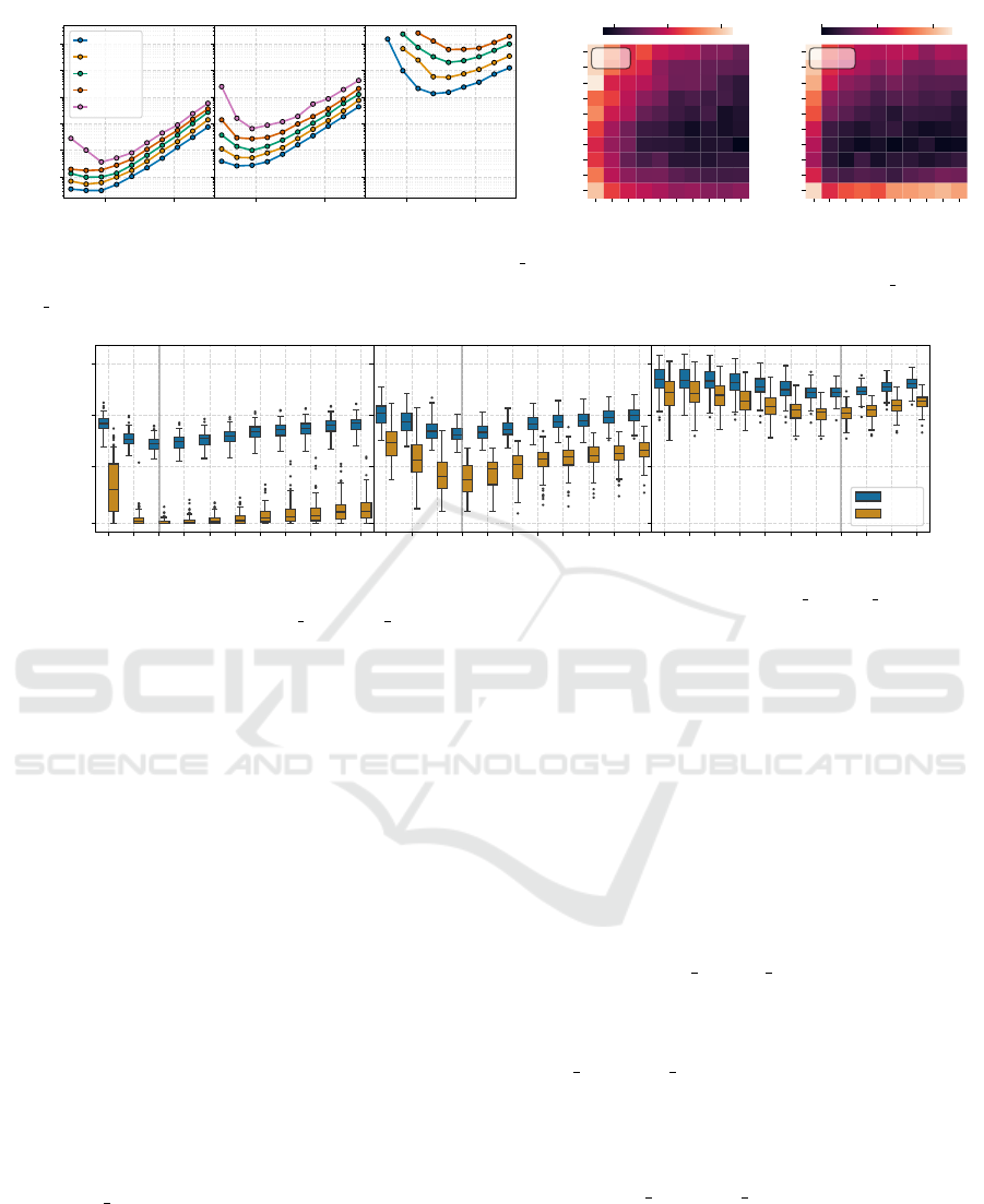
Simulated Annealing

The most critical hyperparameter of SA is the num-

ber of Monte Carlo sweeps (num sweeps) computed

for a single sample. A larger number of sweeps re-

sults in better solutions, but the runtime for a single

sample of the algorithm is directly proportional to the

number of sweeps in the algorithm. Therefore, we

expect a TTS sweet spot when tuning num sweeps,

similar to Refs. (Rønnow et al., 2014; Steiger et al.,

2015). Indeed, Fig. 6 shows that the smaller instances

exhibit an optimal TTS of around 100 sweeps, while

case24 is optimal with around 1000 sweeps. For the

larger test cases, it was not really possible to estimate

the TTS correctly, as the samples were consistently

above the 5% error threshold. Hence, we heuristically

set increasing num sweeps for these instances: 5000

sweeps for case33 and case39 and 10000 for case57.

The second set of parameters investigated is the

Grid Cost Allocation in Peer-to-Peer Electricity Markets: Benchmarking Classical and Quantum Optimization Approaches

761

num_sweeps

−3

−2

−1

TTS(5%) [s]

case9

q = 25%

q = 50%

q = 75%

q = 90%

q = 99%

num_sweeps

case14

num_sweeps

case24

beta_end

0.001

0.005

0.02

0.1

beta_start

case9

0.0010 0.0015 0.0020

beta_end

0.001

0.005

0.02

0.1

case14

0.01 0.02 0.03

Figure 6: Left-hand side shows the TTS of SA for different num sweeps with annealing schedule (0.02, 1000) showcasing

different quantiles. The two heatmaps on the right show the 75% quantile TTS depending on different beta start and

beta end parameters of the annealing schedule for case9 and case14 at 100 Monte Carlo sweeps.

0.1 0.2 0.3 0.4 0.5 0.6 0.8 0.9 1.0 1.2 1.4

chain_strength_factor

rel. objective error ε

case9

0.1 0.2 0.3 0.4 0.5 0.6 0.8 0.9 1.0 1.2 1.4

chain_strength_factor

case14

0.1 0.2 0.3 0.4 0.5 0.6 0.8 0.9 1.0 1.2 1.4

chain_strength_factor

case24

mean

min

Figure 7: Average and Minimum relative energy error of D-Wave Advantage 5.4 with different chain strength factors. Gray

vertical lines mark the optimal chain strength factor.

start- and end-point of the geometric annealing sched-

ule of SA. Since we have a ﬁxed starting point, where

all bits are set to zero, we conjecture that the opti-

mal annealing schedule stays similar throughout dif-

ferent problem sizes. The right two plots of Fig. 6

show combinations of different start and end values

as a heatmap of case9 and case14. Visually, we ob-

serve a similar large region with good TTS values

for both cases, centered around (0.2,1000). Since

the high computational demand required for this par-

ticular investigation, we only conducted it on case9

and case14. Nevertheless, we tested the (0.2, 1000)

parameter setting against the default (automatically

calculated) schedule for all instances and ultimately

received better results averaged over all instances.

Hence, we argue that this setting is overall beneﬁcial,

even if it may not be the best one for a single instance.

D-Wave

The most prominent parameter for QA is the

annealing time, governing the overall time of the

annealing process. In theory, a longer annealing time

should result in better solution quality. However, due

to the error-prone NISQ hardware, longer times most

often introduce too much error, resulting in unusable

samples. Nevertheless, our experiments showed lit-

tle to no effect of the annealing time on the solution

quality. Only a slight indication was found that for

case9 10 µs is optimal, while for the remaining cases,

the default 20 µs worked best.

As explained in the main text, embedding the fully

connected QUBO problem onto the D-Wave QPU

hardware graph requires the aggregation of multi-

ple physical qubits to a single logical qubit to repli-

cate the connectedness required for the input prob-

lem. Technically, this is done by augmenting the op-

timization problem with large biases between qubits

belonging to the same binary variable. The strength

of this interaction is commonly calculated using

D-Wave’s uniform torque compensation. How-

ever, it is heuristically computed from the biases in

the input problem, so the strength setting may not

be optimal. Therefore, we scale the bias using a

chain strength factor that weakens the interac-

tions if less than 1 and strengthens them otherwise.

Fig. 7 shows the minimum and mean relative en-

ergy error from 1000 samples. We can observe a min-

imum in all three embeddable cases, indicating the

optimal chain strength factor (Table 2).

Finally, we also conducted initial experiments on

annealing schedule parameters (including reverse an-

nealing) but abolished that route due to insigniﬁcant

effects on the result.

QAIO 2025 - Workshop on Quantum Artiﬁcial Intelligence and Optimization 2025

762