Quantum-Efﬁcient Kernel Target Alignment

Rodrigo Coelho

, Georg Kruse

1,2

and Andreas Rosskopf

Fraunhofer IISB, Erlangen, Germany

Technical University Munich, Germany

{rodrigo.coelho, georg.kruse, andreas.rosskopf}@iisb.fraunhofer.de

Keywords:

Quantum Machine Learning, Quantum Kernels, Kernel Target Alignment.

Abstract:

In recent years, quantum computers have emerged as promising candidates for implementing kernels. Quan-

tum Embedding Kernels embed data points into quantum states and calculate their inner product in a high-

dimensional Hilbert Space by computing the overlap between the resulting quantum states. Variational Quan-

tum Circuits (VQCs) are typically used for this end, with Kernel Target Alignment (KTA) as cost function. The

optimized kernels can then be deployed in Support Vector Machines (SVMs) for classiﬁcation tasks. However,

both classical and quantum SVMs scale poorly with increasing dataset sizes. This issue is exacerbated in quan-

tum kernel methods, as each inner product requires a quantum circuit execution. In this paper, we investigate

KTA-trained quantum embedding kernels and employ a low-rank matrix approximation, the Nystr

om method,

to reduce the quantum circuit executions needed to construct the Kernel Matrix. We empirically evaluate the

performance of our approach across various datasets, focusing on the accuracy of the resulting SVM and the

reduction in quantum circuit executions. Additionally, we examine and compare the robustness of our model

under different noise types, particularly coherent and depolarizing noise.

1 INTRODUCTION

Quantum computers may potentially solve certain

problems faster than classical computers. However,

in the Noisy Intermediate Scale Quantum (NISQ) era,

we are limited in the algorithms that quantum com-

puters can implement (Preskill, 2018). Consequently,

algorithms that theoretically offer advantages over the

best-known classical methods, such as Shor’s (Shor,

1999) and Grover’s (Grover, 1996) algorithms, cannot

yet be implemented to tackle problems of industrial

signiﬁcance. In the NISQ era, quantum computing

has focused on Variational Quantum Circuits (VQCs).

These circuits rely on free parameters that are iter-

atively updated by a classical optimizer. VQCs are

suitable for NISQ devices due to their low require-

ments in both number of qubits and circuit depth,

which mitigates noise effects (Cerezo et al., 2021).

Typically used as function approximators, VQCs are

the quantum analog of Neural Networks (NNs), as

both are black-box models that depend on parame-

ters iteratively adjusted to minimize a cost function

(Abbas et al., 2021). Given their potential, VQCs

have been extensively applied in machine learning

and form a signiﬁcant component of Quantum Ma-

chine Learning (QML). Notable examples include

the Quantum Approximate Optimization Algorithm

(QAOA) (Farhi et al., 2014) for solving combinato-

rial optimization problems, the Variational Quantum

Eigensolver (VQE) (Kandala et al., 2017) for ﬁnding

ground states of Hamiltonians, and their application

in both supervised (Schuld, 2018) and reinforcement

(Skolik et al., 2022) learning.

On the classical side, kernel methods are one of

the cornerstones of machine learning, known for their

effectiveness in handling non-linear data by using im-

plicit feature spaces. These methods map input data

into a higher-dimensional space where linear separa-

tion is possible, facilitated by the kernel trick, which

computes inner products in this space without explic-

itly performing the transformation. Support Vector

Machines (SVMs) are a prime example, leveraging

kernel methods to ﬁnd optimal decision boundaries

for classiﬁcation tasks (Hearst et al., 1998). Even

though we’ll focus on SVMs throughout this work,

kernel methods can be applied to many tasks beyond

classiﬁcation, ranging from regression (Drucker et al.,

1996) to clustering (Dhillon et al., 2004).

In recent years, interest in exploring how quan-

tum computing can enhance kernel methods has in-

creased. Quantum computers, can naturally pro-

cess high-dimensional spaces, providing a promising

Coelho, R., Kruse, G. and Rosskopf, A.

Quantum-Efﬁcient Kernel Target Alignment.

DOI: 10.5220/0013391500003890

Paper published under CC license (CC BY-NC-ND 4.0)

In Proceedings of the 17th International Conference on Agents and Artiﬁcial Intelligence (ICAART 2025) - Volume 1, pages 763-772

ISBN: 978-989-758-737-5; ISSN: 2184-433X

763

platform for implementing kernels. For this reason,

they have been extensively explored recently (Wang

et al., 2021)(J

ager and Krems, 2023).We are inter-

ested in Quantum Embedding Kernels (QKEs), which

use quantum circuits to embed data points into a

high-dimensional Hilbert space. The overlap between

these quantum states is then used to compute the in-

ner product between data points in this feature space.

Typically, these kernels are parameterized, making

them a form of VQCs. The parameters of these cir-

cuits are optimized based on Kernel Target Alignment

(KTA), which serves as a metric to align the kernel

with the target task (which we will consider to be bi-

nary classiﬁcation) (Hubregtsen et al., 2022). Once

the kernel is optimized, it is fed into an SVM to de-

termine the optimal decision boundary for the classi-

ﬁcation task at hand. This integration leverages the

strengths of both quantum and classical computing,

aiming to enhance classiﬁcation performance due to

the expressive power of quantum embeddings com-

bined with the robust framework of SVMs.

However, the method scales poorly. For instance,

using the KTA as cost function requires calculat-

ing the kernel matrix at every single training step, a

process that scales quadratically O(N

) with train-

ing dataset size N. To alleviate this, both the origi-

nal paper (Hubregtsen et al., 2022) and a following

one (Sahin et al., 2024) propose using only a subsam-

ple of size D ≪ N of the training dataset to compute

the KTA at each epoch, effectively turning the com-

putation, which becomes O(D

), independent of N.

Moreover, another paper (Tscharke et al., 2024) pro-

poses using a clustering algorithm to ﬁnd centroids

of the classes and then computing the kernel matrix

with respect to these centroids at each training step,

bringing the complexity of the computation to O(N).

So, these methods are able to decrease the complex-

ity of training from scaling quadratically with N to

either scaling only linearly or even being completely

independent of N. Nonetheless, the end goal is for

the optimized kernel matrix, which contains the pair-

wise inner-products between all training data points,

to be fed into the SVM. Thus, at least for this ﬁnal

computation, these methods still require O(N

) com-

putations. This is especially important if we consider

that each pairwise inner-product requires a quantum

circuit execution.

In this paper, we adapt a low-rank matrix approx-

imation known as the Nystr

om Approximation, which

is commonly used in classical kernel methods, to ad-

dress this scalability issue. This approach reduces

the complexity of computing the kernel matrix from

O(N

) to O(NM

), where M ≪ N is an hyperparam-

eter that determines the quality of the approximation.

The Nystr

om Approximation is applied for comput-

ing the optimized kernel matrix that is fed into the

SVM, resulting in a classiﬁcation pipeline that scales

linearly with the training dataset size N in all steps.

Consequently, our method facilitates the efﬁcient ap-

plication of quantum kernel methods to industrially-

relevant problems.

The contributions of this paper are organized as

follows:

• Adapted the Nystr

om Approximation to Quantum

Embedding Kernels

• Empirically veriﬁed (on several synthetic

datasets) that, in a noiseless setting, the Nystr

Approximation method allows for quantum

kernels with reduced quantum circuit executions

at a small cost in the accuracy of the resulting

SVM.

• Empirically tested the performance of the devel-

oped method under both coherent and incoherent

noise.

2 KERNEL METHODS AND

SUPPORT VECTOR MACHINES

Kernel methods can be used for different tasks, from

dimensionality reduction (Sch

olkopf et al., 1997) to

regression (Drucker et al., 1996). We will focus on bi-

nary classiﬁcation using SVMs, which are linear clas-

siﬁers (Hearst et al., 1998). Nonetheless, they can be

used in non-linear classiﬁcation problems due to the

kernel trick, which implicitly maps the data into high-

dimensional feature spaces where linear classiﬁcation

is possible. In this section we will go through this

pipeline for classiﬁcation, starting with kernel meth-

ods and ending with SVMs.

2.1 Kernel Methods

Consider a dataset X = {(x

, y

)}

i=1

, where x

∈ R

with d being the number of features of x

. A kernel

method involves deﬁning a feature map φ : R

→ H ,

where H is a high-dimensional Hilbert space. The

kernel function can then be deﬁned as:

k(x

, x

) = ⟨φ(x

), φ(x

)⟩

(1)

Put in words, the kernel function computes the

inner product between the inputs x

and x

in some

high-dimensional feature space H . Given the kernel

function k, the kernel matrix K is a symmetric matrix

that contains the pairwise evaluations of k over all the

points in the training dataset X:

QAIO 2025 - Workshop on Quantum Artiﬁcial Intelligence and Optimization 2025

764

i j

= K(x

, x

) = ⟨φ(x

), φ(x

)⟩

(2)

Typically, explicitly calculating the coordinates of

the input points in the high-dimensional feature space,

a task that may be computationally expensive, is not

needed. Instead, the kernel trick allows one to efﬁ-

ciently compute these inner products without needing

to explicitly calculate the feature map φ.

For example, consider the Radial Basis Function

(RBF) kernel, deﬁned as:

RBF

(x, y) = exp



−γ∥x − y∥



(3)

where γ is an hyperparameter that the user deﬁnes.

This kernel computes the inner product between the

data points x and y in an inﬁnite-dimensional feature

space given by the feature map ϕ

RBF

. However, due to

the kernel trick, one only needs to compute the kernel

RBF

and not the feature map ϕ

RBF

, saving computa-

tional resources.

2.2 Support Vector Machines

An SVM aims to ﬁnd the optimal hyperplane that sep-

arates data points of two different classes with the

maximum margin. This margin is the distance be-

tween the hyperplane and the nearest data points from

either class, known as support vectors (Hearst et al.,

1998). SVMs are inherently linear classiﬁers; they

work effectively when the dataset is linearly separa-

ble by a hyperplane.

However, the kernel trick extends SVMs to non-

linear datasets. By using a kernel function, the data

is implicitly mapped into a high-dimensional feature

space where linear separation is feasible. Thus, with

the aid of the kernel trick, SVMs can classify non-

linear datasets.

Given a kernel matrix K containing the pairwise

inner-products between all training points x ∈ X, the

optimization problem the SVM solves is formulated

as:

min

∑

i=1

∑

j=1

K(x

, x

) −

∑

i=1

(4)

where α

are the Lagrange multipliers. An SVM

solves a quadratic problem and thus is guaranteed to

converge to the global minimum.

The decision function is given by:

f (x) = sign

∑

i=1

K(x

, x) + b

(5)

Here, b is the bias term, often determined using

the support vectors. However, as shown in Equation

4, training an SVM on a dataset of size N requires

Figure 1: One layer of the quantum ansatz used through-

out this work. As an example, this layer in particular con-

tains 4 qubits. The ansatz contains input scaling parameters

λ and variational parameters θ. The data encoding gates

(blue-colored) are repeated in every single layer - data re-

uploading.

computing N

pairwise inner products to construct the

kernel matrix K. This implies that the runtime scales

at least quadratically with the training dataset size N.

Moreover, even after obtaining the kernel matrix K,

the SVM must solve a quadratic optimization prob-

lem. Depending on the data structure and the algo-

rithm used, this process may scale with N

or even N

Consequently, SVMs are typically applied to small-

scale problems with moderate dataset sizes.

3 QUANTUM EMBEDDING

KERNELS

The ﬁrst step to solve a classical problem using a

quantum computer is to encode the classical data into

a quantum state that can be processed by quantum op-

erations. Given a data point x, one can deﬁne a quan-

tum circuit U(x) to generate said quantum state:

ϕ(x)

⟩

= U(x)

⟩

(6)

This corresponds to embedding the data in a high-

dimensional Hilbert space. Referring back to Equa-

tion 1, a kernel function is deﬁned as the inner prod-

uct between two data points in a high-dimensional

Hilbert space. In the context of quantum computing,

this translates to calculating the ﬁdelity between the

quantum states generated by encoding the two data

points. The ﬁdelity, which measures the similarity be-

tween these quantum states, is given by:

k(x

, x

) =



⟨ϕ(x

)|ϕ(x

)⟩



(7)

There are several ways to calculate the ﬁdelity be-

tween two quantum states. In particular, assuming

that ϕ(x) and ϕ(y) are pure quantum states (that is,

Trace(ρ

) = 1, where ρ =

⟨

⟩

), then the ﬁdelity can

be calculated using the adjoint of the quantum circuit

(Hubregtsen et al., 2022):

K(x, y) =

⟨ϕ(x)|ϕ(y)⟩



⟨0|U

†

(y)U(x)|0⟩



(8)

Quantum-Efﬁcient Kernel Target Alignment

765

(a) . (b) .

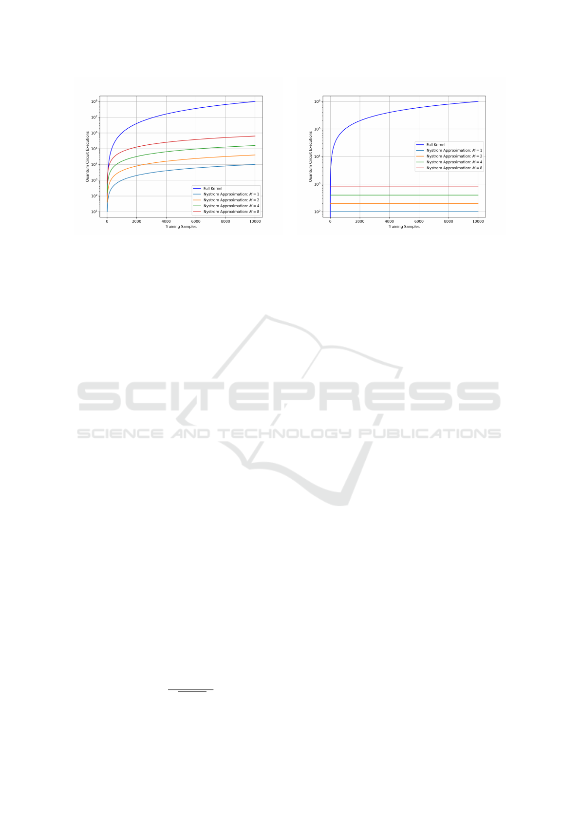
Figure 2: Quantum circuit executions required for computing the training kernel matrix (Fig.2a) and testing kernel matrix

(Fig.2b) as a function of the training dataset size N for the standard approach and the Nystr

om approximation with different

Ms.

This is equivalent to the probability of observing

⟩

when measuring U

(y)U(x)

⟩

in the computa-

tional basis.

We have established a deﬁnition for quantum ker-

nels. Nevertheless, the choice of which quantum ker-

nel to use remains unclear. In Noisy-Intermediate

Scale Quantum (NISQ) devices, a popular approach

is to make the circuit trainable, deﬁne a cost function,

and optimize the parameters using a classical opti-

mizer. These methods are known as Variational Quan-

tum Algorithms. In our speciﬁc case, a quantum ker-

nel can be made trainable by making the quantum cir-

cuit U (x) also depend on these classical parameters,

becoming U(x, θ). Thus, the kernel function from Eq.

8 becomes:

(x, y) =



⟨0|U

†

(y,θ)U(x, θ)|0⟩



(9)

Then, the question becomes what cost function to

use. Following paper (Hubregtsen et al., 2022), we

use Kernel-Target Alignment (KTA) as our cost func-

tion, which predicts the alignment between the quan-

tum kernel K

and the labels of the training data. We

start by deﬁning an ideal kernel using the labels of the

training data:

, x

) = y

(10)

Then, assuming y ∈ {−1, 1}, k

will be 1 if both

labels belong to the same class and −1 otherwise.

This ideal kernel matrix can be deﬁned as:

= y

y (11)

Then, the KTA can be deﬁned as:

KTA =

Tr(K

(12)

In this context, N represents the total number of

training samples in the dataset. Since we want to min-

imize a cost function and maximize KTA, we will in-

clude a negative sign in this equation during training.

4 NYSTR

OM APPROXIMATION

To reduce the complexity of computing the ker-

nel matrix, one can use the Nystr

om approxima-

tion (Drineas et al., 2005). It works as follows.

The ﬁrst step is to select a subset of M ≪ N data

points from the original training dataset N, referred

to as landmarks. In this work, we will always

select the landmarks randomly, but they can also

be selected according to more sophisticated strate-

gies, such as K-means clustering. Then, compute

the matrix K

of shape (M, M) using the selected

subset where, given landmarks {m

, m

, ..., m

(i, j) = ⟨φ(m

), φ(m

)⟩

. Then, compute the

cross-kernel matrix K

of shape (N, M) between the

M landmarks and the N training data points. Finally,

the Nystr

om approximation of the kernel matrix K is

given by:

K ≈ K

−1

(13)

If we disregard the computational cost of invert-

ing K

(as this step is performed classically), the

Nystr

om approximation reduces the computational

cost of calculating the kernel matrix from O(N

) to

O(NM

). Consequently, the number of quantum cir-

cuit executions required to compute the matrix now

scales linearly with N, signiﬁcantly enhancing efﬁ-

ciency in the quantum context.

This method can also be used to reduce the com-

putational cost of generating the kernel matrix to clas-

QAIO 2025 - Workshop on Quantum Artiﬁcial Intelligence and Optimization 2025

766

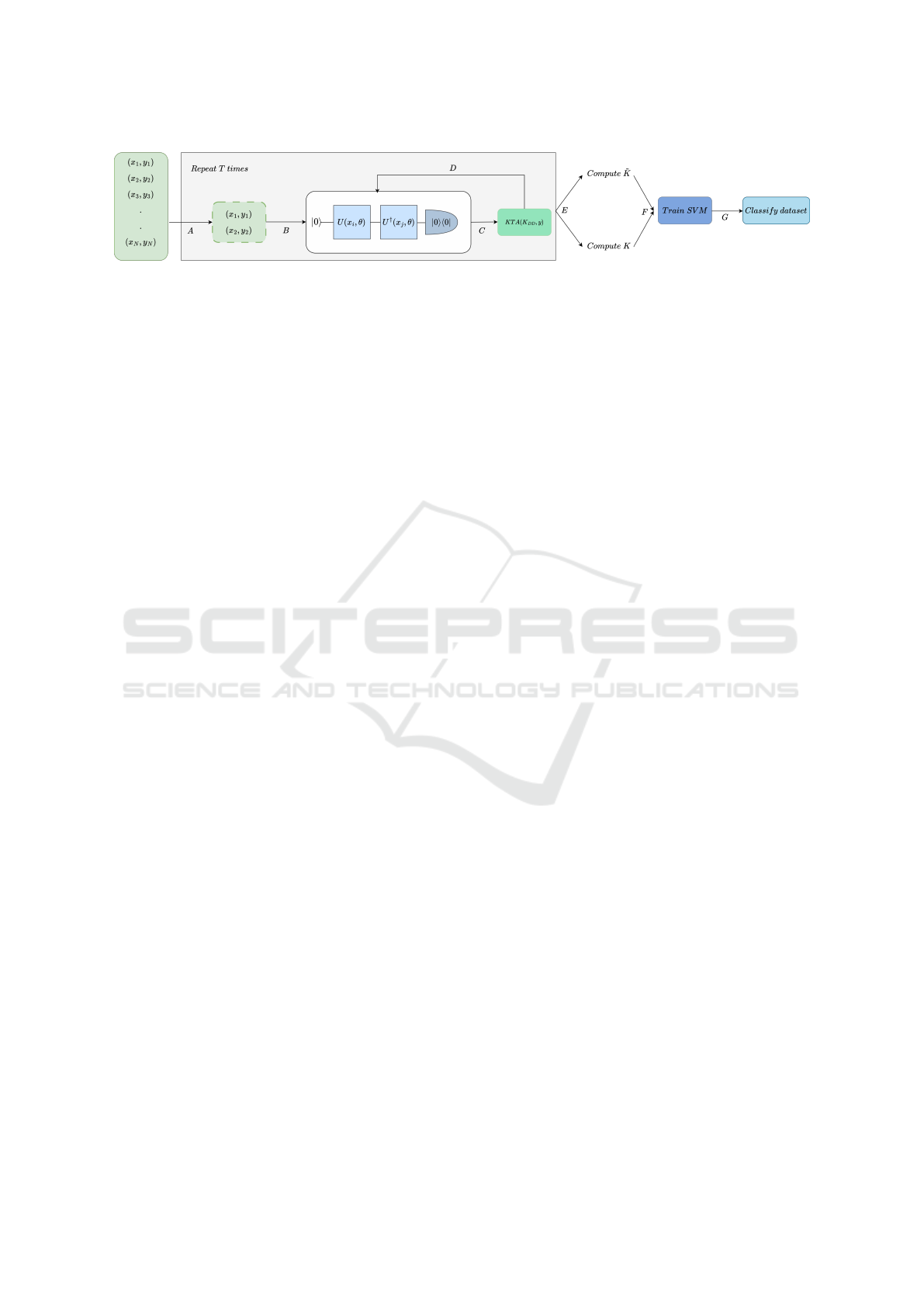
Figure 3: Given a training dataset of size N, for T iterations, do: A) sample a random mini-batch of data points of size D. B)

Calculate the overlap between the embedded quantum states. C) Once all the pairs have been processed, ﬁll the kernel matrix

and compute the cost function (KTA). D) Update the parameters θ of the quantum circuit. Finally, after the T training

iterations, E) Compute the approximated training kernel matrix

K using either the Nystr

om approximation method or the full

training kernel matrix K using the standard approach. F) Use the training kernel matrix to ﬁt an SVM to the dataset and G)

Classify the training dataset.

sify a test dataset. The end goal in classiﬁcation tasks

is to test the model on unseen data points. With an

SVM, this requires generating a testing kernel ma-

trix of shape (P, N), where P is the size of the test-

ing dataset, leading to a computational complexity of

O(PN). However, using the Nystr

om approximation,

one can reduce this computational cost to O(PM),

making it independent of the training dataset size N.

This is accomplished by computing:

test

≈ K

−1

(14)

Here, K

is the cross-kernel matrix between the

M landmarks and the P test data points, and K

the previously computed cross-kernel matrix between

the M landmarks and the N training data points. For

a comparison in terms of the number of quantum cir-

cuit executions required to construct the training and

testing kernel matrices using either the Nystr

om ap-

proximation or the standard approach, see Fig.2

5 METHOD

In this work, we test the Nystr

om approximation

method for generating the kernel matrix that is fed

into the SVM in the context of quantum embedding

kernels. We start with a training dataset with N data

points and an ansatz for the VQC, see Fig. 1, ran-

domly initializing the free parameters. The quantum

circuit is then trained over T training iterations using

the KTA as the cost function.

However, calculating the kernel matrix K for ev-

ery training iteration is computationally expensive.

To mitigate this, we adopt a strategy similar to that

used in (Hubregtsen et al., 2022; Sahin et al., 2024).

At each iteration, we randomly sample a mini-batch

of D training points, construct their kernel matrix

, calculate the KTA for this mini-kernel, and up-

date the parameters using a classical optimizer. Con-

sequently, the number of quantum circuit executions

per training iteration becomes independent of the size

of the training dataset N and instead scales quadrati-

cally with D. Since, as we will see, D can be chosen

such that D ≪ N, this method signiﬁcantly reduces

the number of quantum circuit executions required

per training iteration.

After completing the T training iterations and op-

timizing the quantum kernel for the task at hand,

we compute the kernel matrix for the entire training

dataset N using the Nystr

om approximation method.

This is our main contribution in this work. Using this

approximation allows us to build the kernel matrix

that is fed into the SVM at the end of training using

only O(NM

) (where M is the number of landmarks),

quantum circuit executions, instead of the O(N

) exe-

cutions that both (Hubregtsen et al., 2022) and (Sahin

et al., 2024) require. To our knowledge, this is the ﬁrst

pipeline in which the number of quantum circuit ex-

ecutions scales linearly with the training dataset size

N in all steps. Speciﬁcally, the training process has a

complexity of O(D

), and the computation of the ﬁnal

kernel matrix of O(NM

) (note that this complexity

takes into account only the number of quantum cir-

cuit executions). The entire pipeline can be seen in

Fig.3.

Although not explicitly shown in the ﬁgure, the

Nystr

om approximation method saves quantum cir-

cuit executions in comparison with the standard ap-

proach during inference as well, when classifying a

testing dataset. The standard approach has a (quan-

tum) complexity of O(NP), with P being the size of

the testing dataset, while the Nystr

om approximation

has a complexity of O(PM).

Lastly, we wish to explain in higher depth the dif-

ferences between the method from (Sahin et al., 2024)

and the Nystr

om approximation method we propose

here. In short, they are different methods with dif-

ferent applications. The method from (Sahin et al.,

2024) allows us to use KTA as the cost function with-

out computing a full kernel matrix at each training

step. Instead, it computes a mini-kernel matrix K

reducing quantum circuit executions from O(N

) to

Quantum-Efﬁcient Kernel Target Alignment

767

(a) . (b) .

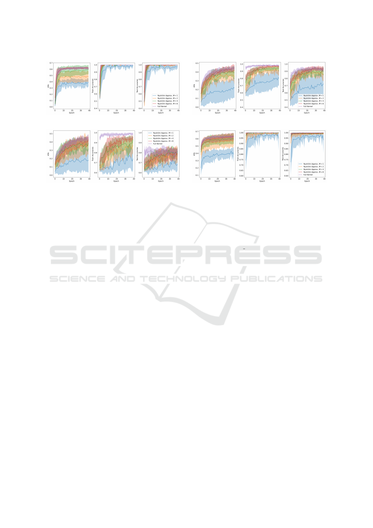
Figure 4: Performance of the Standard approach VS the Nystr

om approximation with different Ms throughout training mea-

sured through KTA, training and testing accuracy in the checkers (Fig. 4a), corners (Fig. 4b), donuts (Fig. 4c) and spirals

(Fig. 4d) datasets.

O(D

), where D ≪ N. This is essentially a type of

stochastic gradient descent, where KTA is approxi-

mated by using a subset of data points.

After training, the SVM requires the full opti-

mized kernel matrix to classify the training dataset.

Therefore, we cannot use the previous method here,

as the SVM needs the complete matrix (O(N

) quan-

tum circuit executions) rather than a mini-version

based on a subsample. The Nystr

om Approximation

method addresses this need by computing an approxi-

mated full-kernel matrix

K while reducing the number

of quantum circuit executions to O(NM

). Thus, us-

ing both methods —(Sahin et al., 2024) during train-

ing and the Nystr

om Approximation for generating

the kernel matrices once training is done —results in

a pipeline that scales linearly with the training dataset

size in all steps.

We can also apply the Nystr

om Approximation

during the T training iterations instead of the method

from (Sahin et al., 2024) by using the approximated

kernel matrix

K to compute KTA. However, this does

not reduce quantum circuit executions and, based on

limited experiments, did not yield signiﬁcantly better

results. Therefore, in this work, we use the method

from (Sahin et al., 2024) during training.

6 NUMERICAL RESULTS

In this section, we empirically compare the Nystr

approximation method and the standard method on

a set of simple binary 2D classiﬁcation tasks. The

datasets selected include the checkers and donuts

datasets from (Hubregtsen et al., 2022), a manually

created corners dataset, and the spirals dataset gener-

ated using the make moons method from scikit-learn.

For a more detailed explanation, please refer to Ap-

pendix 8.

To compare the methods, we will use three met-

rics: the KTA between the current quantum kernel

and the ideal kernel for the entire training dataset, the

training accuracy, and the testing accuracy. Note that

calculating the ﬁrst two metrics requires computing

the training kernel matrix, while the last metric re-

quires computing the testing kernel matrix. This is

where the standard approach and the Nystr

om approx-

imation differ, as previously explained. Due to the in-

herent randomness of parameter initialization, results

are averaged over 10 seeds and plotted alongside the

standard deviation.

For the experiments, the input scaling weights are

initialized as 1s, ensuring they initially have no effect

on the output of the quantum kernel, and the varia-

tional weights sampled uniformly between −π and π.

The methods were implemented using PyTorch and

PennyLane and all results obtained using state-vector

simulators. The parameters were optimized using the

ADAM optimizer with a learning rate of 0.1 and the

ansatz had a constant depth of 5 layers. Moreover,

during the training iterations, we always used a mini-

batch size D = 8.

QAIO 2025 - Workshop on Quantum Artiﬁcial Intelligence and Optimization 2025

768

(a) .

(b) .

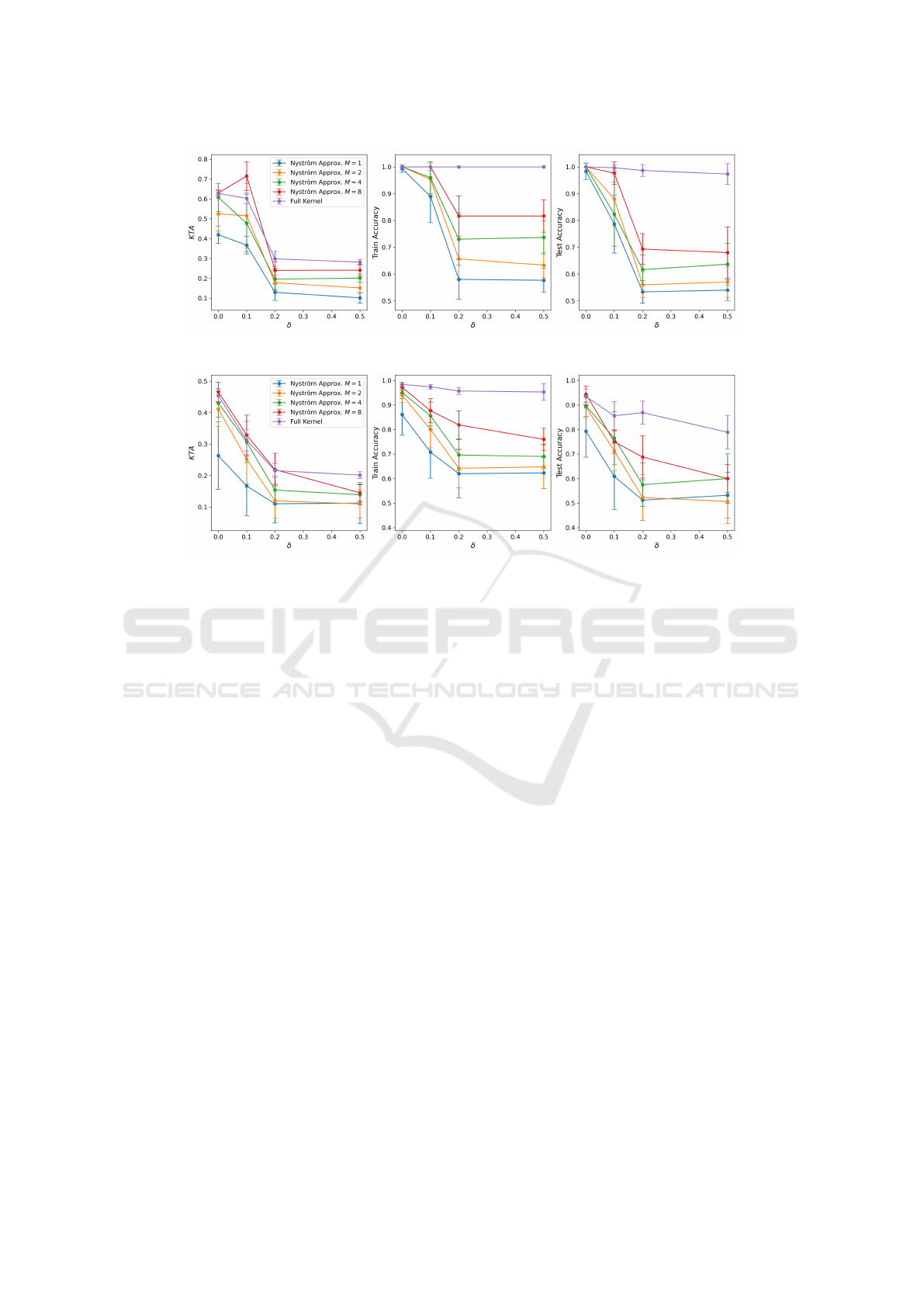
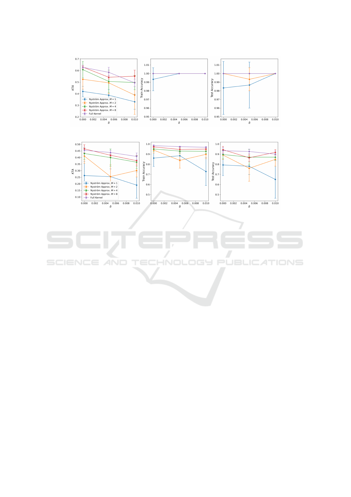
Figure 5: Performance of the Standard approach VS the Nystr

om approximation with different Ms for an increasing strength

of coherent noise σ in the checkers (Fig.5a) and corners dataset (Fig.5b).

6.1 Method Comparison on Noiseless

Simulator

We will start by analyzing both methods in ideal con-

ditions, that is, in the absence of noise.

The performance comparison between the stan-

dard approach and the Nystr

om approximation on

four benchmark datasets is illustrated in Fig.4.

As observed in the KTA graphs, the standard ap-

proach consistently achieves the highest KTA across

all four datasets. Moreover, a lower value of M typ-

ically results in a reduced KTA for the Nystr

om ap-

proximation method. This is expected, as lower val-

ues of M lead to less accurate approximations of the

training and testing kernel matrices. However, this

lower KTA does not necessarily imply reduced accu-

racies, as evidenced by the training and testing results.

In some datasets, the Nystr

om method achieves both

training and testing accuracies of 100%, despite the

lower KTA.

These ﬁndings suggest an important considera-

tion: if one is willing to potentially sacriﬁce a slight

amount of accuracy for a signiﬁcantly reduced num-

ber of quantum circuit executions, the Nystr

om Ap-

proximation should be considered. Moreover, it’s also

clear that the training approach from (Sahin et al.,

2024) of using a mini-batch of size D every train-

ing step works, since in all datasets both accuracy and

KTA increased throughout training.

However, some nuances should be discussed. It’s

not clear precisely how both M and D are related to

the datasets’ complexity and/or size. We used sev-

eral training datasets with sizes ranging from 30 to

100 training data points and observed that, for all of

them, D = 8 and M ∈ {2, 4, 8} lead to considerably

high accuracies, achieving near or perfect classiﬁca-

tion on most of the datasets. However, for larger

and more complex datasets, it may be necessary to

increase both the values of D and M. It may also

be helpful to select the D data points and M land-

marks not randomly but instead based on more so-

phisticated techniques. For instance, the M landmarks

for the Nystr

om approximation technique can be se-

lected using k-means clustering, ensuring that they

are representative of the entire dataset, effectively bet-

ter approximating the kernel matrix. However, test-

ing such techniques is out of the scope of this work,

which intends to simply demonstrate for the ﬁrst time

a quantum-kernel pipeline that depends only linearly

on the training dataset size. In short, we do not claim

that the values of M and D used in this work and the

technique we used to select them (uniformly random

sampling) are guaranteed to provide good results for

any dataset. In fact, this pipeline should be highly

Quantum-Efﬁcient Kernel Target Alignment

769

dependent upon the dataset and, consequently, these

hyperparameters should be carefully chosen.

These results are in ideal conditions, if one had

access to a perfect quantum computer. In the next

subsections we will look at how the methods compare

under different types of noise.

6.2 Method Comparison Under

Coherent Noise

Coherent noise are errors that preserve the unitary

evolution of the quantum circuit but that still affect its

output (Cai et al., 2020). In (Skolik et al., 2023), co-

herent noise was modeled as under or over-rotations

of the parametrized quantum gates, which can be seen

as a miscalibration of the quantum gates. We will fol-

low a similar approach. The variational quantum pa-

rameters θ will be changed according to θ → θ + δθ,

where δθ are sampled according to a Gaussian distri-

bution of mean 0 and variance σ

. The perturbations

δθ are re-sampled if a new observable is being mea-

sured or if the circuit is being evaluated with a differ-

ent set of parameters (Skolik et al., 2023).

The performance of both the standard approach

and the Nystr

om approximation under increasing

strength of coherent noise σ can be seen in Fig. 5.

Firstly, it is evident that the standard approach

demonstrates better resistance to coherent noise. For

both datasets, although the KTA decreases signiﬁ-

cantly as σ increases, the training and testing accu-

racy only slightly decline for the corners dataset. In

contrast, the Nystr

om approximation method shows

a sharp decrease in KTA, training, and testing ac-

curacy when σ > 0.2. Furthermore, as observed in

the noiseless setting, lower values of M tend to per-

form worse. These results are unsurprising, as the

Nystr

om method approximates the kernel matrix us-

ing only a limited number of quantum circuit execu-

tions. If these executions are noisy, it is expected that

the resulting approximation will be even less accu-

rate. In summary, the approximation and the noise

compound, whereas the standard approach can toler-

ate more noise.

6.3 Method Comparison Under

Depolarizing Noise

In this section, we aim to analyze the performance

of both methods under a different type of noise: De-

polarizing Noise. This noise affects a quantum state

by replacing it with a mixed state with probability p,

or leaving it unchanged otherwise. It’s important to

highlight that, in the presence of device noise, the ad-

joint operation required to compute the quantum ker-

nel function may not be feasible. However, as shown

in (Hubregtsen et al., 2022), it is indeed possible in

the case of depolarizing noise.

In Pennylane, depolarizing noise can be imple-

mented using the Depolarizing Channel operation.

We model this type of noise by introducing single-

qubit depolarizing channels after each quantum gate.

The performance of both methods under depolar-

izing noise as a function of the probability p can be

seen in Fig.6.

Here too, similar results can be observed. The

standard approach is more robust against depolariz-

ing noise when compared with the Nystr

om method.

Nonetheless, both methods are able to effectively

reach high training and testing accuracies. In particu-

lar, if one uses the Nystr

om method with a larger M,

then the results are at least comparable to the stan-

dard approach, while still requiring substantially less

quantum circuit executions.

7 CONCLUSION

In this work we adapted a low-rank matrix approx-

imation method named Nystr

om approximation to

quantum embedding kernels, effectively reducing the

number of quantum circuit executions required to

construct the training and testing kernel matrices. In

doing so, we also introduce the ﬁrst quantum ker-

nel pipeline that has an end-to-end quantum complex-

ity that depends only linearly on the training dataset

size N. Other works had already introduced a linear

complexity during the training stage, but not during

the training matrix creation. Furthermore, we show

that, in the noiseless scenario, an SVM trained from a

quantum kernel using the Nystr

om approximation has

a performance comparable to that of an SVM trained

using the standard quantum kernel approach, without

any approximation. Finally, we compare both meth-

ods in the presence of coherent and depolarizing noise

and empirically demonstrate that both methods per-

form well under realistic levels of noise.

CODE AVAILABILITY

The source code for replicating the results is available

on Github at https://github.com/RodrigoCoelho7/

qekta.

QAIO 2025 - Workshop on Quantum Artiﬁcial Intelligence and Optimization 2025

770

(a) .

(b) .

Figure 6: Performance of the Standard approach VS the Nystr

om approximation with different Ms for an increasing proba-

bility of depolarizing noise p in the checkers (Fig.6a) and corners dataset (Fig.6b).

ACKNOWLEDGEMENTS

The research is part of the Munich Quantum Valley,

which is supported by the Bavarian state government

with funds from the Hightech Agenda Bayern Plus.

REFERENCES

Abbas, A., Sutter, D., Zoufal, C., Lucchi, A., Figalli, A.,

and Woerner, S. (2021). The power of quantum neural

networks. Nature Computational Science, 1(6):403–

409.

Cai, Z., Xu, X., and Benjamin, S. C. (2020). Mitigating

coherent noise using pauli conjugation. npj Quantum

Information, 6(1):17.

Cerezo, M., Arrasmith, A., Babbush, R., Benjamin, S. C.,

Endo, S., Fujii, K., McClean, J. R., Mitarai, K., Yuan,

X., Cincio, L., et al. (2021). Variational quantum al-

gorithms. Nature Reviews Physics, 3(9):625–644.

Dhillon, I. S., Guan, Y., and Kulis, B. (2004). Kernel k-

means: spectral clustering and normalized cuts. In

Proceedings of the tenth ACM SIGKDD international

conference on Knowledge discovery and data mining,

pages 551–556.

Drineas, P., Mahoney, M. W., and Cristianini, N. (2005). On

the nystr

om method for approximating a gram matrix

for improved kernel-based learning. journal of ma-

chine learning research, 6(12).

Drucker, H., Burges, C. J., Kaufman, L., Smola, A., and

Vapnik, V. (1996). Support vector regression ma-

chines. Advances in neural information processing

systems, 9.

Farhi, E., Goldstone, J., and Gutmann, S. (2014). A

quantum approximate optimization algorithm. arXiv

preprint arXiv:1411.4028.

Grover, L. K. (1996). A fast quantum mechanical algorithm

for database search. In Proceedings of the twenty-

eighth annual ACM symposium on Theory of comput-

ing, pages 212–219.

Hearst, M. A., Dumais, S. T., Osuna, E., Platt, J., and

Scholkopf, B. (1998). Support vector machines. IEEE

Intelligent Systems and their applications, 13(4):18–

28.

Hubregtsen, T., Wierichs, D., Gil-Fuster, E., Derks, P.-J. H.,

Faehrmann, P. K., and Meyer, J. J. (2022). Train-

ing quantum embedding kernels on near-term quan-

tum computers. Physical Review A, 106(4):042431.

ager, J. and Krems, R. V. (2023). Universal expressive-

ness of variational quantum classiﬁers and quantum

kernels for support vector machines. Nature Commu-

nications, 14(1):576.

Kandala, A., Mezzacapo, A., Temme, K., Takita, M.,

Brink, M., Chow, J. M., and Gambetta, J. M. (2017).

Hardware-efﬁcient variational quantum eigensolver

Quantum-Efﬁcient Kernel Target Alignment

771

for small molecules and quantum magnets. nature,

549(7671):242–246.

Preskill, J. (2018). Quantum computing in the nisq era and

beyond. Quantum, 2:79.

Sahin, M. E., Symons, B. C., Pati, P., Minhas, F., Mil-

lar, D., Gabrani, M., Mensa, S., and Robertus, J. L.

(2024). Efﬁcient parameter optimisation for quantum

kernel alignment: A sub-sampling approach in varia-

tional training. Quantum, 8:1502.

Sch

olkopf, B., Smola, A., and M

uller, K.-R. (1997). Kernel

principal component analysis. In International con-

ference on artiﬁcial neural networks, pages 583–588.

Springer.

Schuld, M. (2018). Supervised learning with quantum com-

puters. Springer.

Shor, P. W. (1999). Polynomial-time algorithms for prime

factorization and discrete logarithms on a quantum

computer. SIAM review, 41(2):303–332.

Skolik, A., Jerbi, S., and Dunjko, V. (2022). Quantum

agents in the gym: a variational quantum algorithm

for deep q-learning. Quantum, 6:720.

Skolik, A., Mangini, S., B

ack, T., Macchiavello, C., and

Dunjko, V. (2023). Robustness of quantum reinforce-

ment learning under hardware errors. EPJ Quantum

Technology, 10(1):1–43.

Tscharke, K., Issel, S., and Debus, P. (2024). Quack:

Quantum aligned centroid kernel. arXiv preprint

arXiv:2405.00304.

Wang, X., Du, Y., Luo, Y., and Tao, D. (2021). Towards un-

derstanding the power of quantum kernels in the nisq

era. Quantum, 5:531.

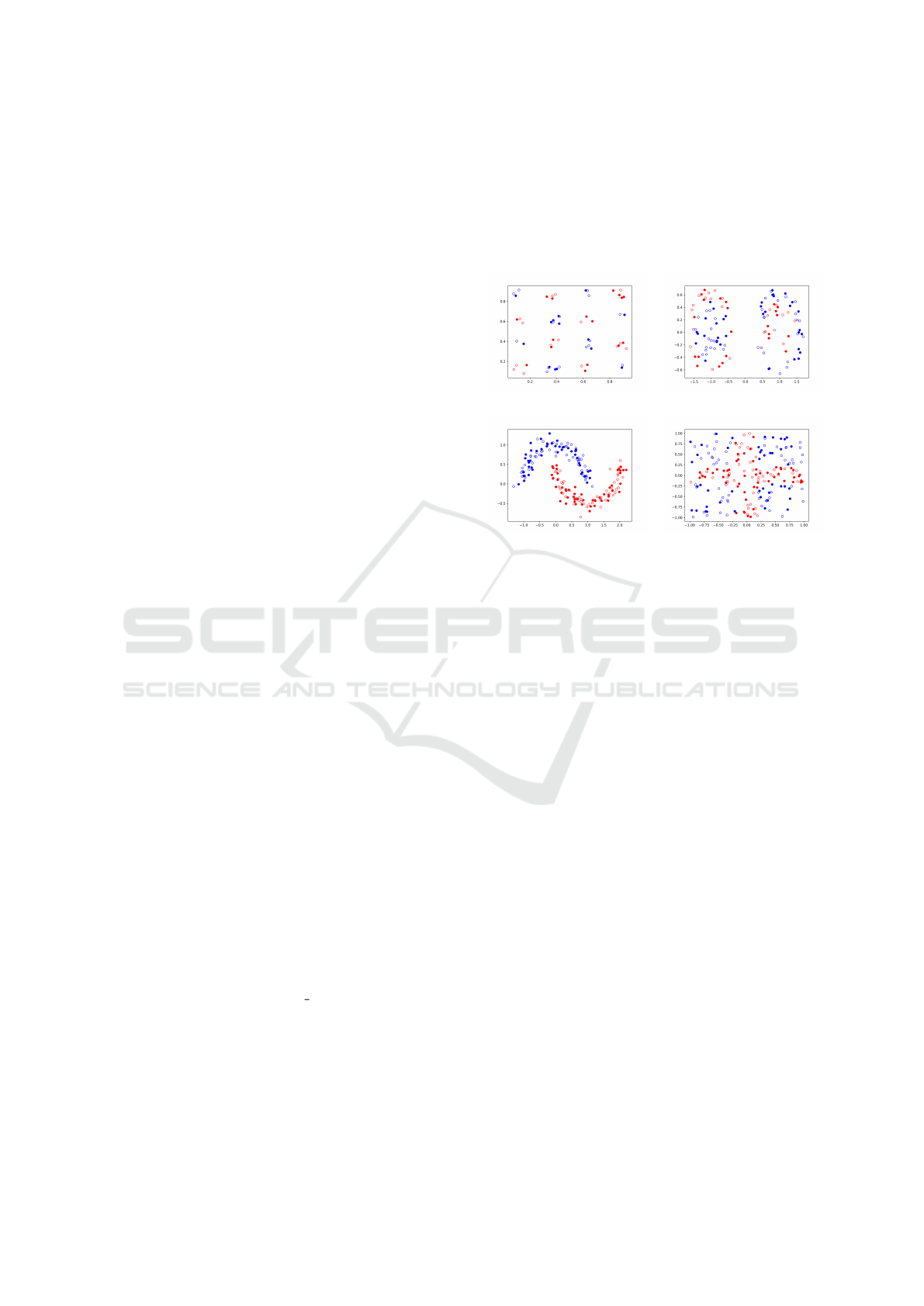
APPENDIX

The four binary 2D datasets used in this work for

benchmarking the models can be seen on Fig.7. A

speciﬁcation of the datasets and how to create them:

• Checker from (Hubregtsen et al., 2022). This

dataset consists of 30 training and 30 testing data

points. Used on both noiseless and noisy numeri-

cal results. The reader is referred to (Hubregtsen

et al., 2022) for more details on how to create it.

• Donuts from (Hubregtsen et al., 2022). This

dataset consists of 60 training and 60 testing data

points. Used on noiseless numerical results. The

reader is referred to (Hubregtsen et al., 2022) for

more details on how to create it.

• Spirals from scipy’s make moons method. This

dataset consists of 100 training and 100 testing

data points. Used on noiseless numerical results.

• Corners. This dataset consists of 100 training and

100 testing data points. To generate the dataset,

we ﬁrst deﬁne a square of size 2 (both x and y-

axis are between −1 and 1) and randomly sample

a set of points within this region. Each point is

then classiﬁed based on its location relative to four

quarter circles, each centered at one of the corners

of the square. Speciﬁcally, if a point falls within

any of these quarter circles, it is labeled as −1;

otherwise, it is labeled as 1. Used on noiseless

and noisy

(a) Checkers Dataset. (b) Donuts Dataset.

Figure 7: Red and blue represent the two classes. Cir-

cles/Circumferences represent training/testing data points.

QAIO 2025 - Workshop on Quantum Artiﬁcial Intelligence and Optimization 2025

772