Benchmarking Quantum Reinforcement Learning
Georg Kruse
1,2
, Rodrigo Coelho
1
, Andreas Rosskopf
1
, Robert Wille
2
and Jeanette-Miriam Lorenz
3,4
1
Fraunhofer IISB, Erlangen, Germany
2
Technical University Munich, Germany
3
Ludwig Maximilian University, Germany
4
Fraunhofer IKS, Munich, Germany
Keywords:
Quantum Reinforcement Learning, Quantum Boltzmann Machines, Parameterized Quantum Circuits.
Abstract:
Quantum Reinforcement Learning (QRL) has emerged as a promising research field, leveraging the principles
of quantum mechanics to enhance the performance of reinforcement learning (RL) algorithms. However,
despite its growing interest, QRL still faces significant challenges. It is still uncertain if QRL can show any
advantage over classical RL beyond artificial problem formulations. Additionally, it is not yet clear which
streams of QRL research show the greatest potential. The lack of a unified benchmark and the need to evaluate
the reliance on quantum principles of QRL approaches are pressing questions. This work aims to address these
challenges by providing a comprehensive comparison of three major QRL classes: Parameterized Quantum
Circuit based QRL (PQC-QRL) (with one policy gradient (QPG) and one Q-Learning (QDQN) algorithm),
Free Energy based QRL (FE-QRL), and Amplitude Amplification based QRL (AA-QRL). We introduce a
set of metrics to evaluate the QRL algorithms on the widely applicable benchmark of gridworld games. Our
results provide a detailed analysis of the strengths and weaknesses of the QRL classes, shedding light on the
role of quantum principles in QRL and paving the way for future research in this field.
1 INTRODUCTION
Quantum Reinforcement Learning (QRL) has gained
significant attention in recent years. Various ap-
proaches have been proposed to leverage the prin-
ciples of quantum mechanics to enhance the perfor-
mance of classical reinforcement learning (RL) algo-
rithms. Initially, QRL research focused on amplitude
amplification techniques applied to tasks like grid-
world navigation (Dong et al., 2008). The emergence
of quantum annealers like D-Wave led to the devel-
opment of free energy based learning using Quan-
tum Boltzmann Machines (QBMs) (Crawford et al.,
2018). Most recently, the widespread use of param-
eterized quantum circuits (PQC), often referred to as
quantum neural networks (Abbas et al., 2021), has led
to a wider range of applications of QRL algorithms.
Despite its growing interest, QRL still faces sig-
nificant challenges. While it is still uncertain whether
QRL can outperform classical RL, it is also unclear
which QRL approach holds the most promise. Un-
til now, only a limited number of works (e.g. (Neu-
mann et al., 2023)) have compared the various classes
of QRL algorithms against each other and no uni-
fied benchmarks have been proposed. A critical gap
in QRL research is the lack of studies examining
whether any performance enhancements are due to
quantum properties: (Bowles et al., 2024) have raised
questions about the reliance of quantum models on
entanglement and superposition. This work seeks
to contribute to this discourse by examining whether
QRL algorithms genuinely rely on their quantum
parts, or if algorithms without them can achieve sim-
ilar results.
Hence, we provide a comprehensive comparison
of three of the most widely spread QRL classes:
Parameterized Quantum Circuit based QRL (PQC-
QRL) (with one policy gradient (QPG) and one Q-
Learning (QDQN) algorithm), Free Energy based
QRL (FE-QRL), and Amplitude Amplification based
QRL (AA-QRL), which we will briefly introduce in
Section 2. We compare these QRL approaches us-
ing a series of metrics, including the number of re-
quired quantum circuit executions and the estimated
quantum clock time. In addition to these metrics we
will also investigate whether or not the performance
relies on the quantum properties of the quantum ap-
proaches.
Kruse, G., Coelho, R., Rosskopf, A., Wille, R. and Lorenz, J.-M.
Benchmarking Quantum Reinforcement Learning.
DOI: 10.5220/0013393200003890
Paper published under CC license (CC BY-NC-ND 4.0)
In Proceedings of the 17th International Conference on Agents and Artificial Intelligence (ICAART 2025) - Volume 1, pages 773-782
ISBN: 978-989-758-737-5; ISSN: 2184-433X
Proceedings Copyright © 2025 by SCITEPRESS – Science and Technology Publications, Lda.
773

By establishing a benchmark which is applicable
to various QRL algorithms, this paper aims to serve
as a resource for future QRL research to facilitate a
clearer understanding of the relative merits and chal-
lenges of each quantum approach. Through a detailed
analysis of performance metrics and quantum proper-
ties, we aim to guide the development of novel QRL
algorithms.
2 PRELIMINARIES
At their core, all RL algorithms, whether classical or
quantum, share a common structure centered around
the interaction between an agent and its environment.
The agent, responsible for making decisions, consists
of a function approximator that learns through inter-
actions with its environment - the external surround-
ings that influence and respond to the agent’s actions.
The agent’s ultimate goal is to develop a strategy that
maximizes the reward it receives from the environ-
ment.
Most RL environments are modeled as Markov
Decision Processes (MDPs). An MDP is character-
ized by its state space S, its action space A, a state
transition probability function P, denoting the prob-
ability of transitioning at time step t from state s
t
to
the next state s
t+1
after taking action a
t
, and a reward
function R, which quantifies the immediate value of
each state-action combination. This reward mecha-
nism serves as the learning signal, guiding the agent
towards optimal behavior through the maximization
of cumulative rewards.
In the field of QRL, various classes of algorithms
have been proposed. While covering all classes is be-
yond the scope of this work, we will focus on the
most established ones that can be applied to the most
generic benchmark case, namely gridworld games
(we will motivate the choice of gridworld games in
Section 3.1). We refer the reader to a comprehensive
overview of the field of QRL to the review by (Meyer
et al., 2022). In this work, we will focus on three
classes of QRL, which we will briefly introduce in
the following subsections.
2.1 Parameterized Quantum Circuit
Based QRL
In Deep Reinforcement Learning (DRL), deep neural
networks (DNNs) serve as powerful function approx-
imators. In the stream of research which we will refer
to as PQC-QRL, the DNNs are replaced with PQCs.
This approach has gained significant attention among
researchers due to its simplicity and natural similarity
to classical RL methods, leading to numerous imple-
mentations with varying circuit designs (Coelho et al.,
2024) (Kruse et al., 2024). However, the influence
of the chosen ansatz remains poorly understood, em-
phasizing the critical need for systematic benchmark-
ing efforts. Current research often builds upon the
hardware-efficient ansatz (HEA), which has been ini-
tially used by (Chen et al., 2020) and (Jerbi et al.,
2021a) and later improved upon, notably by (Skolik
et al., 2022) with data re-uploading and trainable out-
put scaling parameters.
encoding block
variational block
entangling block
|0⟩
|0⟩
|0⟩
RX(s
1
λ
1
) RZ(θ
1
) RY (θ
4
)
RX(s
2
λ
2
) RZ(θ
2
) RY (θ
5
)
RX(s
3
λ
3
) RZ(θ
3
) RY (θ
6
)
Figure 1: A single-layer PQC U
θ,λ
(s) for PQC-QRL is typ-
ically composed of three blocks that are repeated in each
layer: an encoding block, where the features of the state
(potentially scaled by trainable parameters λ) are encoded;
a variational block, with parameterized quantum gates; and
an entangling block. However, this structure is flexible, al-
lowing the blocks to be rearranged, combined, or modified
as needed. In this work we utilize the depicted ansatz as
proposed by (Skolik et al., 2022).
The evaluation of various ansatz design choices
would be beyond the scope of this work and has also
been conducted in previous works by (Dr
˘
agan et al.,
2022) and (Kruse et al., 2023). Instead, our evalu-
ation aims to establish a benchmark across various
algorithmic approaches that future studies can build
upon and progressively enhance. Hence, in this work,
we use the ansatz proposed by (Skolik et al., 2022).
Similarly to classical RL, quantum implementations
commonly utilize Policy Gradient (PG), Q-Learning
(in the form of DQNs), and actor-critic approaches
like Proximal Policy Optimization (PPO) as training
algorithms. Our investigation focuses on analyzing
the performance of quantum implementations of PG
and DQN which we will refer to as QPG and QDQN,
respectively.
2.1.1 Q-Learning
Q-Learning is a value-based algorithm that estimates
the expected return or value of taking a particular
action in a given state. The Q-function is defined
by mapping a tuple (π, s,a) of a given policy π, a
current state s, and an action a to the expected value
of the current and future discounted rewards. This is
formally expressed through the action-value function
QAIO 2025 - Workshop on Quantum Artificial Intelligence and Optimization 2025
774

Q
π
(s
t
,a
t
) = E
π
[G
t
| s
t
= s,a
t
= a], (1)
where G
t
denotes the cumulative return at time
step t. To select the next action in state s
t
, the action
corresponding to the maximal Q-value is selected by
a
t
= argmax
a
Q(s
t
,a). In order to balance between
exploration and exploitation, an ε-greedy policy is
used, which chooses a random action with probability
1 − ε and the action with the highest value otherwise.
Typically, ε decays over time to favor exploitation as
the algorithm converges.
In PQC-QRL, the DNN is replaced by a PQC de-
noted by the unitary U
θ,λ
(s) as function approximator.
A single layer of its ansatz is depicted in Fig. 1. With
this PQC, the Q-value of a state-action pair can be es-
timated by a quantum computer by
Q(s,a) =

0
⊗n


U
θ,λ
(s)
†
O
a
U
θ,λ
(s)


0
⊗n

· w
a
(2)
with trainable circuit parameters θ and λ, trainable
output scaling w
a
and action space dependent observ-
able O
a
(which we chose to be Pauli-Z operators for
the respective action). To improve training stability
an additional function approximator
ˆ
U
θ,λ
(s) with tem-
porarily fixed weights can be implemented as a target
network. These fixed weights are updated at regular
intervals of C time steps.
2.1.2 Policy Gradient
The PG algorithm is a policy-based algorithm, which
directly learns the optimal policy without explicitly
estimating a value function. The policy π of the agent,
which in the quantum case is represented by a unitary
U
θ,λ
, is updated such that it maximize the expected
cumulative reward G
t
. At every time step t, the agent
selects an action a
t
in the current state s
t
according
to a probability distribution defined by the policy π.
Specifically, the probability of choosing action a in
state s is given by
π
θ,λ,w
(a|s) =
⟨
0
⊗n
|
U
θ,λ
(s)
†
O
a
U
θ,λ
(s)
|
0
⊗n
⟩
· w
a
∑
a
′
⟨
0
⊗n
|
U
θ,λ
(s)
†
O
a
′
U
θ,λ
(s)
|
0
⊗n
⟩
· w
a
′
.
(3)
For a more detailed description of the PQC-QRL
algorithms, we refer the reader to (Skolik et al., 2023).
2.2 Free Energy Based QRL
A classical Boltzmann Machine (BM) can be viewed
as a stochastic neural network with two sets of nodes:
visible v and hidden h (Ackley et al., 1985). Each
node represents a binary random variable, and the in-
teractions between these nodes are defined by real-
valued weighted edges of an undirected graph. No-
tably, a Generalized Boltzmann Machine (GBM) al-
lows for connections between any two nodes, of-
fering a highly interconnected structure, while Re-
stricted Boltzmann Machines (RBMs) only allow for
connections between the visible nodes v and hidden
nodes h. Deep Boltzmann Machines (DBM) extend
this concept by introducing multiple layers of hidden
nodes, allowing for connections only between succes-
sive layers.
A clamped DBM is a specialized case of the GBM
where all visible nodes v are assigned fixed values v ∈
{0,1}. Its classical Hamiltonian, denoted by the index
v when the binary values are fixed, is given by
H
DBM
v
= −
∑
v∈V,h∈H
θ
vh
vh −
∑
{hh
′
}⊆H
θ
hh
′
hh
′
(4)
with trainable weights θ
hh
′
between the hidden
nodes and θ
vh
between visible and hidden nodes.
When the binary random variables of H
DBM
v
are re-
placed by qubits for each node in the underlying graph
and a transverse field Γ is added, one arrives at the
concept of a clamped Quantum Boltzmann Machine
(QBM) (Amin et al., 2018) (Kappen, 2020). This
transformation leads to the clamped Hamiltonian for-
mulation
H
QBM
v
= −
∑
v∈V,h∈H
θ
vh
vσ
z
h
−
∑
{hh
′
}⊆H
θ
hh
′
σ
z
h
σ
z
h
′
− Γ
∑
h∈H
σ
x
h
.
(5)
Here σ
x
and σ
z
represent Pauli-X and Pauli-Z op-
erators respectively (and v ∈ {−1,+1}). This for-
mulation is called a Transverse Field Ising Model
(TFIM) (and Γ denotes for the strength of this field)
where the transverse field terms are applied only to
the hidden units (hence this formulation is sometimes
also referred to as a semi transverse QBM (Jerbi et al.,
2021b)). When the transverse field of the clamped
QBM is set to zero, it is equivalent to the clamped
classical DBM (Eq. 4).
When using a QBM for FE-QRL, one can use the
equilibrium free energy F(v) of a QBM to approxi-
mate the Q-function (Sallans and Hinton, 2004) (Jerbi
et al., 2021b). For a given fixed assignment of the
visible nodes v for a clamped QBM we can calculate
F(v) via
F(v) = −
1
β
ln Z
v
= ⟨H
v
⟩ +
1
β
tr(ρ
v
ln ρ
v
), (6)
with a fixed thermodynamic β =
1
k
B
T
(with Boltz-
mann constant k
B
and temperature T ) and the parti-
tion function Z
v
= tr(e
−βH
v
) and density matrix ρ
v
=
Benchmarking Quantum Reinforcement Learning
775

1
Z
v
e
−βH
v
(Crawford et al., 2018). ⟨H
v
⟩ represents
the expected value of any observable with respect
to the Gibbs measure (i.e., the Boltzmann distribu-
tion)(Levit et al., 2017)
⟨H
v
⟩ =
1
Z
v
tr(H
v
e
−βH
v
). (7)
The negative free energy of a QBM can then be
used to approximate the Q-function through the re-
lationship in Eq. 8 for a fixed assignment of state
and action s and a, which are encoded via the visible
nodes v = {s, a}.
Q(s,a) = −F(s,a) (8)
Using the temporal difference (TD) one-step up-
date rule, the parameters of the QBM can be updated
to learn from interactions with the environment. As
shown in (Levit et al., 2017) and (Crawford et al.,
2018), we obtain:
△θ
vh
= α (R
t
(s
t
,a
t
) − γ F(s
t+1
,a
t+1
)
+ F(s
t
,a
t
)

· v⟨σ
z
h
⟩,
(9)
△θ
hh
′
= α (R
t
(s
t
,a
t
) − γ F(s
t+1
,a
t+1
)
+ F(s
t
,a
t
)

· ⟨σ
z
h
σ
z
h
′
⟩.
(10)
Here α is the learning rate, γ a discount factor and
R
t
the reward function. We can approximate the ex-
pectation values of the observables ⟨σ
z
h
⟩ and ⟨σ
z
h
σ
z
h
′
⟩
via sampling from a quantum computer. However, the
difficulty of estimating the free energy F(s,a) with
a quantum computer remains, as we will discuss in
more detail in Section 3.3.
2.3 Amplitude Amplification Based
QRL
The third class of QRL, which we refer to as AA-
QRL, was originally proposed by (Dong et al., 2008).
This method initializes a quantum circuit that encom-
passes all possible states s and operates by modulating
the probability amplitudes for these states according
to received rewards through controlled Grover itera-
tions. While the original authors (Dong et al., 2008)
suggested their algorithm could operate in superpo-
sition across all possible states, their implementation
focused solely on individual state updates. Therefore,
this approach is (currently) also considered as quan-
tum inspired RL (QiRL).
AA-QRL represents an alternative to conventional
TD algorithms. The training of the algorithm begins
with n quantum registers (corresponding to n states),
where each register is initialized in an equal superpo-
sition of m qubits. The 2
m
possible eigenstates corre-
spond to the available actions.
Following the T D(0) framework, updates of the
value function V are performed and the algorithm ad-
justs the action probabilities in the respective states
by applying the Grover operator L times, where L is
calculated as L = int(k · (R
t
(s
t
,a
t
) + V (s
t+1
))). The
hyperparameter k influences how many Grover it-
erations are performed, making L proportional to
R
t
(s
t
,a
t
) + V (s
t+1
) (Dong et al., 2008). This quan-
tum approach differs from classical exploration strate-
gies such as epsilon-greedy or Boltzmann exploration
(softmax). Works by (Dong et al., 2010) and (Hu
et al., 2021) have demonstrated that AA-QRL exhibits
superior robustness to learning rate variations and ini-
tial state conditions compared to traditional RL meth-
ods.
3 HOW TO BENCHMARK QRL
Benchmarking QRL algorithms requires careful con-
sideration of three factors: First, a suitable bench-
mark environment is required, one that can be applied
across a wide range of QRL algorithms. On these en-
vironments all agents will be given the same amount
of maximal environment interactions. We will moti-
vate the choice of benchmark environments for QRL
algorithms in Section 3.1.
Second, performance metrics which align with
those used in classical RL need to be introduced (ref.
Section 3.2). These should incorporate all relevant
phenomena of QRL and facilitate future comparisons
between classical and quantum agents. However, in
this work we will only focus on the comparison be-
tween quantum agents.
Third, as demonstrated by (Bowles et al., 2024), it
is crucial to investigate whether any observed advan-
tages in QRL stem from quantum principles or other
factors. Therefore one needs to establish additional
evaluation procedures beyond the metrics of Section
3.2 to investigate these phenomena (ref. Section 3.3).
All QRL algorithms introduced in Section 2 have
been compared to classical RL agents in various pre-
vious studies, some of which are referenced in the
corresponding Sections. We therefore do not include
this classical comparison in this work. Instead, our
goal is to establish a consistent benchmark for differ-
ent streams of QRL algorithms on which future work
can build upon.
QAIO 2025 - Workshop on Quantum Artificial Intelligence and Optimization 2025
776

3.1 Benchmark Environments
The choice of appropriate benchmark environments
for QRL is crucial for meaningful evaluation and
comparison of different approaches. In classical RL,
the OpenAI Gym (now known as gymnasium (Towers
et al., 2024)) is a well-established benchmark envi-
ronment library, offering environments from simple
control tasks to complex Atari games. However, only
a subset of the gymnasium environments are suited for
a comparison of the quantum algorithms introduced in
Section 2. In fact, the only type of environment appli-
cable to all introduced QRL algorithms in the gymna-
sium library are the ones with discrete state and action
spaces.
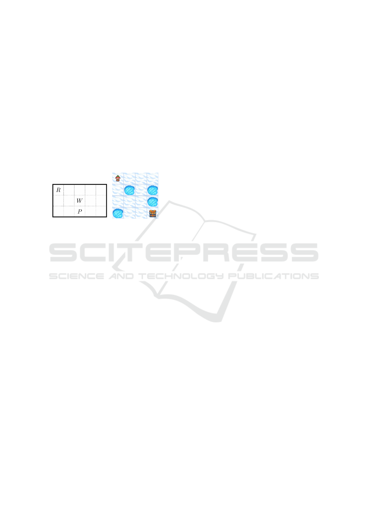
Figure 2: Examples of two commonly used gridworld
games: Classical gridworlds with reward R, walls W and
penalties P as proposed by (Sutton, 1990) and (Crawford
et al., 2018) (left). Example of a 4 × 4 instance of the
gymnasium’s frozen lake environment (Towers et al., 2024)
(right).
Gridworld games as depicted in Fig. 2 are partic-
ularly suitable for QRL benchmarking because their
observation and action spaces naturally map to quan-
tum encodings (one-hot or binary), and unlike Atari
games, which have large state spaces that exceed
current quantum capabilities, gridworld environments
can be scaled appropriately.
In the following we will therefore use established
gridworlds from literature ((Sutton, 1990), (Crawford
et al., 2018) and (M
¨
uller et al., 2021)) as well as
gymnasium’s frozen lake environment for consistent
benchmarking across different studies, addressing the
current issue of fragmented, non-comparable results
in QRL research.
3.2 Metrics
Evaluating and benchmarking QRL algorithms re-
quires incorporating, but also expanding beyond tra-
ditional RL metrics. While current QRL works often
focus solely on performance and sample efficiency,
classical RL highlights the importance of overall
clock time (e.g. in RL methods such as A3C through
asynchronous parameter updates and multi-GPU us-
age (Babaeizadeh et al., 2016)). Therefore, we pro-
pose a set of five metrics, which will be analyzed
across the benchmark environments:
1. performance, assessing the algorithm’s ability to
achieve its objectives
2. sample efficiency, measuring the amount of envi-
ronmental interaction required to reach a certain
performance level (with a predefined maximal en-
vironment step limit)
3. number of circuit executions, highlighting the
costliness of quantum computations
4. quantum clock time, influenced by circuit depth
and quantum hardware
5. qubit scaling, crucial for estimating the future ap-
plicability of the approaches
By examining QRL algorithms through these met-
rics, a better understanding of their strengths, weak-
nesses, and areas for improvement can be gained.
3.3 Evaluating the Q in QRL
The recent work of (Bowles et al., 2024) has empha-
sized a question which has barely been investigated
in QRL: Whether the observed advantages in quan-
tum algorithms stem from quantum principles or other
factors. In this Section we discuss how to answer this
question for the analyzed classes of QRL algorithms.
PQC-QRL: PQCs have been the subject to de-
tailed analyses. Current results suggest that the choice
of ansatz is crucial in order to determine whether the
PQC will suffer from untrainability (also called bar-
ren plateaus (Larocca et al., 2024)) or be classically
simulatable (as has recently been shown for quan-
tum convolutional neural networks (Bermejo et al.,
2024)). To evaluate if the performance of the agents is
due to quantum properties such as entanglement, we
compare the original ansatz of (Skolik et al., 2022)
against two modified versions: For the first modified
ansatz (A), we remove the entangling block, making
the ansatz linearly separable, hence classically simu-
latable. For the second ansatz (B) we do the same but
encode in each qubit the whole state space in the en-
coding block over the layers. By comparing the ansatz
form (Skolik et al., 2022) against these linearly sepa-
rable ansatzes, we can access if the observed perfor-
mance is due to the entanglement.
FE-QRL: While QBM based FE-QRL has shown
promise, with empirical results suggesting its poten-
tial to outperform classical DBM (Crawford et al.,
2018) (also on D-Wave Quantum Annealers (Levit
et al., 2017) and (Neumann et al., 2023)), several
questions remain open. A significant challenge in
FE-QRL is the approximation of the partition func-
tion, which is caused by the limitations of measur-
ing spin configurations of qubits along a fixed axis.
Benchmarking Quantum Reinforcement Learning
777

When a measurement of σ
z
is performed, the quantum
state collapses into one of its eigenstates along the
z-axis, irreversibly destroying any information about
the spin’s projection along the transverse fields di-
rection (represented by σ
x
). Therefore, it remains
questionable, if a Quantum Annealer can be used to
approximate Eq. 5 (Amin, 2015) (Matsuda et al.,
2009) (Venuti et al., 2017). As a result, previous
works have introduced alternative methods to esti-
mate ⟨H
v
⟩. One widely adopted method is called
replica stacking (Levit et al., 2017) (Crawford et al.,
2018), which utilizes the Suzuki-Trotter decompo-
sition (Suzuki, 1976) to construct an approximate
Hamiltonian H
QBM
′
v
. Using the decomposition, the
traverse field term of Eq. 5 is transformed into a clas-
sical Ising model of one dimension higher:
H
QBM
′
v
= −
∑
{h,h
′
}⊆H
r
∑
k=1
θ
hh
′
r
σ
z
hk
σ
z
h
′
k
−
∑
v∈V,h∈H
r
∑
k=1
θ
vh
v
r
σ
z
hk
− w
+

∑
h∈H
r
∑
k=0
σ
z
hk
σ
z
hk+1

,
(11)
where r is the number of replicas, and w
+
=
1
2β
log coth(
Γβ
r
) (Levit et al., 2017). (Suzuki, 1976)
shows, that as the amount of replicas is increased,
the ground state of H
QBM
′
v
converges towards H
QBM
v
.
However, this does not imply ⟨H
QBM
v
⟩ ≈ ⟨H
QBM
′
v
⟩.
Nevertheless, H
QBM
′
v
is used throughout literature to
approximate the free energy of the QBM. This is ei-
ther done with Simulated Annealing, or via a D-Wave
Quantum Annealer. Another problem arises from the
unknown values of Γ and β in the approximation for
H
QBM
′
v
. (Levit et al., 2017) associate a single (aver-
age) virtual Γ to all TFIMs constructed throughout the
FE-QRL. While a validation of this approach is be-
yond the scope of this work, we will proceed with an
empirical evaluation. This evaluation centers on the
following hypothesis, drawn from the aforementioned
studies: If H
QBM
′
v
provides a good approximation of
H
QBM
, we expect superior training performance rela-
tive to the classical H
DBM
v
. To test this hypothesis, we
will examine if the performance of FE-QRL improves
with an increasing number of replicas.
AA-QRL: For this QRL approach we do not con-
duct an additional analysis of its quantum principles,
since in its evaluated form its referred to as QiRL (as
discussed in Section 2.3).
Figure 3: Number of required qubits: For PQC-QRL, the
number of qubits greatly differs between binary and one-hot
state space encoding. For FE-QRL, the number of qubits
depends on the amount of hidden units of the QBM as well
as the number of replicas used for the approximation.
Figure 4: Comparison of different state space encodings on
the 3 ×3 gridworld with an optimal reward of 0.7, indicated
by the dotted black line. The solid lines indicate the mean
over 10 runs and the shaded area indicates the standard de-
viation.
4 RESULTS
We investigate the QRL agents proposed in Section
2 on the gridworld environments proposed in Sec-
tion 3.1: A simple 3 × 3 gridworld as proposed by
(M
¨
uller et al., 2021), a 3 × 5 gridworld as proposed
by (Crawford et al., 2018) and an 4 × 4 as well as
an 8 × 8 instance of the non-slippery frozen lake en-
vironment. The action space for all environments
is chosen to be discrete with four possible actions
(up,down,left,right), which are one-hot encoded for
PQC-QRL and FE-QRL, and binary encoded for AA-
QRL. For the PQC-QRL, we use PQCs with 4, 5, 7
and 9 qubits (depending on the state space of the en-
vironments) with 5 layers each (as depicted in Fig. 1).
For the FE-QRL approach we use two hidden layers
with 4 qubits each. To encode the four actions in the
AA-QRL agent, two qubits are required.
For QPG, we use a learning rate of 0.025 for the
QAIO 2025 - Workshop on Quantum Artificial Intelligence and Optimization 2025
778

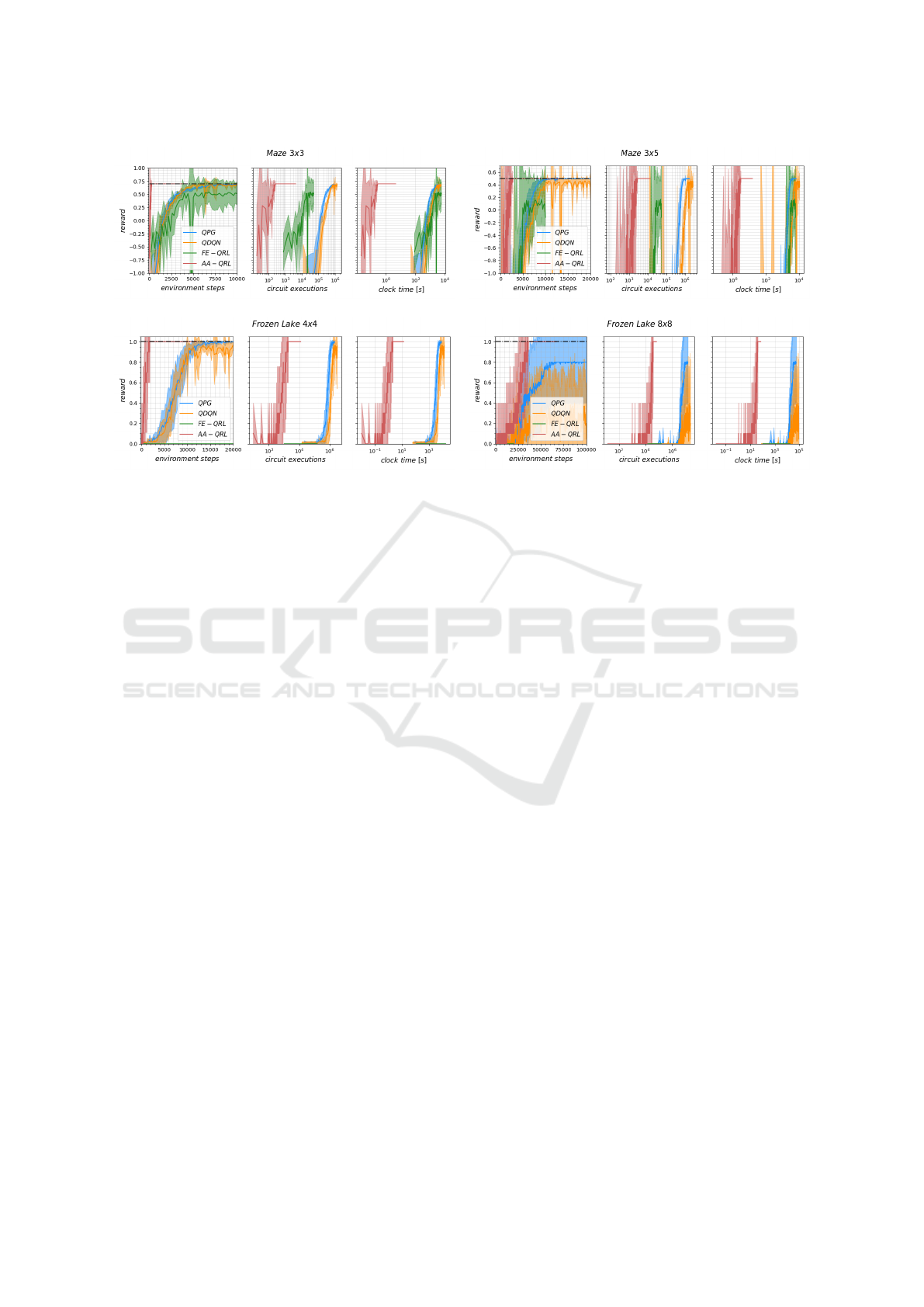
Figure 5: Comparison of the QRL algorithms on four gridworlds. Optimal rewards are indicated by the dotted black line. The
solid lines show the mean over 10 runs and the shaded area the standard deviation.
parameters θ, λ and 0.1 for the output scaling param-
eters w for all environments. For the QDQN, we use a
learning rate of 0.01 for the parameters θ, λ and 0.01
for the output scaling parameters w for all environ-
ments, a γ of 0.95 and an epsilon decay rate from 1
to 0.05. For the simulation of the PQCs we use state
vector simulators.
For the FE-QRL agents, the choice of hyperpa-
rameters is extremely important. Throughout our ex-
periments, slight modification lead to strong fluctua-
tions in performance. Since we do not want to bias
our evaluation and fine tune the algorithms signif-
icantly more than the other algorithms, we do use
learning rate schedules (as proposed by (Crawford
et al., 2018)), but do not fine tune them for the dif-
ferent gridworld environments. Additionally, we use
β = 2.0, Γ = 0.506, and the same γ and epsilon greedy
exploration schedule as for the QDQN agents. To es-
timate ⟨H
QBM
′
v
⟩ we use Simulated Annealing.
As discussed in Section 3.2, we evaluate not only
the performance of the agents in terms of environment
interactions but also with respect to the amount of cir-
cuit executions and quantum clock time. The number
of circuit executions is influenced by both the number
of forward passes and the number of model parame-
ters, particularly in the case of PQC-QRL, since the
parameter-shift rule necessitates a minimum of two
circuit executions per parameter for gradient estima-
tion. Consequently, QDQN agents require a higher
number of circuit executions for the same amount
of environment interactions compared to QPG, as Q-
Learning (in our implementation) revisits previously
seen data through resampling from the replay buffer
more often. For PQC-QRL and AA-QRL, the esti-
mated quantum clock time is derived from assumed
gate times on superconducting hardware of 30ns and
300ns for single and two-qubit gates, respectively, as
well as 300ns measurement times, with 1000 shots.
The estimated quantum clock time for FE-QRL is
based on the usage of the D-Wave Quantum Annealer
Advantage QPU. A single 4 × 4 QBM, approximated
with 5 replicas and with the default anneal schedule
and 1000 shots requires approximately 115ms of QPU
access time.
An important question is whether QRL agents can
scale to larger problem instances. To answer this
question, we need to consider the qubit scaling for
the different approaches. When using one-hot encod-
ing for the state space, the PQC-QRL faces significant
scalability issues, since the number of qubits scales
linearly with the size of the state space (ref. Fig. 3).
For binary encoding on the other hand, this scaling
is significantly better. Note that one needs at least 4
qubits for the one hot encoding of the actions. In con-
trast, FE-QRL’s number of qubits is unaffected by the
encoding method, since the state is represented via the
visible nodes. However, a higher number of visible
nodes (due to the use of one-hot encoding) leads to a
higher number of trainable parameters. The AA-QRL
is insensitive to the encoding scheme, as a separate
quantum circuit is employed for each state, making
the number of required qubits independent of the en-
coding.
In Fig. 4 the comparison of the PQC-QRL algo-
Benchmarking Quantum Reinforcement Learning
779

rithms with binary encoding (4 qubits, 5 layers) and
with one-hot encoding (9 qubits, 5 layers) shows that
even though the number of trainable parameters is
more than twice as high, the performance is compara-
ble in terms of environmental steps. However, due to
the increased number of parameters, the performance
of the larger models is worse in terms of quantum
clock time. On the other hand, the binary encoding
for the FE-QRL agent performs significantly worse
than the one-hot encoded agent, while the clock time
remains the same, since the different encodings only
affect the visible nodes.
In the comparison in Fig. 5 we therefore evaluate
the agents with binary encoding for the PQC-agents
and the one-hot encoded for the FE-QRL agents.
Throughout all gridworlds, the AA-QRL method per-
forms best. This becomes especially apparent for the
quantum clock time of the algorithm. However, as
the size of the gridworlds grow, the method seems to
require proportionally more environment steps (com-
pared to QPG and QDQN). The performance of the
QPG agent and the QDQN agent is similar through-
out the small gridworld sizes. However, for the largest
frozen lake gridworld, the performance is QDQN
starts to deteriorate. The FE-QRL agents are inca-
pable of scaling to the larger frozen lake environ-
ments. While the method has shown promising results
in (Crawford et al., 2018) and other works, it does not
seem to scale well to larger problem instances. The
number of circuit executions is less for the FE-QRL
agents than for the QDQN and QPG agent, but due to
the longer quantum clock times of a single circuit ex-
ecutions, the overall quantum clock times of the two
approaches is comparable.
While all algorithms have the potential to scale up
to problem sizes far beyond the ones utilized in this
work, their performance greatly decreases as problem
sizes grow.
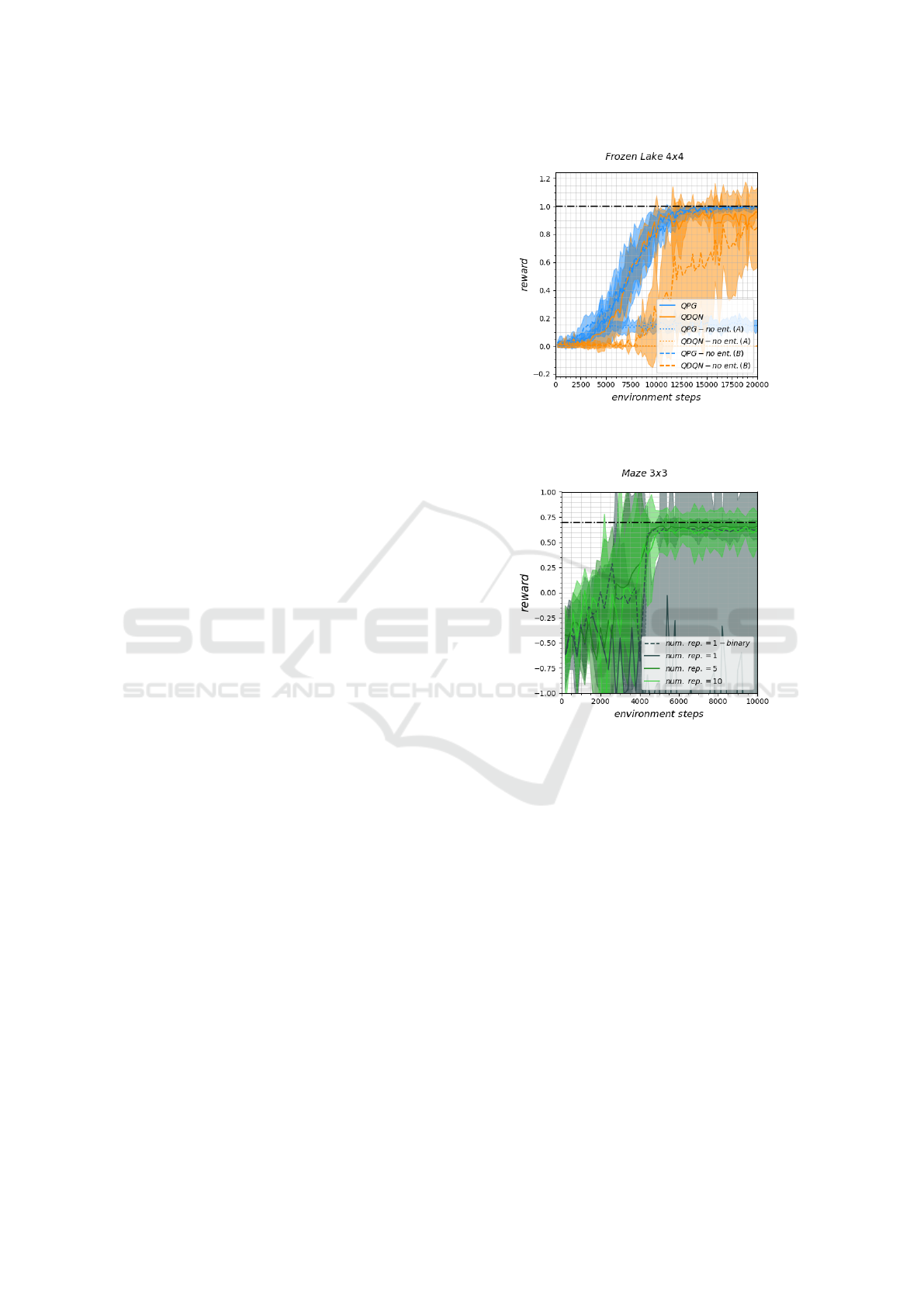
In order to access if the performance of PQC-QRL
relies on quantum properties such as entanglement,
we compare the performance of the proposed ansatz
by (Skolik et al., 2022) against ansatze without any
entangling gates, effectively removing the entangling
blocks (ref. Fig. 1). The results in Fig. 6 show that the
first models without entanglement (A) perform sig-
nificantly worse. This is due to a lack of informa-
tion encoding on the individual qubits. The second
model without entanglement (B) includes all infor-
mation on each qubit, and performs almost identical
for the QDQN agents, but worse for the QPG agents.
The linearly separable ansatze show only partly worse
training performance, and hence the performance of
the quantum algorithm does not seem to mainly rely
on entanglement.
Figure 6: Performance of PQC-QRL algorithms with and
without entanglement on the frozen lake 4 × 4.
Figure 7: Performance of FE-QRL with increasing number
of replicas and binary and onehot encoding on the 3 × 3
gridworld.
We compare the performance of the FE-QRL ap-
proach for an increasing numbers of replicas via sim-
ulated Annealing: 1 (so a classical DBM), 5 and 10.
We also evaluate the classical DBM with binary and
onehot encoding. As discussed in Section 3.3, we
would expect that an increase of the number of repli-
cas would result in better training performance, if the
performance of the QBM relies on quantum princi-
ples. However, as we can see in Fig. 7, we see no such
correlation. While the set of hyperparameters does
not lead to good performance for the onehot encoded
classical DBM, the performance of the FE-QRL with
5 and 10 replicas is comparable to the binary encoded
DBM. Hence, the performance of the FE-QRL ap-
proach seems to rely too strongly on hyperparameters,
making a meaningful ranking unfeasible.
QAIO 2025 - Workshop on Quantum Artificial Intelligence and Optimization 2025
780

5 DISCUSSION
In this study, we conducted a comprehensive evalua-
tion of three QRL classes (PQC-QRL with QPG and
QDQN, FE-QRL and AA-QRL). Our evaluation ex-
tends beyond previous works by the number of con-
sidered QRL algorithms and the incorporation of ad-
ditional metrics such as circuit executions and quan-
tum clock time, providing a more holistic and realistic
assessment of these algorithms’ practical feasibility.
For PQC-QRL, we observed only a minor depen-
dence on quantum entanglement, with performance
deteriorating only slightly when entanglement was re-
moved. Interestingly, our investigation of FE-QRL
showed no clear correlation between performance
and the number of replicas used to approximate the
Hamiltonian of the QBM H
QBM
v
, but rather a great
dependence on hyperparameters. These findings sug-
gest that most QRL approaches may not greatly rely
on their quantum components.
QRL, particularly when applied to gridworld
games, demonstrates promising scalability to larger
problems through binary encoding, even with cur-
rent hardware limitations. However, the algorithms
we evaluated still require substantial improvement to
achieve competitive performance levels. Our work
can serve as an underlying benchmarking reference
for this future development.
Future work should aim to include the evalua-
tion of noise resilience as an additional metric in or-
der to assess these algorithms’ practical viability in
real quantum hardware implementations. Addition-
ally, not only the quantum clock time, but also the
overall clock time of these hybrid algorithms should
be considered when comparing QRL to classical RL.
CODE AVAILABILITY
The code to reproduce the results as well as the data
used to generate the plots in this work can be found
here: https://github.com/georgkruse/cleanqrl
ACKNOWLEDGEMENTS
The research is part of the Munich Quantum Valley,
which is supported by the Bavarian state government
with funds from the Hightech Agenda Bayern Plus.
REFERENCES
Abbas, A., Sutter, D., Zoufal, C., Lucchi, A., Figalli, A.,
and Woerner, S. (2021). The power of quantum neural
networks. Nature Computational Science, 1(6):403–
409.
Ackley, D. H., Hinton, G. E., and Sejnowski, T. J. (1985). A
learning algorithm for boltzmann machines. Cognitive
science, 9(1):147–169.
Amin, M. H. (2015). Searching for quantum speedup in
quasistatic quantum annealers. Physical Review A,
92(5):052323.
Amin, M. H., Andriyash, E., Rolfe, J., Kulchytskyy, B.,
and Melko, R. (2018). Quantum boltzmann machine.
Physical Review X, 8(2):0541.
Babaeizadeh, M., Frosio, I., Tyree, S., Clemons, J., and
Kautz, J. (2016). Reinforcement learning through
asynchronous advantage actor-critic on a gpu. arXiv
preprint arXiv:1611.06256.
Bermejo, P., Braccia, P., Rudolph, M. S., Holmes, Z., Cin-
cio, L., and Cerezo, M. (2024). Quantum convo-
lutional neural networks are (effectively) classically
simulable. arXiv preprint arXiv:2408.12739.
Bowles, J., Ahmed, S., and Schuld, M. (2024). Bet-
ter than classical? the subtle art of benchmarking
quantum machine learning models. arXiv preprint
arXiv:2403.07059.
Chen, S. Y.-C., Yang, C.-H. H., Qi, J., Chen, P.-Y., Ma,
X., and Goan, H.-S. (2020). Variational quantum cir-
cuits for deep reinforcement learning. IEEE access,
8:141007–141024.
Coelho, R., Sequeira, A., and Paulo Santos, L. (2024). Vqc-
based reinforcement learning with data re-uploading:
performance and trainability. Quantum Machine In-
telligence, 6(2):53.
Crawford, D., Levit, A., Ghadermarzy, N., Oberoi, J. S.,
and Ronagh, P. (2018). Reinforcement learning using
quantum boltzmann machines. Quantum Information
& Computation.
Dong, D., Chen, C., Chu, J., and Tarn, T.-J. (2010).
Robust quantum-inspired reinforcement learning for
robot navigation. IEEE/ASME transactions on mecha-
tronics, 17(1):86–97.
Dong, D., Chen, C., Li, H., and Tarn, T.-J. (2008). Quan-
tum reinforcement learning. IEEE Transactions on
Systems, Man, and Cybernetics, Part B (Cybernetics),
38(5):1207–1220.
Dr
˘
agan, T.-A., Monnet, M., Mendl, C. B., and Lorenz, J. M.
(2022). Quantum reinforcement learning for solv-
ing a stochastic frozen lake environment and the im-
pact of quantum architecture choices. arXiv preprint
arXiv:2212.07932.
Hu, Y., Tang, F., Chen, J., and Wang, W. (2021). Quantum-
enhanced reinforcement learning for control: A pre-
liminary study. Control Theory and Technology,
19:455–464.
Jerbi, S., Gyurik, C., Marshall, S., Briegel, H., and Dunjko,
V. (2021a). Parametrized quantum policies for rein-
forcement learning. Advances in Neural Information
Processing Systems, 34:28362–28375.
Benchmarking Quantum Reinforcement Learning
781

Jerbi, S., Trenkwalder, L. M., Poulsen Nautrup, H., Briegel,
H. J., and Dunjko, V. (2021b). Quantum enhance-
ments for deep reinforcement learning in large spaces.
PRX Quantum, 2(1).
Kappen, H. J. (2020). Learning quantum models from quan-
tum or classical data. Journal of Physics A: Mathe-
matical and Theoretical, 53(21):214001.
Kruse, G., Coehlo, R., Rosskopf, A., Wille, R., and Lorenz,
J. M. (2024). Hamiltonian-based quantum reinforce-
ment learning for neural combinatorial optimization.
arXiv preprint arXiv:2405.07790.
Kruse, G., Dragan, T.-A., Wille, R., and Lorenz, J. M.
(2023). Variational quantum circuit design for quan-
tum reinforcement learning on continuous environ-
ments. arXiv preprint arXiv:2312.13798.
Larocca, M., Thanasilp, S., Wang, S., Sharma, K., Bia-
monte, J., Coles, P. J., Cincio, L., McClean, J. R.,
Holmes, Z., and Cerezo, M. (2024). A review of bar-
ren plateaus in variational quantum computing. arXiv
preprint arXiv:2405.00781.
Levit, A., Crawford, D., Ghadermarzy, N., Oberoi, J. S.,
Zahedinejad, E., and Ronagh, P. (2017). Free energy-
based reinforcement learning using a quantum proces-
sor. arXiv preprint arXiv:1706.00074.
Matsuda, Y., Nishimori, H., and Katzgraber, H. G. (2009).
Ground-state statistics from annealing algorithms:
quantum versus classical approaches. New Journal of
Physics, 11(7):073021.
Meyer, N., Ufrecht, C., Periyasamy, M., Scherer, D. D.,
Plinge, A., and Mutschler, C. (2022). A survey
on quantum reinforcement learning. arXiv preprint
arXiv:2211.03464.
M
¨
uller, T., Roch, C., Schmid, K., and Altmann, P.
(2021). Towards multi-agent reinforcement learning
using quantum boltzmann machines. arXiv preprint
arXiv:2109.10900.
Neumann, N. M. P., de Heer, P. B. U. L., and Phillipson, F.
(2023). Quantum reinforcement learning - comparing
quantum annealing and gate-based quantum comput-
ing with classical deep reinforcement learning. Quan-
tum Information Processing, 22(2).
Sallans, B. and Hinton, G. E. (2004). Reinforcement learn-
ing with factored states and actions. The Journal of
Machine Learning Research, 5:1063–1088.
Skolik, A., Jerbi, S., and Dunjko, V. (2022). Quantum
agents in the gym: a variational quantum algorithm
for deep q-learning. Quantum, 6:720.
Skolik, A., Mangini, S., B
¨
ack, T., Macchiavello, C., and
Dunjko, V. (2023). Robustness of quantum reinforce-
ment learning under hardware errors. EPJ Quantum
Technology, 10(1):1–43.
Sutton, R. S. (1990). Integrated architectures for learning,
planning, and reacting based on approximating dy-
namic programming. In Machine learning proceed-
ings 1990, pages 216–224. Elsevier.
Suzuki, M. (1976). Relationship between d-dimensional
quantal spin systems and (d+ 1)-dimensional ising
systems: Equivalence, critical exponents and sys-
tematic approximants of the partition function and
spin correlations. Progress of theoretical physics,
56(5):1454–1469.
Towers, M., Kwiatkowski, A., Terry, J., Balis, J. U.,
De Cola, G., Deleu, T., Goulao, M., Kallinteris, A.,
Krimmel, M., KG, A., et al. (2024). Gymnasium: A
standard interface for reinforcement learning environ-
ments. arXiv preprint arXiv:2407.17032.
Venuti, L. C., Albash, T., Marvian, M., Lidar, D., and Za-
nardi, P. (2017). Relaxation versus adiabatic quan-
tum steady-state preparation. Physical Review A,
95(4):042302.
QAIO 2025 - Workshop on Quantum Artificial Intelligence and Optimization 2025
782