Improving Underwater Ship Sound Classification with CNNs and
Advanced Signal Processing
Pedro Guedes
1 a
, Jos
´
e Franco Amaral
1 b
, Thiago Carvalho
1,2 c
and Pedro Coelho
1 d
1
FEN/UERJ, Rio de Janeiro State University, Rio de Janeiro, Brazil
2
Electrical Engineering Department, Pontifical Catholic University of Rio de Janeiro, Rio de Janeiro, Brazil
Keywords:
Neural Networks, Signal Processing, Wavelet Transforms, Underwater Signals, Convolutional Neural
Networks.
Abstract:
The identification of underwater sound patterns has become an area of great relevance, both in marine biol-
ogy, for studying species, and in the identification of ships. However, the significant presence of noise in the
underwater environment poses a technical challenge for the accurate classification of these signals. This work
proposes the use of signal analysis techniques, such as Mel Frequency Cepstral Coefficients (MFCCs) and
Wavelet Transform, combined with Convolutional Neural Networks (CNNs), for classifying ship audio cap-
tured in a real-world environment strongly influenced by its surroundings. The developed models achieved a
better accuracy in signal classification, demonstrating robustness in the face of adverse underwater conditions.
The results indicate the effectiveness of the proposed approach, contributing to advances in the application of
neural network techniques to underwater sound signals.
1 INTRODUCTION
The use of audio signal classification techniques has
been widely explored in underwater environments. In
the biological field (Hamard et al., 2024), for instance,
these techniques are extensively used to study marine
life. They play a crucial role in the conservation of en-
dangered species, enabling the identification of sound
patterns associated with specific behaviors, such as
feeding or migration (Hamard et al., 2024). Further-
more, they assess the impact of human activities as a
stressor for ocean fauna (F. Traverso et al., 2024). Ad-
ditionally, these techniques are applied to the study of
natural phenomena, such as geological events (Bel-
ghith et al., 2018), and are highly relevant for mili-
tary purposes in the passive identification of vessels
(Ahmada et al., 2024), allowing target identification
without exposing the observer’s position.
Despite their importance, the classification task
in underwater environments faces unique challenges.
The marine environment is characterized by a high
density of ambient noise, including sounds gener-
ated by waves, marine animals, and human activities.
Moreover, the strong attenuation and absorption of
sound in aquatic media result in signals intercepted by
a
https://orcid.org/0009-0005-8200-8448
b
https://orcid.org/0000-0003-4951-8532
c
https://orcid.org/0000-0001-8689-1438
d
https://orcid.org/0000-0003-3623-1313
hydrophones that often exhibit significant distortions.
Traditional passive classification methods require
expert knowledge. However, their accuracy is limited
due to the complexity of the marine environment (He
et al., 2024). Consequently, traditional machine learn-
ing (ML) techniques, such as Support Vector Ma-
chines (SVM) and Random Forests (RF) (Dong et al.,
2022), have been employed. However, these methods
often perform poorly in noisy environments, which
are common in underwater settings.
More recently, Neural Network (NN) models have
been widely used jointly with signal processing tech-
niques, as this combination exhibits strong perfor-
mance even in noise-saturated environments.
In this study, we explore time-frequency analy-
sis techniques, combined with Convolutional Neural
Networks (CNNs), to classify ships based on acoustic
signals captured by hydrophones. The contributions
are three-fold:
• We propose an strategy to combine signal pro-
cessing methods and CNNs to classify the ships
in the underwater area.
• We conducted experiments to evaluate the pro-
posed strategy with respect to previous method-
ologies applied to this work.
• We evaluated the effects of the signal processing
methods applied in this work to gather insights
from the proposed approach.
Guedes, P., Amaral, J. F., Carvalho, T. and Coelho, P.
Improving Underwater Ship Sound Classification with CNNs and Advanced Signal Processing.
DOI: 10.5220/0013418300003929
Paper published under CC license (CC BY-NC-ND 4.0)
In Proceedings of the 27th International Conference on Enterprise Information Systems (ICEIS 2025) - Volume 1, pages 555-561
ISBN: 978-989-758-749-8; ISSN: 2184-4992
Proceedings Copyright © 2025 by SCITEPRESS – Science and Technology Publications, Lda.
555

The remainder of this article is organized as fol-
lows. Section 2 presents a literature review of re-
lated works, highlighting the most commonly used
approaches that can be applied to ship classification.
Section 3 outlines the methodology, including data
collection, preprocessing, and the methods used for
classification. In Section 4 we discussed how the data
acquisition was carried out, the classification tech-
niques used, and the protocol for our experiment. The
results are discussed in Section 5. Finally, the conclu-
sion is presented in Section 6.
2 LITERATURE REVIEW
As presented in Section 1, several works have used
ML and DL techniques to classify audio signals in ad-
verse environments, aiming to overcome challenges
such as background noise, attenuation, and the over-
lap of sound sources.
Traditional machine learning methods, such as
SVM and RF, have been widely used in early works
due to their simplicity and effectiveness on smaller
datasets. These methods rely on manual feature
extraction, which can be performed through time-
frequency analysis, such as using spectrograms. For
example, (Ahmada et al., 2023) applied SVM to clas-
sify marine sounds, achieving a Precision of 82%
on a dataset containing sounds from different ma-
rine species. The model was reportedly effective
in environments with moderate noise, but degraded
in high-noise scenarios. Also, (Liang et al., 2024)
used RF for identifying underwater geological events.
The approach achieved a Precision of 75% on highly
distorted signals, highlighting the robustness of the
method for limited datasets.
Despite their simplicity, these techniques face dif-
ficulties in extracting relevant features from noisy
data, requiring better data preprocessing before clas-
sification. For example, (Ahmada et al., 2024) im-
plemented CNNs to classify vessel sounds based on
spectrograms. The model achieved a Precision of
92%, demonstrating excellent performance in envi-
ronments with moderate noise.
Recently, one of the main approaches for sig-
nal classification is based on a mixture of signal
processing methods and computer vision models.
Therefore, the use of time-frequency representations,
such as spectrograms and scalograms, has been key
to improving classifier performance. For example,
(F. Traverso et al., 2024) used scalograms generated
by Continuous Wavelet Transform (CWT) to iden-
tify shipment sound patterns, achieving an accuracy
of 89% when combining the representations with con-
volutional networks. Additionaly, (Gencoglu et al., )
demonstrated that log-Mel spectrograms, when used
as input for CNNs, resulted in a 10% increase in Pre-
cision compared to traditional linear spectrograms.
3 PROPOSED APPROACH
In this section, we present the proposed approach for
ship classification. Our pipeline, illustrated in Figure
1 creates a visual representation of the signal, which
is then used in a CNN.
3.1 Preprocessing: Time-Frequency
Analysis
The time-frequency analysis, aimed at extracting rep-
resentative features from the obtained underwater
acoustic signals, inspired by the flowchart presented
in Figure 2.
Due to the cyclic nature of the sounds from the
machinery and propeller of a ship, the audio signals
were segmented into 5-second intervals, as described
in previous works highlighting the effectiveness of
segmentation for capturing local temporal variations
(Hamard et al., 2024), essential for acoustic pattern
analysis and expanding the use of the dataset.
Among the extracted features, Mel-Frequency
Cepstral Coefficients (MFCCs) play a central role.
MFCCs represent the spectral features of the signal
on a Mel scale, which models human auditory per-
ception. To calculate the MFCCs, the signal is ini-
tially decomposed using the Fourier Transform (FT),
represented as:
X(k) =
N−1
∑
n=0
x(n)e
−j
2πkn
N
, (1)
where x(n) is the input signal, N is the total number
of samples, and k represents the frequency index. The
resulting power spectrum is mapped to a Mel scale,
with bands distributed logarithmically. The extraction
of MFCCs includes the calculation of deltas (first dif-
ferences) and accelerations (second differences), de-
fined as:
∆c
t
=
∑
N
n=1
n ·(c
t+n
−c
t−n
)
2
∑
N
n=1
n
2
, (2)
where c
t
represents the coefficient in t, and N is the
calculation window. This approach captures the sig-
nal trending, which is useful to discriminate acoustic
events in short-time duration.
ICEIS 2025 - 27th International Conference on Enterprise Information Systems
556

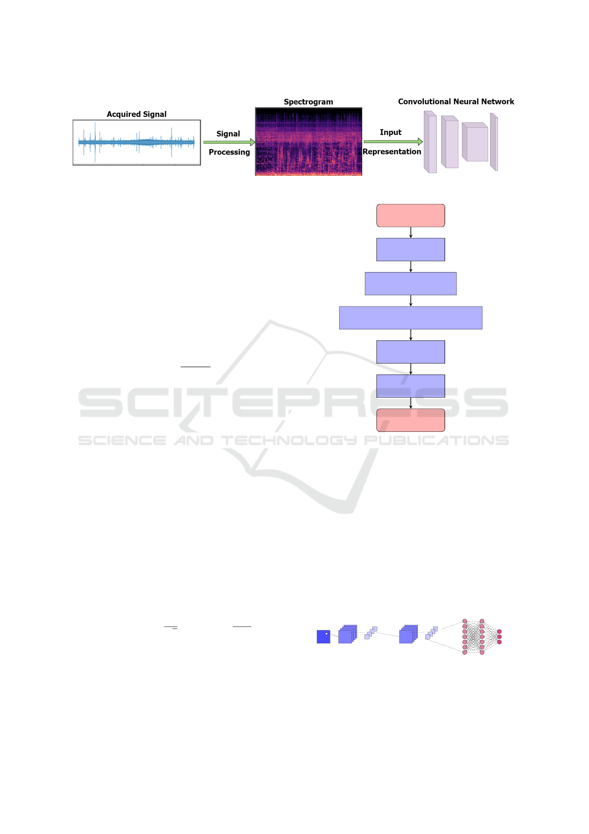
Figure 1: Pipeline for the proposed solution.
The Short Time Fourier Transform (STFT) is ap-
plied to decompose the signal in frequency signals
along the time. The STFT is defined as:
ST FT {x(t)}(τ, ω) =
Z
∞
−∞
x(t)w(t −τ)e
−jωt
dt , (3)
where w(t) is the window function, τ
´
e o tempo-
ral displacement, and ω represents the angular fre-
quency. The STFT allows the spectrogram develop-
ment, while the Power Spectrum Density (PSD) is
obtained to quantitatively measure the power distri-
bution in each frequency:
PSD( f ) =
|X( f )|
2
T
, (4)
where X( f ) represents the frequency spectrum and T
the segment duration.
To enhance the perception of dominant frequen-
cies, the Log-Mel Spectrogram was used, highlight-
ing the most relevant frequencies and representing the
acoustic signatures specific to each class of ship. The
values were then converted to a decibel (dB) scale to
normalize the data and enhance small amplitude vari-
ations, making subtle differences more perceptible:
S
Mel
(m) = 10 ·log
10
K
∑
k=1
|X(k)|
2
H
m
(k)
!
, (5)
where H
m
(k) is the Mel filter Response in band m, and
K is the number of filters.
Additionally, the Continuous Wavelet Transform
(CWT), using the Morlet wavelet, was applied to
capture temporal and spectral variations at different
scales. The CWT is given by:
CW T {x(t)}(a, b) =
1
√
a
Z
∞
−∞
x(t)ψ
∗

t −b
a

dt ,
(6)
where ψ(t) is the wavelet function, a is the scaling
factor, b is the displacement parameter, and ψ
∗
de-
notes the conjugate of the wavelet.
All features were normalized to ensure uniformity
among the extracted values, eliminating scale dif-
ferences and ensuring better classification efficiency.
Begin
Load Audio
Segment audio (5 seconds)
Extract Features (MFCC, STFT, PSD, etc.)
Appliy CWT
Normalize Fatures
Save dataset
Figure 2: Temporal-frequency analysis applied in this work.
The integration of these techniques provided a ro-
bust set of features, widely used in the literature, suit-
able for the analysis and classification of underwater
acoustic signals.
3.2 Convolutional Neural Network
The Figure 3 shows the architecture of a CNN. For the
case under study, the input consists of the processed
audio data from the ship classes we aim to classify.
In other words, the CNN was designed to perform the
classification of sequential data, as discussed in Sec-
tion 3.1.
Input
Conv1D
Pooling
Conv1D
Pooling
Dense 1 Dense 2
Output
Figure 3: 1D Convolutional Neural Network Architecture.
Thus, the CNN we use is a 1D-CNN, composed
of convolution, pooling, and dropout layers, as well
as two fully connected layers.
Improving Underwater Ship Sound Classification with CNNs and Advanced Signal Processing
557

4 EXPERIMENTS
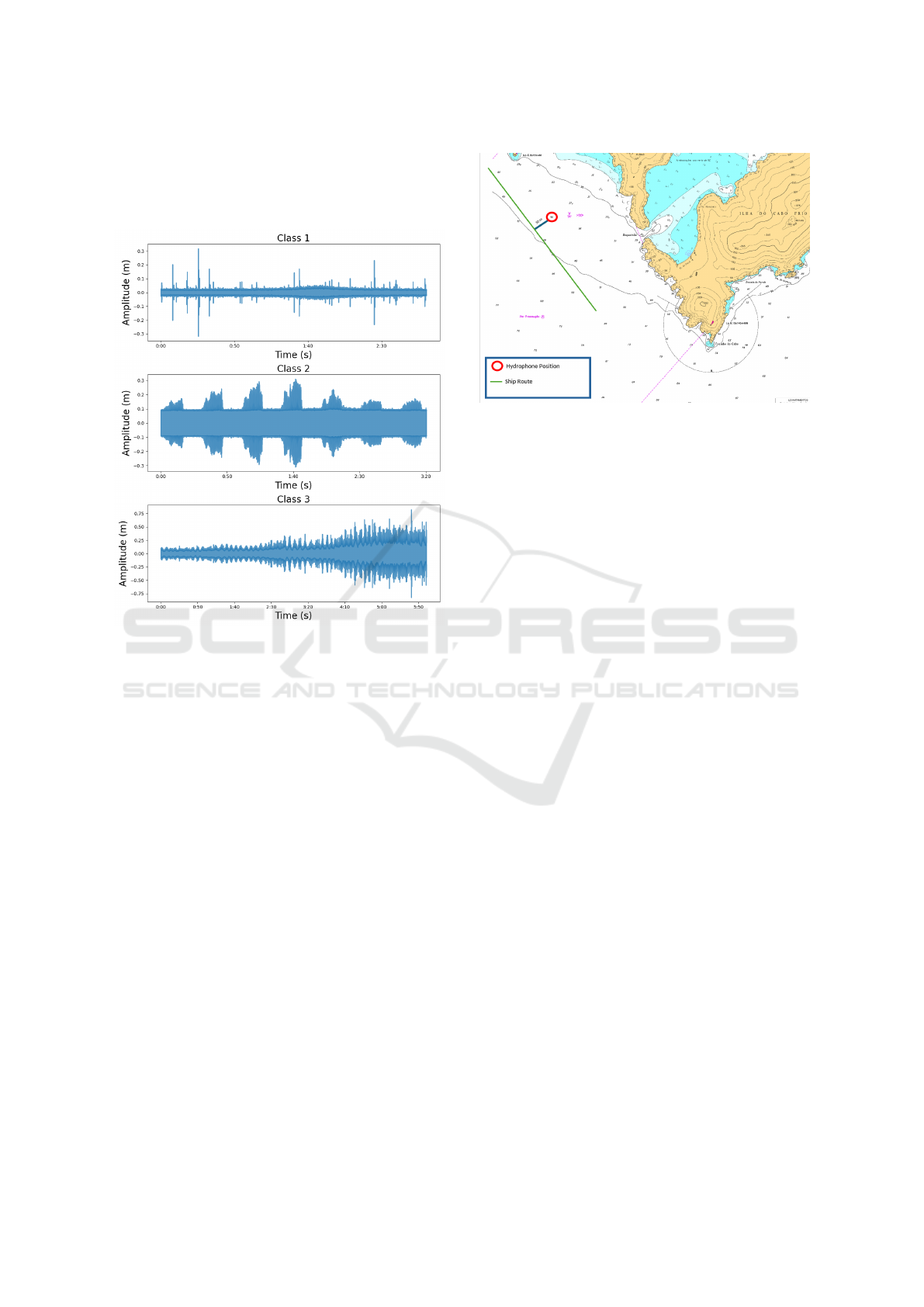
4.1 Data Acquisition
Figure 4: Example of the acoustic signature of ship classes.
The underwater acoustic data analyzed here
comes from 13 ships, which are grouped into three
classes. In Figure 4, examples of the acoustic signa-
tures of these classes are presented.
The recordings were carried out in two scenarios:
static, with the ship anchored and onboard equipment
turned on, and dynamic, with the ship in motion. The
data were collected near Ilha do Cabo Frio (Arraial do
Cabo, Brazil), with coordinates Latitude: 22°58’00”
S and Longitude: 41°59’00” W. A single hydrophone
was used for the recordings.
As shown in Figure 5, the depth of the location is
40 meters, and the hydrophone was positioned 4 me-
ters above the seafloor, i.e., at a depth of 36 meters.
The shortest distance between the ships’ route and the
hydrophone position was 50 meters, which helped to
minimize signal dispersion and to reduce the interfer-
ence.
These problems suffers from a class imbalance,
with 2179 samples for Class 1, 3427 samples for
Class 2 and 2530 samples for Class 3. We opt for the
the undersampling technique, meaning that the ma-
jority classes (with more samples) were reduced to
match the number of samples in the minority class,
ensuring that all classes have the same number of
samples, eliminating imbalance and reducing bias in
Figure 5: Data Acquisition displacement.
learning models.
4.2 Classification Techniques Used
The techniques chosen for classifying the audio can
be divided into two methods: ML and CNN. These
techniques were selected due to their widespread use
in the literature for problems of this type, as can be
seen in (Chalmers et al., 2021) and (Ahmada et al.,
2024), for example. The following techniques were
chosen for this classical approach:
• K-NN: This unsupervised learning algorithm was
used as an initial step to explore the data struc-
ture. The goal was to group the data into three
clusters corresponding to the ship classes. Using
K-NN allows patterns and similarities in the data
to be identified without requiring labels, serving
as a basis for later comparisons with supervised
methods.
In this study, we used centroid initialization due to
its fast convergence. Fifty initializations were per-
formed to ensure result robustness, with each ini-
tialization having a maximum of 500 iterations. A
tolerance of 10
−6
for centroid movement between
iterations was adopted as the stopping criterion.
• Random Forest: This supervised classifier was
chosen for its robustness in handling noisy and
non-linearly separable data. In order to balance
time and accuracy, we used 100 trees in the en-
semble. The splitting criterion chosen was Gini,
which measures node purity. For maximum depth,
we opted not to impose a limit. Bootstrapping was
applied.
• Support Vector Machines: This classifier was
selected to maximize the separation between
classes. To handle non-linearly separable data,
an RBF (Radial Basis Function) kernel was em-
ICEIS 2025 - 27th International Conference on Enterprise Information Systems
558

ployed, mapping the data to a higher-dimensional
space, with standard regularization (C = 1).
• Logistic Regression: As a baseline model, Mul-
ticlass Logistic Regression was employed due to
its simplicity and efficiency. This method allows
modeling the probability of a sample belonging to
a specific class using the logistic function.
For this case, a maximum of 500 iterations and
standard regularization were used.
4.3 Experimental Protocol
All cases addressed in this study were standardized,
and the PCA was employed to reduce the data dimen-
sionality to 10 principal components, which captured
100% of the variance. The data was split as follows:
70% for training, 20% for validation, and 10% for
testing.
For the proposed approach, we trained the CNN
from scratch. For the first convolutional layer, 32 fil-
ters were used; for the second, 64 filters were em-
ployed, allowing the learning of more complex and
high-level patterns in the feature maps generated by
the first layer. The ReLU activation function was used
in both layers. We also applied a 1D MaxPooling and,
the hidden dense layer consisted of 128 neurons with
a dropout of 30%. The Adam optimizer was used with
a learning rate of 0.001, and Categorical Crossentropy
as the loss function.
In this work, we evaluated the results in terms
of traditional classification metrics, such as accuracy.
Since the dataset is balanced, for the F1-Score, Preci-
sion, and Recall metrics, we reported the macro aver-
age on the test set.
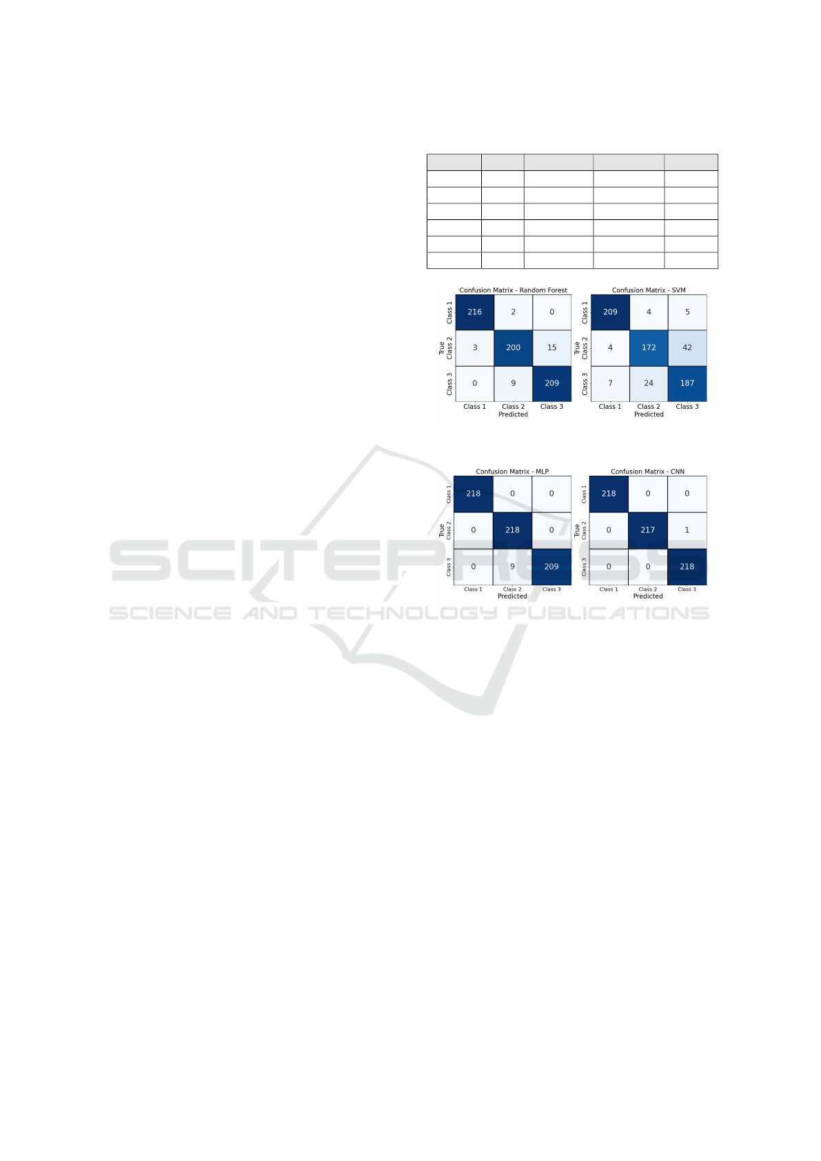
5 DISCUSSION AND RESULTS
To evaluate the proposed techniques, we generated
a report with the metrics presented in Table 1. The
KNN model, which showed the worst performance,
with accuracy lower than the na
¨
ıve model (33.3%).
This result underscores the inability of this technique
to properly separate the data, reflecting significant
overlap between classes 2 and 3 and considerable con-
fusion between classes 1 and 2, with 53 errors.
The SVM and RF techniques, on the other hand,
delivered more robust results, as shown in 6. The
SVM exhibited better results if we analyze the classes
2 and 3, indicating that these classes have features that
are not completely separable in the feature space.
The LR, as expected for being a linear model,
showed moderate performance, highlighting its lim-
Table 1: Results for Ship Classification.
Model Acc. F1-Score Precision Recall
KNN 0.10 0.08 0.20 0.08
RF 0.96 0.96 0.96 0.96
SVM 0.87 0.87 0.87 0.87
LR 0.71 0.71 0.71 0.71
MLP 0.99 0.99 0.99 0.99
CNN 1.00 1.00 1.00 1.00
Figure 6: Confusion matrix for Random Forest and SVM
models.
Figure 7: Confusion Matrix for MLP and CNN.
itation in problems with more complex decision
boundaries.
As shown in Table 1, the MLP and CNN tech-
niques delivered excellent results on the test set,
demonstrating that both are capable of learning rel-
evant patterns in the data.
However, the CNN shows better efficiency, con-
verging more quickly and exhibiting more stable gen-
eralization to the validation set, as observed in the fig-
ure. In contrast, the MLP presented some classifica-
tion errors, as shown in Figure 7.
The absence of significant discrepancies between
training and validation losses suggests that neither
technique shows signs of overfitting on the validation
set, as illustrated in FIgure 8.
5.1 Ablation Study: Effects of Signal
Processing Methods
To identify which techniques used for signal process-
ing were most relevant for a marine environment with
a cyclic audio signal, we conducted the experiments
Improving Underwater Ship Sound Classification with CNNs and Advanced Signal Processing
559

Figure 8: Loss function for MLP and CNN models.
to validate the strenght of the signal processing used
in this work.
5.1.1 Removing the MFCC Delta
Firstly, we removed the delta from the MFCC to ver-
ify whether, even in the case of audio capture in an un-
controlled environment—i.e., an environment subject
to unpredictable noise from marine organisms, ocean
currents, other vessels, and other types of random in-
terference—the results would be affected. The results
presented in Table 2 were obtained for the test set.
Table 2: Results for Ship Classification without MFCC
Delta.
Model Acc. F1-Score Precision Recall
KNN 0.10 0.08 0.20 0.08
RF 0.96 0.96 0.96 0.96
SVM 0.87 0.87 0.87 0.87
LR 0.72 0.72 0.72 0.72
MLP 0.99 0.99 0.99 0.99
CNN 1.00 1.00 1.00 1.00
Upon analyzing the results, we found that remov-
ing the delta technique from the MFCC did not affect
the outcomes. This indicates that the rapid temporal
changes captured by the technique are likely associ-
ated only with noise. In other words, the patterns re-
quired for ship classification can be captured solely
by the static MFCCs.
5.1.2 Removing the PSD
By removing the PSD technique, we aimed to un-
derstand whether the studied ship classes have dis-
tinct energy signatures at specific frequencies, mak-
ing PSD a relevant technique, or if it is merely captur-
ing low-frequency noise inherent to the underwater
environment. The results presented in Table 3 were
obtained for the test set.
In this case, we observed an improvement in the
results of the ML techniques, particularly in SVM and
LR. This indicates that the PSD was capturing under-
water background noise, which is irrelevant for ship
classification. Its removal reduced the dimensionality
Table 3: Results for Ship Classification without PSD.
Model Acc. F1-Score Precision Recall
KNN 0.23 0.18 0.20 0.16
RF 0.98 0.98 0.98 0.98
SVM 0.93 0.93 0.93 0.93
LR 0.81 0.81 0.81 0.81
MLP 0.99 0.99 0.99 0.99
CNN 1.00 1.00 1.00 1.00
of the problem, improving the generalization capabil-
ity of SVM and LR.
The indifference in the results for neural network-
based models demonstrates their ability to automati-
cally filter noise and redundancies. Another important
conclusion is that the underwater environment likely
contains dominant noise at specific frequencies. This
could be useful for studies on biodiversity and geo-
logical events. For the study in question, analyzing
and filtering such noise during preprocessing could
benefit the ML models.
6 CONCLUSION
In this work, we successfully established a pipeline
for preprocessing underwater audio captured in an un-
controlled environment. We also developed an ap-
proach based on CNN, which were capable of effec-
tively distinguishing between the three ship classes,
achieving 100% accuracy, precision, and F1-score
without overfitting.
This field of study holds significant potential
across various domains, including biology, geology,
and military applications. The techniques and pre-
processing methods developed in this work can be
adapted to other types of problems, such as identi-
fying seabed sediments or even detecting underwater
objects.
As a proposal for future work, we could attempt
to differentiate whether a ship is anchored or in mo-
tion based on the audio signals it emits. This could be
highly valuable for military or law enforcement activ-
ities. In addition, we plan to extend this study to a
broader area of data acquisition, with the objective of
identifying more classes of ships in different scenar-
ios. This new test might be able to evaluate the robust-
ness and the generalization capability of the proposed
approach.
ICEIS 2025 - 27th International Conference on Enterprise Information Systems
560

ACKNOWLEDGEMENTS
This work was supported in part by the Coordenac¸
˜
ao
de Aperfeic¸oamento de Pessoal de N
´
ıvel Superior -
Brasil (CAPES) - Finance Code 001, Conselho Na-
cional de Desenvolvimento e Pesquisa (CNPq) un-
der Grant 140254/2021-8, and Fundac¸
˜
ao de Amparo
`
a Pesquisa do Rio de Janeiro (FAPERJ)
REFERENCES
Ahmada, F., Ansaria, M. Z., Anwara, R., Shahzada, B., and
Ikrama, A. (2023). Deep learning based classification
of underwater acoustic signals. In International Con-
ference on Machine Learning and Data Engineering
(ICMLDE 2023), pages 1115–1124. Elsevier.
Ahmada, F., Ansaria, M. Z., Anwara, R., Shahzada, B., and
Ikrama, A. (2024). Spectral analysis of the underwa-
ter acoustic noise radiated by ships with controllable
pitch propellers. Ocean Engineering, 115112(299):1–
14.
Belghith, E. H., Rioult, F., and Bouzidi, M. (2018). Acous-
tic diversity classifier for automated marine big data
analysis. In IEEE 30th International Conference
on Tools with Artificial Intelligence, pages 130–136.
IEEE.
Chalmers, C., Fergus, P., Wich, S., and Longmore, S. N.
(2021). Modelling animal biodiversity using acous-
tic monitoring and deep learning. Proceedings of the
IEEE International Workshop.
Dong, Y., Shen, X., Yan, Y., and Wang, H. (2022). Small-
scale data underwater acoustic target recognition with
deep forest model. In IEEE International Conference
on Signal Processing, Communications and Comput-
ing (ICSPCC). IEEE.
F. Traverso, T. G., Rizzuto, E., and A.Trucco (2024). Under-
water noise characterization of a typical fishing vessel
from atlantic canada. Ocean Engineering, pages 1–6.
Gencoglu, O., Virtanen, T., and Huttunen, H. Recognition
of acoustic events using deep neural networks. pages
1–5.
Hamard, Q., Pham, M.-T., Cazau, D., and Heerah, K.
(2024). A deep learning model for detecting and clas-
sifying multiple marine mammal species from passive
acoustic data. Ecological Informatics, 115112(84):1–
19.
He, J., Zhang, B., Liu, P., Li, X., Wang, L., and Tang, R.
(2024). Effective underwater acoustic target passive
localization of using a multi-task learning model with
attention mechanism: Analysis and comparison un-
der real sea trial datasets. Applied Ocean Research,
115112(84):1–19.
Kuang, Y., Wub, Q., Wangc, Y., Dey, N., Shi, F., Crespo,
R. G., and Sherratt, R. S. (2020). Simplified inverse
filter tracked affective acoustic signals classification
incorporating deep convolutional neural networks.
Applied Soft Computing Journal, 115112(97):1–16.
Kuang, Y., Wub, Q., Wangc, Y., Dey, N., Shi, F., Cre-
spo, R. G., and Sherratt, R. S. (2024). Simplified
inverse filter tracked affective acoustic signals classi-
fication incorporating deep convolutional neural net-
works. Ecological Informatics, 115112(84):1–16.
Liang, L.-P., Zhang, J., Xu, K.-J., Ye, G.-Y., Yang, S.-L.,
and Yu, X.-L. (2024). Classification modeling of valve
internal leakage acoustic emission signals based on
optimal wavelet scattering coefficients. Measurement,
115112(236):1–15.
Marinati, R., Coelho, R., and Z
˜
ao, L. (2024). Frs: Adap-
tive score for improving acoustic source classifica-
tion from noisy signals. IEEE SIGNAL PROCESSING
LETTERS, 115112(31):1–5.
Marquesy, T. P., Rezvanifary, A., Cotey, M., Albuy, A. B.,
Ersahinz, K., Mudgez, T., and Gauthierx, S. (2019).
Segmentation, classification, and visualization of orca
calls using deep learning. ICASSP, 115112(84):8231–
8235.
Mathiasa, S. G., Akmala, M. U., and Saara Asifa,
Leonid Kovala, S. K. D. G. (2024). Pattern identifi-
cations in transformed acoustic signals using classifi-
cation models. In Anais da Confer
ˆ
encia, pages 93–99.
Elsevier.
Pala, A., Oleynik, A., Malde, K., and Handegard, N. O.
Recognition of acoustic events using deep neural net-
works. pages 1–14.
Safaei, M., Soleymani, S. A., Safaei, M., Chizari, H., and
Nilashi, M. (2024). Deep learning algorithm for su-
pervision process in production using acoustic signal.
Ecological Informatics, 115112(84):1–16.
Wei, Z., Ju, Y., and Song, M. (2023). A method of under-
water acoustic signal classification based on deep neu-
ral network. In International Conference on Machine
Learning and Data Engineering (ICMLDE 2023),
pages 1115–1124. Elsevier.
Improving Underwater Ship Sound Classification with CNNs and Advanced Signal Processing
561