Energy-Aware Node Selection for Cloud-Based Parallel Workloads with

Machine Learning and Infrastructure as Code

Denis B. Citadin

, F

abio Diniz Rossi

, Marcelo C. Luizelli

, Philippe O. A. Navaux

and

Arthur F. Lorenzon

Institute of Informatics, Federal University of Rio Grande do Sul, Brazil

Campus Alegrete, Federal Institute Farroupilha, Brazil

Campus Alegrete, Federal University of Pampa, Brazil

fabio.rossi@iffarroupilha.edu.br, marceloluizelli@unipampa.edu.br, {dbcitadin, navaux, aﬂorenzon}@inf.ufrgs.br

Keywords:

Cloud Computing, Energy Efﬁciency, Infrastructure as Code, Artiﬁcial Intelligence.

Abstract:

Cloud computing has become essential for executing high-performance computing (HPC) workloads due to

its on-demand resource provisioning and customization advantages. However, energy efﬁciency challenges

persist, as performance gains from thread-level parallelism (TLP) often come with increased energy consump-

tion. To address the challenging task of optimizing the balance between performance and energy consumption,

we propose SmartNodeTuner. It is a framework that leverages artiﬁcial intelligence and Infrastructure as Code

(Iac) to optimize performance-energy trade-offs in cloud environments and provide seamless infrastructure

management. SmartNodeTuner is split into two main modules: a BuiltModel Engine leveraging an artiﬁ-

cial neural network (ANN) model trained to predict optimal TLP and node conﬁgurations; and AutoDeploy

Engine using IaC with Terraform to automate the deployment and resource allocation, reducing manual ef-

forts and ensuring efﬁcient infrastructure management. Using ten well-known parallel workloads, we validate

SmartNodeTuner on a private cloud cluster with diverse architectures. It achieves a 38.2% improvement in

the Energy-Delay Product (EDP) compared to Kubernetes’ default scheduler and consistently predicts near-

optimal conﬁgurations. Our results also demonstrate signiﬁcant energy savings with negligible performance

degradation, highlighting SmartNodeTuner ’s effectiveness in optimizing resource use in heterogeneous cloud

environments.

1 INTRODUCTION

Cloud computing has been widely employed for ex-

ecuting parallel workloads across various domains,

such as machine learning and linear algebra, due

to its beneﬁts of on-demand resource provisioning,

customization, and resource control (Navaux et al.,

2023). However, as these systems are usually het-

erogeneous and rely on energy-intensive data cen-

ters (Masanet et al., 2020), the challenge extends be-

yond performance optimization to include efﬁcient re-

source utilization to reduce energy consumption and

operating costs (Masanet et al., 2020). Given the

characteristics of different applications, some work-

loads beneﬁt more from running on nodes with fewer

cores. In contrast, others require robust, high-core-

count nodes for optimal performance and energy ef-

ﬁciency. For example, compute-bound applications

with high scalability can fully utilize the resources of

large-core nodes to maximize performance. On the

other hand, memory-bound or less scalable applica-

tions often perform more efﬁciently on smaller nodes

with lower core counts, as they minimize communi-

cation overhead and reduce contention for shared re-

sources (Lorenzon and Beck Filho, 2019).

Moreover, the thread scalability of parallel work-

loads can also be constrained by their inherent char-

acteristics. This means that running the work-

loads with the maximum number of cores available

in the node will not always deliver the best per-

formance and energy efﬁciency outcomes (Suleman

et al., 2008). Workloads with limited thread-level

parallelism (TLP), such as those with high inter-

thread communication or synchronization require-

ments, may not achieve signiﬁcant performance gains

even on nodes with a high number of cores. In these

cases, increasing the number of threads can lead to

diminishing returns, where the overhead of synchro-

nization and resource contention offsets the bene-

ﬁts of parallel execution. Consequently, determin-

Citadin, D. B., Rossi, F. D., Luizelli, M. C., Navaux, P. O. A. and Lorenzon, A. F.

Energy-Aware Node Selection for Cloud-Based Parallel Workloads with Machine Learning and Infrastructure as Code.

DOI: 10.5220/0013418500003950

Paper published under CC license (CC BY-NC-ND 4.0)

In Proceedings of the 15th International Conference on Cloud Computing and Services Science (CLOSER 2025), pages 49-60

ISBN: 978-989-758-747-4; ISSN: 2184-5042

ing the ideal TLP degree and selecting the appropriate

node for execution is essential to effectively balancing

performance and energy efﬁciency in heterogeneous

cloud environments.

To alleviate the burden on software developers and

end-users in deﬁning these execution parameters, In-

frastructure as Code (IaC) offers an effective solution.

IaC enables resource provisioning and conﬁguration

automation by expressing infrastructure requirements

as code. This approach allows developers to deﬁne

the desired infrastructure state —- such as node selec-

tion and thread allocation—in a declarative manner,

leaving the deployment and setup to IaC tools. For

instance, workloads that scale effectively with higher

thread counts can be automatically deployed on nodes

with a large number of cores using IaC scripts. Con-

versely, workloads with limited scalability can be al-

located to nodes with fewer cores, optimizing both

performance and energy consumption.

Given the complexities in identifying the best

combinations of computing nodes and TLP for exe-

cuting parallel workloads in cloud heterogeneous en-

vironments, this paper makes three key contributions.

(i) a BuildModel engine that employs an artiﬁcial neu-

ral network (ANN) based model to determine the

combination that delivers the best balance between

performance and energy consumption for each paral-

lel workload. The ANN model is trained on a dataset

containing representative hardware and software met-

rics from workloads with distinct computational and

memory access characteristics. (ii) AutoDeploy en-

gine, which relies on IaC to automate the deployment

of workloads using the combinations predicted by the

predictor engine across varied cloud resources. For

that, we rely on the Terraform tool to simplify node

conﬁguration and management, reducing the need for

manual intervention while providing control over how

resources are distributed. And, (iii) SmartNodeTuner,

a framework that integrates both engines to automate

the selection of the most suitable computing node and

TLP degree for running parallel workloads on cloud

environments.

To validate SmartNodeTuner, we conducted ex-

periments with ten well-established applications

spanning various domains, all deployed on a private

cluster featuring nodes with different architectural

characteristics. Throughout our validation, SmartN-

odeTuner improved the Energy-Delay Product (EDP)

by 38.2% compared to Kube-Scheduler, the default

scheduler in Kubernetes. Additionally, compared

with an exhaustive search method that considers every

possible node and thread conﬁguration for each ap-

plication, SmartNodeTuner predicted conﬁgurations

that fell within the top two optimal solutions in over

80% of instances. Furthermore, we also show that

SmartNodeTuner provides signiﬁcant energy savings

while having minimal impact on the workloads’ per-

formance.

2 BACKGROUND

2.1 Cloud Computing

Cloud computing has become the standard for ap-

plication deployment due to its on-demand resource

availability over the Internet (Liu et al., 2012). While

resource provisioning appears seamless to users, var-

ious technologies work in the background to ensure

essential features like elasticity and high availabil-

ity (M

arquez et al., 2018). Initially, cloud systems

struggled to meet the demands of compute-intensive

applications needing rapid response times, such as

Big Data and Analytics, due to virtualization over-

head (Barham et al., 2003). This led to the adoption

of lightweight container technologies like Docker,

which closely approaches the performance of non-

virtualized systems. Docker has become the preferred

platform for developing, packaging, and running con-

tainerized applications, encapsulating all necessary

components like libraries and binaries for streamlined

execution. Docker is particularly useful for deploy-

ing parallel applications, as it creates isolated envi-

ronments with all required dependencies while mini-

mizing the overhead typical of traditional virtualiza-

tion. This efﬁciency makes Docker ideal for resource-

demanding HPC applications, enabling parallel appli-

cations to scale effectively across multiple nodes and

maximizing cloud-based HPC infrastructure use.

2.2 Infrastructure as Code - IaC

Infrastructure as Code (IaC) is an approach that en-

ables software developers and administrators to man-

age hardware resources in a data center using code

instead of a manual process. It can automate the en-

tire lifecycle of workloads running on data centers, in-

cluding provisioning, deployment, and management.

Different tools can be used to automate deployment,

including Terraform, Pulumi, AWS CloudFormation,

and Puppet. Due to its broad compatibility with cloud

providers, we employ Terraform as our IaC in this

work. Terraform employs the HashiCorp Conﬁgu-

ration Language (HCL), similar to JSON but adding

elements like variable declarations, loops, and condi-

tionals.

The core functionality of Terraform is split into

three main steps after the Terraform conﬁguration is

CLOSER 2025 - 15th International Conference on Cloud Computing and Services Science

Algorithm 1: Terraform Child Module Conﬁguration.

Example of a Child Module conﬁguration. Note that there are optional and

some required variables.

1: module ”app deploy” {

source = "./module/kubernetes job" # Required

app path = "./my/path/toapp" # Required

cpu limit = 2 # Required

build command = "my build command" # Optional

run command = "my run command" # Optional

workdir = "/usr/src/app" # Optional

custom image = "my-custom-image" # Optional

kubeconﬁg path = "my-kubeconfig-path" # Optional

2: }

written, as discussed next. (i) Init, which initializes

the working directory, sets up the environment and

prepares Terraform for operation; (ii) Plan, which

creates an execution plan to let the users preview the

changes that Terraform plans to make to the infras-

tructure; and (iii) Apply, where the actions proposed

in the Terraform plan are executed. Also, in the end,

the Destroy is responsible for destroying all remote

objects managed by a particular Terraform conﬁgura-

tion.

Terraform uses modules to manage infrastructures

that scale effectively in terms of resources. A Ter-

raform module is a collection of standard conﬁgura-

tion ﬁles stored in a dedicated directory. These mod-

ules group together resources that serve a speciﬁc pur-

pose, which helps reduce the amount of code devel-

opers need to write for similar infrastructure compo-

nents. There are two types of modules in Terraform:

root and child. The root module manages the over-

all setup, resources, and global settings. Child mod-

ules are reusable components used by the root or other

child modules. When commands like init, plan, or

apply are run, Terraform starts with the root mod-

ule, loading its conﬁgurations and dependencies be-

fore moving to the child modules. Each child module

includes speciﬁc resources like setting up a database,

load balancer, or virtual network. An example of

child module conﬁguration is depicted in Algorithm

1, where the module is named ”app deploy. Within

it, the conﬁgurations that must be used when deploy-

ing the workload for execution are deﬁned, including

the source for the module Kubernetes, the path for the

workload (app path), the limit of CPUs (cpu limit)

and optional commands needed by the workload.

2.3 Scalability of Parallel Workloads

Many studies indicate that maximizing available

cores and cache does not guarantee optimal perfor-

mance or energy efﬁciency for speciﬁc parallel work-

loads due to inherent hardware and software limi-

tations (Suleman et al., 2008) (Subramanian et al.,

2013). Workloads requiring frequent main memory

access for private data encounter scalability issues as

off-chip bus saturation limits performance (Suleman

et al., 2008). While increased threads intensify bus

demand, bandwidth is restricted by ﬁxed I/O pin con-

straints (Ham et al., 2013), preventing proportional

scaling and leading to elevated energy use without

corresponding performance gains.

For shared data workloads, shared memory access

frequency becomes critical as threads increase, im-

pacting performance and energy. Inter-thread com-

munication typically accesses distant memory re-

gions, such as last-level caches or main memory,

which incur greater latency and power consumption

than private caches, introducing bottlenecks in execu-

tion (Subramanian et al., 2013). In synchronization,

accessing shared variables requires sequential access

to prevent race conditions, causing serialization that

increases execution time and energy consumption

within these critical sections (Suleman et al., 2008).

2.4 Related Work

Infrastructure as Code has gained attention in recent

years due to its ability to automate the provisioning

and management of infrastructure through code. San-

dobalin et al., (Sandobalin et al., 2017) developed

an infrastructure modeling tool for cloud provision-

ing to decrease the workload for development and

operations teams. Borovits et al., (Borovits et al.,

2020) propose DeepIaC, a deep learning-based ap-

proach for detecting linguistic anti-patterns in IaC

through word embeddings and abstract syntax tree

analysis. Vuppalapati et al., (Vuppalapati et al., 2020)

discuss the automation of Tiny ML Intelligent Sen-

sors DevOps using Microsoft Azure. Sandobal

ın et

al., 2020 (Sandobal

ın et al., 2020) compare a model-

driven tool (Argon) with a code-centric tool (Ansi-

ble) to evaluate their effectiveness in deﬁning cloud

infrastructure. Similarly, Palma et al., (Palma et al.,

2020) propose a catalog of software quality metrics

for IaC. Kumara et al., (Kumara et al., 2020) present

a knowledge-driven approach for semantic detecting

smells in cloud infrastructure code. Lepiller et al.,

(Lepiller et al., 2021) analyze IaC to prevent intra-

update sniping vulnerabilities, showcasing the impor-

tance of leveraging tools for infrastructure conﬁgu-

ration management. Saavedra et al., (Saavedra and

Ferreira, 2022) introduce GLITCH, an automated ap-

proach for polyglot security smell detection in IaC.

Energy-Aware Node Selection for Cloud-Based Parallel Workloads with Machine Learning and Infrastructure as Code

2.4.1 Our Contributions

Based on the works discussed above, this paper makes

the following contributions: (i) Unlike strategies that

focus solely on optimizing the execution of parallel

applications on a single-node machine by adjusting

the TLP degree and other parameters (e.g., DVFS),

our approach, SmartNodeTuner, offers a comprehen-

sive solution. It not only identiﬁes the best node to

run the workload but also considers the optimal TLP

degree for executing parallel workloads. Compared

to existing solutions that leverage IaC to automate the

setup of HPC environments, our strategy simpliﬁes

the end user or system administrator process by seam-

lessly and simultaneously addressing both the ideal

node and TLP degree necessary for efﬁcient workload

execution.

3 SmartNodeTuner

In this section, we present SmartNodeTuner, our pro-

posed approach. The primary objective of SmartN-

odeTuner is to optimize the balance between perfor-

mance and energy consumption, as measured by the

Energy-Delay Product (EDP) metric. This optimiza-

tion applies to homogeneous and heterogeneous cloud

environments while executing parallel workloads. To

do that, SmartNodeTuner is divided into two main en-

gines: BuildModel and AutoDeploy, as illustrated in

Fig. 1. The BuildModel is responsible for training an

ANN model and building a predictor, as discussed in

Section 3.1. On the other hand, the AutoDeploy en-

gine is responsible for automatically deploying work-

loads on cloud infrastructures using the built predictor

and IaC, as described in Section 3.2

3.1 BuildModel Engine

To train and build the predictor that will be used by the

AutoDeploy engine, the BuildModel is divided into

two main steps: feature extraction and model genera-

tion, as illustrated in Fig. 1 and discussed next.

3.1.1 Extracting Features for the ANN Model

Given the training set composed of workload binaries

provided by the user to train the ANN model (

), the

ﬁrst step of this engine is to collect the hardware and

software metrics that will be used to train the ANN

model. Then, SmartNodeTuner packages these work-

loads in Docker images before deploying them to ex-

ecute across different architectures. During the DSE,

Available at omitted due to double-blind policy

each worker node runs each workload with the num-

ber of threads ranging from 1 to the number of avail-

able hardware threads. SmartNodeTuner does not

employ thread oversubscription since it has demon-

strated no performance and energy improvements in

parallel workloads (Huang et al., 2021).

During execution, metrics for each combination

of workload, worker node, and thread count are col-

lected: CPU Utilization: Ranges from 0 to 1, measur-

ing how effectively the threads use the cores. Values

near 1.0 with maximum threads indicate good scal-

ability; values near 0.0 suggest poor scalability. In-

structions Per Cycle (IPC): Indicates the number of

instructions executed per clock cycle. Cache Mem-

ory Hit/Miss Rate: Assesses data access efﬁciency

in cache memory. These metrics determine if a work-

load is CPU- or memory-intensive. For example, a

high cache miss rate and low CPU utilization may in-

dicate that inter-thread communication hampers scal-

ability. Additionally, SmartNodeTuner collects per-

formance metrics such as execution time (in seconds),

energy consumption (in joules), and calculates the

EDP to determine the optimal worker node and thread

count for each workload. Tools like AMDuProf for

AMD processors and Intel VTune for Intel archi-

tectures collect these metrics directly from hardware

counters.

At the end of this phase, SmartNodeTuner stores

all collected data in its internal dataset, which in-

cludes: workload description, worker node identi-

ﬁer, number of threads used, extracted features, and

optimal conﬁguration. To ensure data integrity and

prevent issues like overﬁtting or underﬁtting in the

machine learning model, SmartNodeTuner applies

Discretization and Min-Max Normalization to the

dataset. Discretization converts categorical data into

numerical values, and normalization scales all metric

values to a standard range between 0 and 1, maintain-

ing consistency across the dataset.

3.1.2 Generating the ANN Predictor Model

After preparing the dataset in the initial step, it is used

to train the ANN predictor model. The ANN’s in-

put layer is designed to accept speciﬁc parameters, in-

cluding the Workload ID, Worker Node, TLP degree,

CPU utilization statistics, IPC, and Cache memory

hit-and-miss rates. To maximize the ANN model’s

performance, SmartNodeTuner focuses on ﬁne-tuning

several critical hyperparameters. These include the

number of hidden layers in the network, the number

of neurons within each layer, the choice of activation

function, the learning rate, the momentum parameter,

and the total number of training epochs. To ﬁnd the

optimal hyperparameter value, SmartNodeTuner em-

CLOSER 2025 - 15th International Conference on Cloud Computing and Services Science

Training Set

...

Feature Extraction

Model Generation

Predictor

F-1

Working Nodes

#Threads from 1 to

#Cores

...

BuildModel

Engine

AutoDeploy

Engine

User

defines

Input

Feature Extraction and Inference

Deployment

...

F-1

Pred.

Worker

node

Pred. nº

threads

Already

predicted

Yes

read(app)

write(app,WN,BT)

Max nº

threads

Ideal nº

threads

IaC

con guraon

SmartNodeTuner

Figure 1: Workﬂow of each Engine used by SmartNodeTuner.

ploys KerasTuner, which automates the exploration

of the parameter space, identifying the most effective

combination of hyperparameters.

After determining the optimal hyperparameters,

the ANN model is trained using the provided dataset

and divided into training and testing subsets. To

ensure robustness and generalizability of the model,

we employ Stratiﬁed k-Fold cross-validation during

the evaluation phase. This technique is suitable for

datasets with class imbalance, as it preserves the pro-

portion of classes in each fold. The dataset is then

partitioned into k stratiﬁed folds; in each iteration,

one fold serves as the validation set while the remain-

ing k-1 folds constitute the training set. SmartNode-

Tuner performs 20 iterations of this cross-validation

process. Ultimately, the predictor model is selected

based on the highest accuracy across all iterations.

3.2 AutoDeploy Engine

Given the predictor model built in the last step (which

is only performed once), the AutoDeploy engine is re-

sponsible for managing the workload execution on the

environment, as shown in Fig. 1. For that, it predicts

ideal combinations of worker node and TLP degree

and then uses these values to launch the workload via

IaC transparently.

3.2.1 Predicting Ideal Combinations

The execution phase begins when the user provides

the workload binary and input set encapsulated into

a container for execution in the cluster environment.

This input prompts SmartNodeTuner to utilize the

trained ANN model to generate recommendations to

optimize the EDP. It is worth mentioning that al-

though SmartNodeTuner is conﬁgured to optimize the

EDP of applications, it can be modiﬁed to optimize

the workload for other metrics like performance or

energy. Then, SmartNodeTuner checks its internal

database to determine whether the workload has been

previously executed by comparing the hash informa-

tion. When it is the ﬁrst time the workload is executed

on the system, SmartNodeTuner performs the follow-

ing operations. (i) The container is conﬁgured to run

on any available worker node with the TLP degree

equal to the hardware threads available. (i) During

execution, SmartNodeTuner collects the same hard-

ware and software metrics as the Build-Model En-

gine. (iii) The collected metrics are pre-processed

using discretization and normalization techniques to

prepare the data for input into the predictor model.

(iv) The pre-processed data is fed into the predic-

tor model, which predicts an ideal worker node and

thread count. (v) The predicted conﬁguration is then

stored in the database and associated with the work-

load details to facilitate quick retrieval in future exe-

cutions. On the other hand, if the workload has been

executed and predicted before, SmartNodeTuner re-

trieves the stored predicted conﬁgurations from the

database and moves to the IaC conﬁguration.

3.2.2 Automating Workload Deployment via IaC

In this stage, the IaC conﬁguration module orches-

trates the deployment of containers with workloads

according to the ideal node and TLP degree combi-

nation determined in the previous stage. This conﬁg-

uration operates within a Kubernetes v.1.30 cluster,

while the module was implemented using Terraform

v1.9.0, leveraging IaC to automate resource allocation

processes.

The deployment begins with SmartNodeTuner us-

ing speciﬁc Terraform data source blocks to request

the Kubernetes API via the ofﬁcial provider for node

availability and assess the following resource metrics

across the Kubernetes cluster: available CPU cores

Energy-Aware Node Selection for Cloud-Based Parallel Workloads with Machine Learning and Infrastructure as Code

and memory capacity from each worker node to con-

ﬁrm that nodes meet the necessary workload require-

ments. With this information, SmartNodeTuner at-

tempts to allocate the workload on the previously rec-

ommended node. If this node is unavailable, the mod-

ule automatically examines other nodes in the cluster

to ﬁnd the next best match, considering the proxim-

ity of the number of CPUs to the ideal TLP degree

predicted by the ANN model.

Deployment speciﬁcations are abstracted from the

user side, as they are automatically populated by the

information populated in the Child Module declared

in Terraform, including the worker node ID, the con-

tainer path for the workload binary, and the number

of CPU cores to be allocated. SmartNodeTuner con-

ﬁgures this ﬁle with Kubernetes-speciﬁc API direc-

tives such as cpuRequests and cpuLimits within the

pod speciﬁcations; the job is then applied to the clus-

ter by deﬁning the Terraform kubernetes job resource

in the root module, which triggers the Kubernetes API

to instantiate the container based on the speciﬁcations

provided. Thanks to the automated conﬁgurations of

the IaC module, the user will not need to deal with

Kubernetes .yaml ﬁles or manual commands via the

command line. The module itself will be in charge

of taking the application to the target node and de-

ploying it with the correct conﬁgurations. Although in

this work, SmartNodeTuner was developed and con-

ﬁgured to operate with a Kubernetes cluster, the IaC

conﬁguration module’s design is extendable to sup-

port other cloud environments, such as AWS Elastic

Kubernetes Service (EKS), Google Kubernetes En-

gine (GKE), and Microsoft Azure.

4 METHODOLOGY

4.1 Execution Environment

We conducted our experiments within a private cloud

environment featuring a variety of hardware conﬁgu-

rations. This setup included a master node responsi-

ble for distributing applications to worker nodes, as

well as three worker nodes, each with distinct pro-

cessing capabilities: WN16 – AMD Ryzen 7 2700,

with 16 HW threads and 32GB RAM; WN24 – AMD

Ryzen 2920X, with 24 HW threads and 96GB RAM;

and WN64 AMD Threadripper 3990X, with 64 HW

threads and 128GB RAM. Every node ran the De-

bian OS, Kubernetes version 1.30, and Docker ver-

sion 23.0. The applications were compiled using

GCC/G++ version 12.0 with the optimization ﬂag -

O3.

4.2 Parallel Workloads

We employed a set of twenty-four workloads already

parallelized and written in C and C++. These work-

loads were categorized into training datasets and val-

idation datasets.

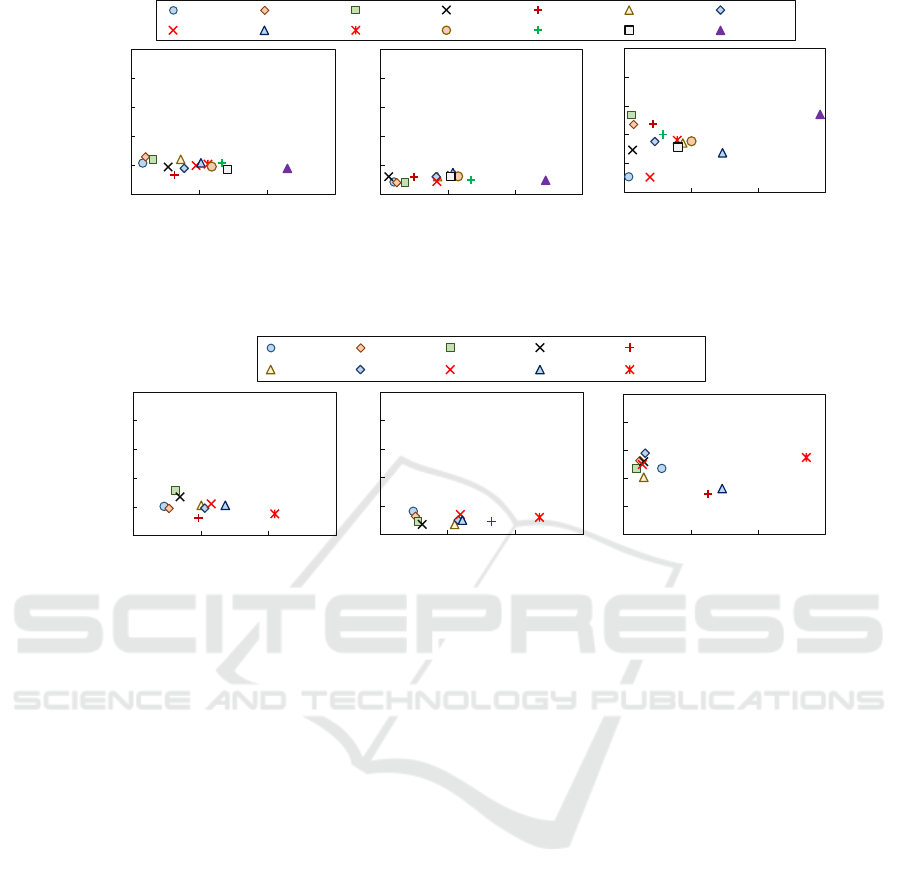
Training DataSet: For the training phase, we se-

lected fourteen workloads with different characteris-

tics of L3 cache miss ratio and average number of in-

structions per cycle (IPC), as shown in Fig. 2: Three

applications from the Rodinia Benchmark Suite (Che

et al., 2009): hotspot (HS), lower-upper decomposi-

tion (LUD), and streamcluster (SC). Five kernels and

pseudo-applications from the NAS Parallel Bench-

marks (Bailey et al., 1991): CG, FT, LU, SP, and

UA. Three applications from various other domains:

the Jacobi method (JA), the Poisson equation solver

(PO), and the STREAM benchmark (ST). Three ap-

plications from the Parboil Benchmark Suite (Stratton

et al., 2012): MRI, SPMV, and TPACF.

Validation DataSet: To validate SmartNodeTuner,

we selected ten applications that exhibit varying char-

acteristics in terms of CPU and memory usage, as de-

tailed in Fig. 3: Four from the Parboil Benchmark

suite: BFS, CUTCP, LBM, and SGEMM. Three from

the NAS Parallel Benchmark suite: BT, EP, and MG.

Three from other domains: FFT, HPCG, and NB. The

applications can also be categorized based on their de-

gree of parallelism, as measured using AMD uProf.

Low parallelism: limited scalability due to inherent

constraints in their computational structure or work-

load distribution, and include BFS, FFT, HPCG, NB,

and SGEMM. Medium parallelism: moderate scala-

bility, leveraging parallel resources more effectively

than low-parallelism workloads but not fully exploit-

ing the available threads. Examples are LBM and

MG-NAS. High parallelism: These applications efﬁ-

ciently scale across multiple threads, fully utilizing

the parallel capabilities of the hardware. Examples

include BT-NAS and CUTCP.

We have chosen these applications because of

their diversity in computational and memory access

patterns, which mirror real-world parallel cloud work-

loads. The training dataset includes applications with

varied L3 cache miss ratios and IPC, such as those

from the Rodinia and NAS-PB suites, enabling the

evaluation of our proposed framework under different

hardware utilization scenarios. Similarly, the valida-

tion dataset includes applications with distinct CPU

and memory usage behaviors, ranging from compute-

bound tasks like LBM to memory-intensive applica-

tions like HPCG, ensuring comprehensive coverage

of cloud-speciﬁc challenges such as resource alloca-

tion and heterogeneity.

CLOSER 2025 - 15th International Conference on Cloud Computing and Services Science

a) AMD-16 b) AMD-24 c) AMD-64

0.0

0.2

0.4

0.6

0.8

1.0

0 1 2 3

L3 Cache Misses

Average IPC

0.0

0.2

0.4

0.6

0.8

1.0

0 1 2 3

Average IPC

0.0

0.2

0.4

0.6

0.8

1.0

0 1 2 3

Average IPC

ST MRI JA TPACF CG-NAS UA-NAS SP-NAS

SC HS LU-NAS SPMV FT-NAS LUD PO

Figure 2: Behavior of each workload used to train the model employed by SmartNodeTuner.

0.0

0.2

0.4

0.6

0.8

1.0

0 1 2 3

L3 Cache Misses

Average IPC

0.0

0.2

0.4

0.6

0.8

1.0

0 1 2 3

Average IPC

0.0

0.2

0.4

0.6

0.8

1.0

0 1 2 3

Average IPC

EP-NAS FFT HPCG MG-NAS SGEMM

BFS NB BT-NAS CUTCP LBM

a) AMD-16 b) AMD-24 c) AMD-64

Figure 3: Behavior of each workload used to validate SmartNodeTuner.

5 EXPERIMENTAL EVALUATION

In this section, we discuss the results of employing

SmartNodeTuner to execute parallel workloads on a

private heterogeneous cloud. To assess the effective-

ness of our approach, we compared its results against

distinct scenarios:

STD-WN16, STD-WN24, and STD-WN64:

each workload was executed on the respective worker

node with the number of threads that matches the

number of cores (e.g., 16, 24, and 64, respectively),

which is the standard practice employed to execute

parallel workloads. Best-WN16, Best-WN24, and

Best-WN64: In this scenario, we conducted a thor-

ough search to determine the optimal number of

threads that achieved the best EDP for each node.

Each conﬁguration represents the execution of the

workload using the optimal number of threads on

each worker node. Random: a method where the

workloads are randomly assigned to worker nodes.

Kube-Scheduler: This scenario uses Kubernetes’

built-in scheduling component. Best-All: an ideal

scenario where each application was executed with

the best possible conﬁguration regarding worker node

selection and thread count, resulting in the lowest

energy-delay product. This optimal conﬁguration was

identiﬁed by exhaustively testing all combinations of

worker nodes, and thread counts for each workload.

5.1 Accuracy of SmartNodeTuner

Table 1 compares the conﬁgurations predicted by

SmartNodeTuner with those identiﬁed through ex-

haustive search (referred to as Best-All) for the ten

validation workloads. Each conﬁguration is repre-

sented as < worker node − #threads >. The table

also indicates the rank of SmartNodeTuner’s predic-

tion among all possible conﬁgurations. As shown,

no single conﬁguration (working node and number

of threads) provides the best trade-off between per-

formance and energy consumption across all applica-

tions. For instance, the optimal conﬁguration found

by Best-All for BFS is to run it with four threads

on the WN16 system, whereas the CUTCP bench-

mark performs best with 56 threads on the working

node with 64 cores. To further analyze this behav-

Energy-Aware Node Selection for Cloud-Based Parallel Workloads with Machine Learning and Infrastructure as Code

0.1

100

2 8 14 20 26 32 38 44 50 56 62

Energy-Delay Product

(x10³)

Number of Cores

SmartNodeTuner

Best-All

100

1000

10000

2 8 14 20 26 32 38 44 50 56 62

Number of Cores

SmartNodeTuner

Best-All

100

1000

10000

2 8 14 20 26 32 38 44 50 56 62

Number of Cores

WN16

WN24

WN64

Best-All

SmartNodeTuner

a) CUTCP b) FFT c) LBM

Figure 4: EDP behavior of three workloads when running on the evaluated platforms.

Table 1: Combinations found by Best-All and SmartNode-

Tuner for each workload.

Best-All

SmartNode

Tuner

Top-Best

(%)

EDP

Diff

BFS WN16-4 WN16-6 < 2% 2.05

BT-NAS WN64-52 WN64-64 < 8% 1.25

CUTCP WN64-56 WN64-56 < 1% 1.00

EP-NAS WN16-16 WN16-16 < 1% 1.00

FFT WN16-8 WN16-6 < 2% 1.01

HPCG WN16-8 WN16-8 < 1% 1.00

LBM WN24-12 WN16-14 < 7% 1.31

MG-NAS WN24-12 WN24-12 < 1% 1.00

NB WN16-4 WN16-2 < 2% 1.77

SGEMM WN16-8 WN16-8 < 1% 1.00

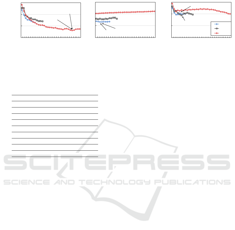
ior, Figure 4 illustrates the EDP for all evaluated con-

ﬁgurations of working nodes and thread counts when

running three applications with distinct characteris-

tics (CUTCP, FFT, and LBM). We also highlight the

conﬁgurations found by Best-All and predicted by

SmartNodeTuner.

For applications with a high average IPC and a

low ratio of time spent accessing main memory (in-

dicated by fewer L3 cache misses), the competition

for shared resources is reduced. In such cases, run-

ning these applications on a working node with more

cores results in signiﬁcant EDP reductions during ex-

ecution. This behavior is evident in the CUTCP ap-

plication, as shown in Figure 4.a, where the applica-

tion scales well and beneﬁts from the large number

of cores and cache memory available on the WN64

system. A similar pattern was observed for BT-NAS.

Conversely, for applications with limited paral-

lelism and a moderate ratio of time spent accessing

main memory, the best EDP results are achieved by

running them on a working node with fewer cores,

minimizing the impact of data communication among

threads. This was the case for applications such as

BFS, EP-NAS, FFT, HPCG, NB, and SGEMM. For in-

stance, Figure 4.b illustrates the scenario for the FFT

application, where the WN16 system delivered the

best results. Additionally, applications with a moder-

ate degree of TLP achieved optimal performance on

the working node with 24 cores, as observed in the

LBM application shown in Figure 4.c.

Analyzing the results obtained by SmartNode-

Tuner in Table 1, it correctly predicted the optimal

conﬁguration in half of the cases. While this accu-

racy rate may appear low, it underscores the complex-

ity of the optimization challenge, with 104 possible

conﬁgurations per workload. On top of that, 80% of

its predictions were within the Top-2 conﬁgurations,

and all were within the Top-8. Table 1 also com-

pares the EDP between SmartNodeTuner and Best-

All (EDP Diff column), with values normalized to the

Best-All results. Hence, a value close to 1.0 means

that SmartNodeTuner reaches a conﬁguration near the

optimal. In almost all cases, SmartNodeTuner pre-

dicted the combination of worker node and number

of threads within the 2% of best solutions, leading

to a difference of only 19% of EDP across all work-

loads. The worst case for SmartNodeTuner was for

the NB and BFS workloads due to the sensitivity of

these applications to thread synchronization issues.

For this type of application, increasing the number of

active threads leads to more time spent synchronizing

data within parallel regions, which can degrade per-

formance and energy efﬁciency.

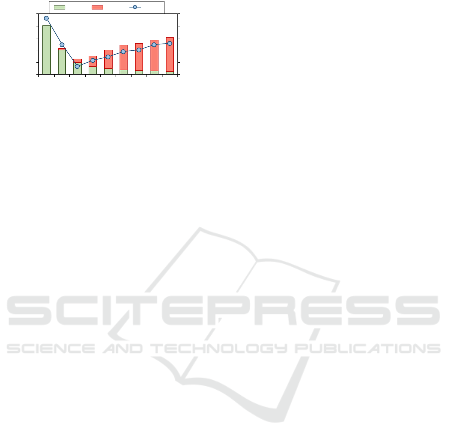
This behavior is illustrated for the BFS applica-

tion in Figure 5 on the working node with 16 cores

(WN16). The x-axis represents the number of ac-

tive threads. At the same time, the execution time

is divided into two parts: the time spent executing

the parallel region and the time spent synchronizing

data. Therefore, the total execution time is the sum

of these parts. The secondary y-axis shows the to-

tal energy consumption, measured in Joules. As de-

picted, the execution time decreases as the number

of threads increases from one to four. However, be-

yond this point, synchronization overhead surpasses

the execution time of the beneﬁts obtained due to par-

allelization, resulting in increased execution time and

energy consumption, thereby worsening the EDP. Al-

though SmartNodeTuner was able to predict a near-

optimal conﬁguration (WN16-6 instead of WN16-4),

the EDP difference compared to the Best-All solution

CLOSER 2025 - 15th International Conference on Cloud Computing and Services Science

100

200

300

400

500

0.0

2.0

4.0

6.0

8.0

10.0

1 2 4 6 8 10 12 14 16

Energy (Joules)

Execution Time (s)

Number of Cores

Parallel Critical Energy

Figure 5: Thread Scalability of BFS on the WN16.

was 2.05 times.

5.2 EDP Comparison

In this subsection, we compare the EDP results of

each strategy running the workloads on the target pri-

vate cluster, as described in Section 4. For that, Fig. 6

illustrates the EDP of each strategy normalized to the

Best-All for each workload, represented by the black

line. Moreover, Fig. 7 depicts the distribution of the

EDP results normalized to the best EDP achieved on

each workload (Best-All). Hence, the closer the val-

ues are to 1.0, the better the EDP. In this analysis, our

primary interest is achieving a distribution of EDP re-

sults on the validation workloads as close as possible

to the Best-All. Hence, an ideal outcome would be a

compact boxplot in Fig. 7, indicating low variability

in achieving the best EDP for each workload and near

1.0.

We begin by analyzing the EDP of our strat-

egy, SmartNodeTuner, compared to the standard ex-

ecution strategy on each worker node (STD-WN16,

STD-WN24, and STD-WN64). As shown in Fig. 6,

SmartNodeTuner achieved better EDP across most

cases. The most signiﬁcant gains by choosing an ideal

worker node and TLP degree were observed in ap-

plications with limited thread scalability due to data

synchronization overhead, such as NB and BFS. As

discussed by Suleman et al., (Suleman et al., 2008;

Lorenzon et al., 2018; Maas et al., 2024), using the

maximum number of threads to execute this kind of

workload increases execution time and energy usage

due to the overhead on the critical regions, nega-

tively impacting EDP. On the other hand, in scenarios

where ideal EDP aligns with maximum thread count,

the results were similar (e.g., EP-NAS for the STD-

WN16. Overall, SmartNodeTuner achieved EDP im-

provements, with geometric means showing enhance-

ments of 54.9%, 77.8%, and 81.7% on STD-WN16,

STD-WN24, and STD-WN64 conﬁgurations, respec-

tively. Even when compared to the best EDP achieved

per worker node (Best-WN16, Best-WN24, and Best-

WN64), SmartNodeTune achieves better overall EDP,

highlighting the importance of selecting not only the

optimal thread count per worker node but also ﬁnding

an ideal worker node to execute the given workload.

On average, across all workloads, SmartNodeTuner

improves EDP by 17.9%, 35.1%, and 43.4% over the

best threading conﬁguration on the machines, respec-

tively.

While Random and Kube-Scheduler can deliver

better EDP results than the standard execution on each

worker node, neither outperforms the EDP improve-

ments provided by SmartNodeTuner. On average,

SmartNodeTuner achieves a 38.2% higher EDP efﬁ-

ciency than Kube-Scheduler across all applications.

The main reason we found during the experiments is

that the decisions made by the scheduler do not con-

sider the efﬁciency in resource utilization, leading to

less optimal choices for node and thread allocation.

Instead, it considers resource availability, e.g., CPU

and memory behavior. Differently, SmartNodeTuner

considers the workload characteristics regarding re-

source efﬁciency when deploying it for execution, op-

timizing thread distribution, and node allocation.

Finally, let us consider the EDP distribution across

conﬁgurations, shown in Fig. 7. The goal here is

to achieve a compact distribution near 1.0, indicating

both low variability and a high EDP efﬁciency rel-

ative to the exhaustive search results (Best-All). In

this context, SmartNodeTuner maintained a consis-

tently narrow distribution, centered close to 1.0 across

various workloads. By contrast, the other conﬁgura-

tions have wider spreads and higher median values,

reﬂecting more signiﬁcant inconsistency and gener-

ally worse EDP efﬁciency overall.

5.3 Impact on the Performance and

Energy Consumption

Improving, at the same time, the energy efﬁciency

and performance in cloud computing environments is

challenging as it requires balancing both metrics so

that one metric is not compromised due to the im-

provements on the other. In this scenario, to assess

the efﬁcacy of SmartNodeTuner in achieving this bal-

ance, we compared the performance and energy con-

sumption to all the previously discussed strategies.

For that, Fig. 8a shows the performance reached

by each strategy normalized to the Best-All conﬁgu-

ration, considering the geometric mean of all work-

loads. In this plot, the closer the value is to 1.0, the

better the performance. Similarly, Fig. 8b depicts the

energy consumption normalized to the best result. In

this plot, the lower the value is, the less energy was

spent during execution.

Because our approach, SmartNodeTuner, can pre-

dict conﬁgurations that are most of the time within

Energy-Aware Node Selection for Cloud-Based Parallel Workloads with Machine Learning and Infrastructure as Code

0.0

0.2

0.4

0.6

0.8

1.0

1.2

EP-NAS FFT HPCG MG-NAS SGEMM BFS NB BT-NAS CUTCP LBM GMEAN

EDP Normalized

STD-WN16 WTD-WN24 STD-WN64 Best-WN16 Best-WN24 Best-WN64 KS Random SmartNodeTuner

Figure 6: EDP results on each workload, normalized to the Best-All, represented by the black line.

EDP Normalized to

Best-All

0.0

0.2

0.4

0.6

0.8

1.0

1.2

STD

WN16

STD

WN24

STD

WN64

Best

WN16

Best

WN24

Best

WN64

Kube

Sched

Random

SmartNodeTuner

Best

All

Figure 7: Distribution of EDP results for each strategy

across all workloads.

the Top-2%, it can reach energy consumption lev-

els as close to the ideal one (only 7.01% of differ-

ence) while not jeopardizing the overall performance

(10.5%) as the other strategies do. When compar-

ing SmartNodeTuner with the conﬁguration that de-

livers the lowest overall energy consumption (Best-

WN16), it is 5.3% more energy-hungry but reaches

performance levels 28.2% higher. When only the per-

formance matters, Best-WN24 can deliver better per-

formance without considering the Best-All conﬁgura-

tion (6% higher than SmartNodeTuner) at the price of

64.6% more energy spent.

5.4 Overhead of SmartNodeTuner

Achieving conﬁgurations consistently within the Top-

2% best solutions allows SmartNodeTuner to approx-

imate the EDP efﬁciency of an exhaustive search

(Best-All) with much lower overhead. Unlike exhaus-

tive search, SmartNodeTuner proﬁles each applica-

tion only once with a default conﬁguration, and the

inference process takes only 0.0093s per lookup. In

this scenario, the time it took for SmartNodeTuner to

run each target application with the standard conﬁg-

uration and predict an ideal combination of TLP de-

gree and worker node was only 413.75s, compared

to 26377.01s of the exhaustive search. On the other

hand, the feature extraction part for the ANN model

incurs the highest computational cost: 2.38 hours

on WN16, 2.79 hours on WN24, and 10.31 hours

on WN64, with respective energy costs of 3.42x10

J, 8.61x10

J, and 3.50x10

J. However, it is worth

mentioning that this extraction phase is performed

only once, and this cost can be further minimized via

strategies like sampling, reduced input sets, or dis-

tributed computing, which are not the goal of this pa-

per.

6 CONCLUSION

We have presented SmartNodeTuner, a framework

for optimizing the performance and energy consump-

tion when executing HPC workloads in cloud envi-

ronments using AI and IaC. It considers the behav-

ior of parallel workloads to predict ideal combina-

tions of worker nodes and TLP degrees. By incor-

porating IaC into the automation process of SmartN-

odeTuner, the resource management is simpliﬁed, be-

ing applied to diverse cloud infrastructures. When

evaluating SmartNodeTuner over the execution of ten

well-known parallel workloads on a heterogenous en-

vironment, we show that it predicts combinations that

reach EDP values close to the ones achieved by the

exhaustive search, improving the EDP by 38.2% com-

pared to the standard scheduler used by Kubernetes.

We also show that by employing SmartNodeTuner,

the application’s performance is marginally affected

while providing signiﬁcant energy savings. As fu-

ture work, we plan to increase the compatibility of

SmartNodeTuner with other cluster orchestrators, al-

lowing users more ﬂexibility in selecting cloud and

HPC solutions.

ACKNOWLEDGEMENTS

This study was partly ﬁnanced by the CAPES - Fi-

nance Code 001, FAPERGS - PqG 24/2551-0001388-

1, and CNPq.

CLOSER 2025 - 15th International Conference on Cloud Computing and Services Science

0.0

0.2

0.4

0.6

0.8

1.0

1.2

STD-WN16

WTD-WN24

STD-WN64

Best-WN16

Best-WN24

Best-WN64

Kube-Sched.

Random

SmartNodeTuner

Best-All

Perf. Normalized

(a) Performance

0.0

1.0

2.0

3.0

4.0

STD-WN16

WTD-WN24

STD-WN64

Best-WN16

Best-WN24

Best-WN64

Kube-Sched.

Random

SmartNodeTuner

Best-All

Energy normalized

(b) Energy consumption

Figure 8: Performance and Energy results for each strategy normalized to Best-All.

REFERENCES

Bailey, D. H., Barszcz, E., Barton, J. T., Browning, D. S.,

Carter, R. L., Dagum, L., Fatoohi, R. A., Frederick-

son, P. O., Lasinski, T. A., Schreiber, R. S., Simon,

H. D., Venkatakrishnan, V., and Weeratunga, S. K.

(1991). The nas parallel benchmarks and summary

and preliminary results. In ACM/IEEE SC, pages 158–

165, USA. ACM.

Barham, P., Dragovic, B., Fraser, K., Hand, S., Harris, T.,

Ho, A., Neugebauer, R., Pratt, I., and Warﬁeld, A.

(2003). Xen and the art of virtualization. SIGOPS

Oper. Syst. Rev., 37(5):164–177.

Borovits, N., Kumara, I., Krishnan, P., Palma, S. D.,

Di Nucci, D., Palomba, F., Tamburri, D. A., and

van den Heuvel, W.-J. (2020). Deepiac: deep

learning-based linguistic anti-pattern detection in iac.

In Proceedings of the 4th ACM SIGSOFT Interna-

tional Workshop on Machine-Learning Techniques

for Software-Quality Evaluation, MaLTeSQuE 2020,

page 7–12, New York, NY, USA. Association for

Computing Machinery.

Che, S., Boyer, M., Meng, J., Tarjan, D., Sheaffer, J. W.,

Lee, S.-H., and Skadron, K. (2009). Rodinia: A

benchmark suite for heterogeneous computing. In

IEEE Int. Symp. on Workload Characterization, pages

44–54, DC, USA. IEEE Computer Society.

Ham, T. J., Chelepalli, B. K., Xue, N., and Lee, B. C.

(2013). Disintegrated control for energy-efﬁcient and

heterogeneous memory systems. In IEEE HPCA,

pages 424–435.

Huang, H., Rao, J., Wu, S., Jin, H., Jiang, H., Che, H.,

and Wu, X. (2021). Towards exploiting cpu elas-

ticity via efﬁcient thread oversubscription. In Pro-

ceedings of the 30th International Symposium on

High-Performance Parallel and Distributed Comput-

ing, HPDC ’21, page 215–226, New York, NY, USA.

Association for Computing Machinery.

Kumara, I., Vasileiou, Z., Meditskos, G., Tamburri, D. A.,

Heuvel, W.-J. V. D., Karakostas, A., Vrochidis, S., and

Kompatsiaris, I. (2020). Towards semantic detection

of smells in cloud infrastructure code. ARXIV-CS.SE.

Lepiller, J., Piskac, R., Sch

af, M., and Santolucito, M.

(2021). Analyzing infrastructure as code to prevent

intra-update sniping vulnerabilities. International

Conference on Tools and Algorithms for the Construc-

tion and Analysis of Systems.

Liu, F., Tong, J., Mao, J., Bohn, R., Messina, J., Badger, L.,

and Leaf, D. (2012). NIST Cloud Computing Refer-

ence Architecture: Recommendations of the National

Institute of Standards and Technology. CreateSpace

Independent Publishing Platform, USA.

Lorenzon, A. F. and Beck Filho, A. C. S. (2019). Parallel

computing hits the power wall: principles, challenges,

and a survey of solutions. Springer Nature.

Lorenzon, A. F., De Oliveira, C. C., Souza, J. D., and Beck,

A. C. S. (2018). Aurora: Seamless optimization of

openmp applications. IEEE transactions on parallel

and distributed systems, 30(5):1007–1021.

Maas, W., de Souza, P. S. S., Luizelli, M. C., Rossi,

F. D., Navaux, P. O. A., and Lorenzon, A. F. (2024).

An ann-guided multi-objective framework for power-

performance balancing in hpc systems. In Proceed-

ings of the 21st ACM International Conference on

Computing Frontiers, CF ’24, page 138–146, New

York, NY, USA. Association for Computing Machin-

ery.

arquez, G., Villegas, M. M., and Astudillo, H. (2018).

A pattern language for scalable microservices-based

systems. In ECSA, NY, USA. ACM.

Masanet, E., Shehabi, A., Lei, N., Smith, S., and Koomey,

J. (2020). Recalibrating global data center energy-use

estimates. Science, 367(6481):984–986.

Navaux, P. O. A., Lorenzon, A. F., and da Silva Serpa, M.

(2023). Challenges in high-performance computing.

Journal of the Brazilian Computer Society, 29(1):51–

62.

Palma, S. D., Nucci, D. D., and Tamburri, D. A. (2020).

Ansiblemetrics: A python library for measuring

infrastructure-as-code blueprints in ansible. SOFT-

WAREX.

Saavedra, N. and Ferreira, J. F. (2022). Glitch: Automated

polyglot security smell detection in infrastructure as

code. ARXIV-CS.CR.

Sandobalin, J., Insfr

an, E., and Abrah

ao, S. M. (2017). An

infrastructure modelling tool for cloud provisioning.

IEEE International Conference on Services Comput-

ing (SCC).

Sandobal

ın, J., Insfran, E., and Abrah

ao, S. (2020). On the

Energy-Aware Node Selection for Cloud-Based Parallel Workloads with Machine Learning and Infrastructure as Code

effectiveness of tools to support infrastructure as code:

Model-driven versus code-centric. IEEE ACCESS.

Stratton, J., Rodrigues, C., Sung, I., Obeid, N., Chang, L.,

Anssari, N., Liu, G., and Hwu, W. (2012). Parboil: A

revised benchmark suite for scientiﬁc and commercial

throughput computing. Center for Reliable and High-

Performance Computing.

Subramanian, L., Seshadri, V., Kim, Y., Jaiyen, B., and

Mutlu, O. (2013). MISE: Providing performance

predictability and improving fairness in shared main

memory systems. In IEEE HPCA, pages 639–650.

Suleman, M. A., Qureshi, M. K., and Patt, Y. N.

(2008). Feedback-driven threading: Power-efﬁcient

and high-performance execution of multi-threaded

workloads on cmps. SIGARCH Comput. Archit. News,

36(1):277–286.

Vuppalapati, C., Ilapakurti, A., Chillara, K., Kedari, S., and

Mamidi, V. (2020). Automating tiny ml intelligent

sensors devops using microsoft azure. IEEE Interna-

tional Conference on Big Data (Big Data).

CLOSER 2025 - 15th International Conference on Cloud Computing and Services Science