A Case Study on Defining Infrastructure Sensor Positions with

Consideration of Existing Infrastructure

Philipp Klein

Institute of Vehicle Concepts, German Aerospace Center, Pfaffenwaldring38-40, 70569 Stuttgart, Germany

Keywords: Intelligent Traffic Systems, Infrastructure Sensors, GIS Analysis.

Abstract: Support by infrastructure sensors can be crucial to enable automated vehicles to safely navigate complex

urban driving environments. Finding the suitable positions for infrastructure sensors is a complex problem

with different demands and factors. This paper proposes a method of automating the process of selecting

positions for infrastructure sensors in a 2D environment. The positions are selected using available data of the

streets, for sensor placement suitable existing infrastructure and sensor coverage demands. This methodology

is then applied to finding sensor positions in the neighborhood of Lausitzer Platz in Berlin, Germany. The

sensor demands for this are to taken from a virtual roll out scenario of the U-Shift vehicle concept. This is

done by first finding suitable sensor positions for the bigger streets with the highest cargo and person

transportation demand and then covering of every street in the neighborhood. In this use case more than half

the sensor could be placed on existing infrastructure, if there is a high density of existing infrastructure that

is suitable for the placement of sensors.

1 INTRODUCTION

Although car manufacturers have made a lot progress

in increasing the capabilities of their driving

assistance systems in the recent years, eliminating the

need of constant human supervision remains an

unsolved challenge for production cars. This is

especially true for urban and suburban traffic. The

driving environment in these is highly complex with

a lot of other traffic participants, some of which are

Vulnerable Road Users (VRU) like for example

pedestrians and cyclist. Another big challenge in

these scenarios are occlusions of the field of view of

automated vehicles by other traffic participants,

buildings and other objects like trees and signs. One

approach to enable save navigation through this

complex urban traffic is the support by other

automated vehicles and infrastructure to provide

additional information. To exchange this information

between traffic participants ‘Vehicle to Everything’

communication is used. as standardized by the

European Telecommunications Standards Institute

(ETSI) as ITS-G5 (ETSI 2020). ETSI defines

messages over which perceived objects (CPM),

information about the ego vehicle (CAM) and

https://orcid.org/0009-0000-9343-1536

coordination of maneuvers and trajectories (MCM),

can be communicated with other traffic participants.

A way to achieve a higher quality of information

is the placement of sensors outside of vehicles. The

acquired information is then shared with traffic

participants via CPM messages.

Infrastructure sensor systems have an inherent

advantage by being placed higher than vehicles and

being able to have multiple perspectives of the

driving situation. The extent of this sensor coverage

can range from only on some points of interest, like

for example especially dangerous intersections, to

coverage of the whole area of operation, as proposed

in the concept Managed automated driving (MAD)

(Schindler 2023).

There are different coverage and economic,

demands on the infrastructure. To cover a area of

relevant size, many sensors have to be placed and a

lot of factors have to be considered to find suitable

positions. While there has been previous work on

improving and automating larger scale placement of

other traffic infrastructure like street lights (Baihaki

et al. 2024; Ishak 2021) or infrastructure

communication units (Huo et al. 2024). Work on the

placement of infrastructure sensors is usually focused

on finding an optimal sensor configuration, with the

582

Klein, P.

A Case Study on Deﬁning Infrastructure Sensor Positions with Consideration of Existing Infrastructure.

DOI: 10.5220/0013419800003941

Paper published under CC license (CC BY-NC-ND 4.0)

In Proceedings of the 11th International Conference on Vehicle Technology and Intelligent Transport Systems (VEHITS 2025), pages 582-587

ISBN: 978-989-758-745-0; ISSN: 2184-495X

least number of sensors possible (Akbarzadeh et al.

2014; Argany et al. 2018; Geissler and Grafe 2019).

In a real-world rollout however, the number of needed

sensors is not the only factor to consider. The cost of

constructing a pole, to place the sensor upon, can be

multiple times the cost of the actual sensor unit. This

paper proposes a methodology for finding a suitable

infrastructure sensor configuration for a quarter,

prioritizing existing infrastructure to place sensor

units. The approach uses a 2D representation of the

environment using geographic data in formats of the

Geographic information system (GIS). Chapter 2

describes the methodology of placing the sensors,

Chapter 3 then applies the methodology to the use

case of a virtual scenario of an operation of U-Shift

vehicles in the neighborhood of Lausitzer Platz in

Berlin, Germany.

2 METHODOLOGY

In this section the algorithm for finding sensor

positions is described. First the necessary input

parameters are described, then the actual placement

algorithm.

2.1 Input Parameters

The input parameters for the proposed automated

finding of infrastructure sensor positions are: street

data, sensor demands, candidate poles and loss

function.

The required street data contains all streets on

which sensors are to be placed. A street is defined as

a polynomial path between two intersection points.

This selection is based on spatial limits. Within these

spatial limits single streets can also be selected or

deselected based on preference.

There are two ways to define sensor demands. The

first are fixed-point demands and define a maximum

distance, within which an infrastructure sensor has to

be placed. This can used to make sure a point of

interest, like for example intersection points or bus

stops have sufficient sensor coverage. The second

way of defining a sensor demand is a sensor density

demand. It is defined by a maximum distance

between to sensor poles and can be varied for each

street. Through this the sensor density can be varied

to consider streets with higher risk of personal harm,

like for example streets with unprotected bicycle

paths or streets near schools.

In some cases, existing infrastructure like lamp

posts and traffic lights can be used to place sensors.

This avoids the cost and planning associated with the

construction of sensor poles in an urban environment.

The input candidate poles is a list of the positions of

all existing infrastructure suitable for placing sensors.

The fourth input parameter is the cost function. It

defines what cost the placement of a sensor and pole

has. This cost can be an economic cost, but also

societal costs like use of public space. The function

can contain per piece costs for sensors or poles but

also for example cost dependent on the location of the

pole.

2.2 Placement Algorithm

The algorithm starts by searching Sensor positions to

fulfil all fixed-point demands. The algorithm checks,

if there are any candidate poles that fulfil the

maximum distance demands. If that is the case, the

sensors are placed on that location. If there is no

suitable candidate pole, a new pole is placed directly

at the fixed-point demand.

Figure 1: Flowchart of the placement algorithm to meet

fixed-point demands.

In the next step the streets are separated into street

sections. A street section is defined as the area

between two fixed-point sensor poles. To find a

suitable sensor configuration, the following process is

done for each street section: In the first step, the

minimum number of poles required for covering the

street section are placed in a way, that the distances

between all sensor pole on the street section is the

same. This sensor configuration is then saved as

configuration 1 and the cost of is determined through

the cost function. In the next step the nearest pole

candidate for each optimal sensor positions it is

A Case Study on Deﬁning Infrastructure Sensor Positions with Consideration of Existing Infrastructure

583

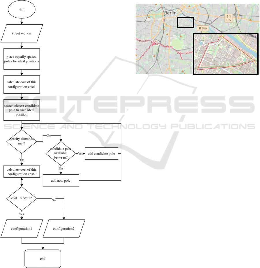
determined and then checked if the maximum

distance requirements are still fulfilled for all

distances between poles. If not, a candidate pole in

between is searched in between the two poles, which

don’t fulfil the requirement. If none is found, a new

pole is placed in the middle of these two poles. When

all distances between poles are below the maximum

distance, this sensor configuration is called sensor

configuration 2 and its cost is calculated. Then the

cost of both sensor configurations is compared and

the configuration with the lower cost is picked.

Figure 2: Flowchart of the placement algorithm to meet

density demands.

3 APPLICATION

In this chapter the proposed algorithm for finding a

suitable sensor configuration is applied to a specific

use case. The use case is a virtual scenario of an

operation of a fleet of U-Shift vehicles in the

neighborhood of Lausitzer Platz in Berlin. The

scenario and the parameters and data inputs derived

from it are specified in the following subchapter.

Then the results for a partial and a full coverage of the

streets with sensors are presented.

Figure 3: Definition of the Neighbourhood Lausitzer Platz.

3.1 Use Case and Input Parameters

The goal of the generated sensor configuration is the

support of a fleet of U-Shift vehicles in the

neighborhood of Lausitzer Platz in Berlin, Germany

in a virtual scenario. The neighborhood is defined as

the area marked in red in Figure 3 and covers around

1 square kilometer. The U-Shift vehicle concept is a

modular and driverless vehicle. The driving module

is separated from the transport capsule. This enables

the vehicle to fulfill different driving demands by

loading different capsules. Examples for this are a

Cargo Capsule for the delivery of goods and a Person

Capsule for transporting people.

The street data for the finding of sensors positions

is taken from data provided through the data portal

FIS-Broker(Stadt Berlin) by the city of Berlin. The

data is filtered to enable two coverage scenarios to be

investigated. In the first scenario, only the most

important streets in the neighborhood are covered

with sensors. For this scenario streets are selected by

the following criteria. Firstly, Streets with a high

density of shops and restaurants are picked to enable

U-Shift to services Cargo demands. Streets with a

high density of available candidate poles for sensor

placement are also preferred, since this could reduce

the cost of sensor placements. In the last step some

streets not fulfilling the previous requirements to

achieve a well-connected street network without any

VEHITS 2025 - 11th International Conference on Vehicle Technology and Intelligent Transport Systems

584

dead ends. The second scenario then covers all streets

in the neighborhood.

The list of candidate poles is created using FIS-

Broker data of traffic lights as well as street lights.

The street lights data contains categories for each

street light. These categories were then evaluated for

suitability for sensor placement using samples from

pictures in google street view. The results were used

to filter out street lamps unsuitable for sensor

placement.

The fixed-point demands on the infrastructure

sensors are the following: All intersection points are

set to have a maximum distance of 5 meters to the

next sensor pole to provide additional safety. In

addition to that all U-Shift Cargo and Person pick up

points are set to have a maximum distance off 5

meters to the next sensor pole. This demand is set to

assist the vehicles for the high precision backwards

driving and give more security to passengers entering

the person capsules.

To ensure safe operations of the U-Shift fleet, a

complete coverage of the area of operation by

infrastructure sensors is defined. The maximum

distance between sensors units was defined as 80m,

as proposed in the MAD feasibility study (Weimer

2020). For streets with bicycle lane a maximum

distance between sensors of 50m was chosen, to give

more safety to vulnerable road users.

For the cost function a cost of 1 unit or placing

sensors on existing infrastructure and 10 units for

placing a new sensor pole is chosen. The goal of this

is to represent the additional cost of construction for

a new pole. This results in the following cost function

𝑐𝑜𝑠𝑡



for a street section with the number of

newly placed poles 𝑛



and number of candidate

poles used ∗𝑛



𝑐𝑜𝑠𝑡



10∗𝑛



 1∗𝑛



(1)

3.2 Results Partial Coverage

As discussed, in the first scenario not all streets of the

neigborhood of Lausitzer Platz are considered for the

sensor configuration. The scenario contains 69 of the

97 total streets of the area. Figure 4 shows the

considered streets in black, cases where new sensor

posts would have to be placed in red and locations

were sensors could be placed on existing

infrastructure in blue.

The detailed distribution of the sensor position

can be seen in Table 1. 52 sensor units were placed

overall. For 133 of them existing infrastructure could

be used, 119 new poles were placed. To fulfill the

Whereas

fulfil

the

density

demands

85%

the

Figure 4: Infrastructure configuration to partly cover the

streets of Lausitzer Platz.

Table 1: Distribution of placed sensors for the partial rollout

scenario of Lausitzer Platz.

infrastructure

use

new poles

Intersection 8 46

Cargo 6 18

Person 3 35

densit

116 20

overall 133 119

fixed-point demands (intersection, cargo and person),

12% of the poles were existing infrastructure. sensors

were placed on existing infrastructure. This large

difference can be explained by the low maximum

distance parameters used for the fixed-point demands.

3.3 Results Full Coverage

The second scenario includes all 97 streets. The final

sensor configuration contains 342 sensor poles

overall. The streets and positions can be seen in

Figure 5, using the same colours as Figure 4. The

detailed distribution of the placed sensors can be seen

in Table 2. To fulfil the fixed-point demands, most

poles

had to be newly placed. 58% of the sensors to

fulfil density requirements could use existing

infrastructure.

Figure 5: Infrastructure configuration to cover all streets of

Lausitzer Platz.

A Case Study on Deﬁning Infrastructure Sensor Positions with Consideration of Existing Infrastructure

585

Table 2: Distribution of placed sensors for the full rollout

scenario of Lausitzer Platz.

infrastructure

used

new poles

Intersection

8 57

Cargo

6 25

Person

3 43

density

116 84

overall

133 209

Compared to the partial coverage scenario, all

additionally placed sensors were newly placed. Most

of these streets have historic gas-powered street

lights. These are specific to Berlin and because of

their low height not suitable for sensor placement.

This shows that the suitability of the existing

infrastructure for sensor placement can highly

influence the number of sensor poles that have to be

constructed and therefore the cost of covering an area

with infrastructure sensors.

4 CONCLUSION AND FUTURE

WORK

A method for automating the process of finding a

configuration of infrastructure sensors for a large area

was developed. It can fulfil both fixed-point and

density demands. It considers existing infrastructure

suitable for sensor placement and uses a cost function

to compare different sensor configurations. This

methodology was then applied to two virtual

coverage scenarios for a neighborhood in Berlin,

Germany. The first scenario covers only parts of the

streets and the second all streets. For the partial

coverage scenario around half the sensors could be

placed on existing infrastructure and it could be

shown, that the strictness of the sensor demands and

suitability of the existing infrastructure influences the

share of newly placed poles and therefore influence

the cost in a real-world rollout. However, the

methodology was only applied to one specific

neighborhood. To verify and generalize the results the

same methodology will have to be applied to more

locations with urban or suburban traffic.

Since the methodology is based on a 2D model of

the environment, it can’t consider possible obstacles

like trees, parking cars and buildings. Therefore, the

method provides a first overview of the sensor

placement and gives a starting point for cost

estimation and exact pole positioning. For a real-

world rollout however, every position will still have

to be verified to consider all the additional restrictions

in the real world or a highly accurately modelled 3D

environment.

The placement of sensors in a real-world rollout

can also have many cost factors and constraints not

considered by the proposed methodology. Examples

for that are the availability of electrical grid

connection and cost of providing internet connection

to the individual locations. To take this into account

an extension of the cost function or additional

constraints on sensor positions would be possible.

The biggest challenge for that, is the availability of

high-resolution data of these factors.

REFERENCES

Akbarzadeh, Vahab; Lévesque, Julien-Charles; Gagné,

Christian; Parizeau, Marc (2014): Efficient sensor

placement optimization using gradient descent and

probabilistic coverage. In Sensors (Basel, Switzerland)

14 (8), pp. 15525–15552. DOI: 10.3390/s140815525.

Argany, Meysam; Karimipour, Farid; Mafi, Fatemeh;

Afghantoloee, Ali (2018): Optimization of Wireless

Sensor Networks Deployment Based on Probabilistic

Sensing Models in a Complex Environment. In JSAN 7

(2), p. 20. DOI: 10.3390/jsan7020020.

Baihaki, Rifki Ilham; Mursyidah, Indah Lutfiyatul;

Darmaji, Darmaji (2024): Efficient Streetlight

Placement Using Dominating Set Theory. In CGANT

Journal of Mathematics and Applications 5 (1), pp. 19–

26. DOI: 10.25037/cgantjma.v5i1.113.

ETSI (2020): ETSI EN 302 663. ITS-G5 Access layer

specification for Intelligent Transport Systems

operating in the 5 GHz frequency band.

Geissler, Florian; Grafe, Ralf (2019): Optimized sensor

placement for dependable roadside infrastructures. In :

The 2019 IEEE Intelligent Transportation Systems

Conference - ITSC. Auckland, New Zealand, 27-30

October 2019. 2019 IEEE Intelligent Transportation

Systems Conference - ITSC. Auckland, New Zealand,

10/27/2019 - 10/30/2019. Institute of Electrical and

Electronics Engineers; IEEE Intelligent Transportation

Systems Society. Piscataway, NJ: IEEE, pp. 2408–

2413.

Huo, Yan; Yang, Ruixue; Jing, Guanlin; Wang, Xiaoxuan;

Mao, Jian (2024): A multi-objective Roadside Units

deployment strategy based on reliable coverage

analysis in Internet of Vehicles. In Ad Hoc Networks

164, p. 103630. DOI: 10.1016/j.adhoc.2024.103630.

Ishak, Zulkifli (2021): Placement accuracy algorithm for

smart street lights. In Turkish J. Electr. Eng. Comput.

Sci. 29.2, pp. 845–859.

Schindler, Julian (2023): Managed Automated Driving

(MAD) - A Concept for Empowering Road

Infrastructure.

Stadt Berlin: FIS-Broker. Edited by Stadt Berlin. Available

online at https://fbinter.stadt-berlin.de/fb/index.jsp.

VEHITS 2025 - 11th International Conference on Vehicle Technology and Intelligent Transport Systems

586

Weimer, Jürgen (2020): U-Shift MAD Managed

Automated Driving für U-Shift. Machbarkeitsstudie

Zulassungsfähigkeit und Wirtschaftlichkeit. With

assistance of Miriam Grünhäuser, Alexander Wiemer,

Anne Brunßen, Marc Zofka, Tobias Fleck, Marcus

Conzelman et al.

A Case Study on Deﬁning Infrastructure Sensor Positions with Consideration of Existing Infrastructure

587