L2C: Learn to Clean Time Series Data

Mayuresh Hooli

and Rabi Mahapatra

Texas A&M University, College Station, U.S.A.

{mayurhooli, rabi}@tamu.edu

Keywords:

Data Cleaning, Machine Learning, Time Series Analysis, Outlier Detection, Data Imputation, Internet of

Things (IoT), Support Vector Regression (SVR).

Abstract:

In today’s data-driven economy, where decisions hinge on vast amounts of data from diverse sources such as

social media and government agencies, the accuracy of this data is paramount. However, data complexities

including errors from missing information and outliers challenge its integrity. To address this, we introduce a

novel machine learning framework, L2C (Learn to Clean), speciﬁcally designed to enhance the cleanliness of

time series data. Unlike existing methods like SVR and ARIMA that are limited to handling one or two types

of outliers, L2C integrates techniques from SVR, ARIMA, and Loess to robustly identify and correct for all

three major types of outliers—global, contextual, and collective. This paper marks the ﬁrst implementation of

a framework capable of detecting collective outliers in time series data. We demonstrate L2C’s effectiveness

by applying it to air quality sensor data sampled every 120 seconds from wireless sensors, showcasing superior

performance in outlier detection and data integrity enhancement compared to traditional methods like ARIMA

and Loess.

1 INTRODUCTION

L2C, or ‘Learn to Clean,’ revolutionizes time series

data integrity by using advanced machine learning

techniques like SVR (Muller et al., 1999), ARIMA

(Box and Jenkins, 1976), and Loess (Deng et al.,

2005) to handle global, contextual, and collective out-

liers. This framework operates on both edge devices

and the cloud, processing data streams from sources

such as air quality sensors at 120-second intervals.

The use of serverless analytics platforms, particularly

in edge computing, signiﬁcantly reduces the compu-

tational burden when managing large datasets across

distributed networks (Nastic and Rausch, 2017). By

improving data reliability at the source, L2C enables

cleaner, more accurate datasets, supporting informed

decision-making in today’s data-driven economy.

Figure 1: Stages of the Machine Learning Process: Data is

cleaned and prepared for analytics, the model is trained on

this data, and then tested for potential improvements.

https://orcid.org/0000-0003-4938-3447

1.1 Types of Challenges for Data

Cleaning

In this research, we address two principal challenges

in data cleaning: NULL values and outliers. While

NULL values are straightforward to identify as miss-

ing or blank entries, outliers are more complex and

can be categorized into three distinct types:

1. Global Outliers: Data points that deviate signiﬁ-

cantly from the majority of the dataset. These can

be identiﬁed through visual analysis and are dis-

tant from other observations. They can often be

removed with minimal computational effort.

2. Contextual Outliers: Data points that appear

anomalous only within a speciﬁc context. In time-

series data, for example, a value might be con-

sidered normal in one period but an outlier in an-

other. These outliers depend heavily on temporal

or other contextual factors.

3. Collective Outliers: Groups of data points that,

while individually normal, collectively deviate

from expected patterns. These do not conform to

the typical classiﬁcation of global or contextual

outliers but can still disrupt data analysis due to

their group behavior.

Each type of outlier presents unique challenges

Hooli, M. and Mahapatra, R.

L2C: Learn to Clean Time Series Data.

DOI: 10.5220/0013421300003944

Paper published under CC license (CC BY-NC-ND 4.0)

In Proceedings of the 10th International Conference on Internet of Things, Big Data and Security (IoTBDS 2025), pages 361-369

ISBN: 978-989-758-750-4; ISSN: 2184-4976

361

for identiﬁcation and remediation, demonstrating the

intricacies involved in cleaning data beyond simple

NULL value handling.

1.2 Current Techniques

Several established techniques are widely used for

outlier removal in data cleaning. These methods are

designed to detect and handle different aspects of

anomaly detection:

• Interquartile Range (IQR): This method uses

the interquartile range, the difference between the

25th percentile (Q1) and the 75th percentile (Q3).

Outliers are deﬁned as data points falling below

Q1 − 1.5 × IQR or above Q3 + 1.5 × IQR.

• ARIMA: A time-series forecasting model that

identiﬁes outliers by detecting deviations from

expected trends. However, it has limitations in

real-time processing due to its high computational

costs.

• Loess: A non-parametric method that ﬁts multi-

ple regressions in localized regions of the data. It

is highly effective for detecting outliers in scatter-

plot data by identifying points that deviate from

predicted trends based on local smoothing.

1.3 Motivation and Contribution: L2C

Despite the effectiveness of these established tech-

niques in handling global and contextual outliers indi-

vidually, they lack the capability to manage both types

simultaneously and fall short in effectively addressing

collective outliers (Aggarwal, 2015). Furthermore,

existing methods offer no comprehensive solution for

imputing NULL values, exposing a signiﬁcant gap in

current data cleaning approaches. These limitations

become particularly problematic in large-scale IoT

datasets, where traditional models like ARIMA are

inefﬁcient for real-time processing due to their high

computational demands (Salman and Jain, 2019).

To bridge this gap, we have developed Learn to

Clean (L2C), a machine learning-based solution de-

signed to handle real-time data streams in IoT envi-

ronments. L2C addresses the limitations of existing

methods by providing a comprehensive data clean-

ing framework capable of managing global, contex-

tual, and collective outliers, as well as NULL values.

Our approach integrates advanced techniques such as

ARIMA, Loess, and Interquartile Relationships, en-

suring the system can adapt to various types of out-

liers.

In addition, Support Vector Regression (SVR) is

incorporated to enhance L2C’s ability to handle non-

linear data, signiﬁcantly improving its performance

in time-series predictions (Muller et al., 1999). De-

signed for use in edge computing environments, L2C

processes real-time data streams with reduced latency,

improving both efﬁciency and accuracy (Nastic and

Rausch, 2017). By automating the detection and re-

moval of outliers, as well as the imputation of NULL

values, L2C sets new standards for accuracy and scal-

ability in data preprocessing, making it particularly

well-suited for large-scale IoT applications.

Our work on L2C has contributed to the ﬁeld by

offering a scalable, real-time data cleaning solution

that addresses challenges previously unmet by exist-

ing methods. Through L2C, we have advanced the

capability of data cleaning systems to efﬁciently pro-

cess complex, high-volume datasets in real-world IoT

environments.

2 PROCEDURE FOR L2C

This research focuses on two types of errors in edge

device datasets: outliers and NULL values. Outliers

are categorized into three types: Global, Contextual,

and Collective (Aggarwal, 2015). While NULL val-

ues are straightforward to identify and handle, detect-

ing outliers requires more sophisticated techniques.

Standard algorithms such as Loess and Ensemble-

SVR are effective in managing common outliers but

struggle with complex cases (Deng et al., 2005), espe-

cially Collective outliers, which some methods even

suggest cannot be fully removed (Aggarwal, 2015).

To address these challenges, we propose a multi-

step hybrid approach that combines machine learning

models like SVR with time-series analysis. This ap-

proach is designed to handle all three types of out-

liers while also imputing missing values, enhancing

the overall accuracy of data cleaning in large IoT

datasets (Mahdavinejad et al., 2018). The integra-

tion of serverless real-time data analytics platforms

for edge computing ensures that our process is efﬁ-

cient and scalable (Nastic and Rausch, 2017), making

it suitable for high-volume data environments where

timely and accurate data processing is critical.

2.1 Step-1: Initial Outlier Removal

In the ﬁrst phase of outlier treatment, easily identiﬁ-

able outliers are removed using two techniques: In-

terquartile Range (IQR) and Support Vector Regres-

sion (SVR). The IQR rule provides a quick and ef-

fective method for detecting global outliers, deﬁned

using the following calculations:

IoTBDS 2025 - 10th International Conference on Internet of Things, Big Data and Security

362

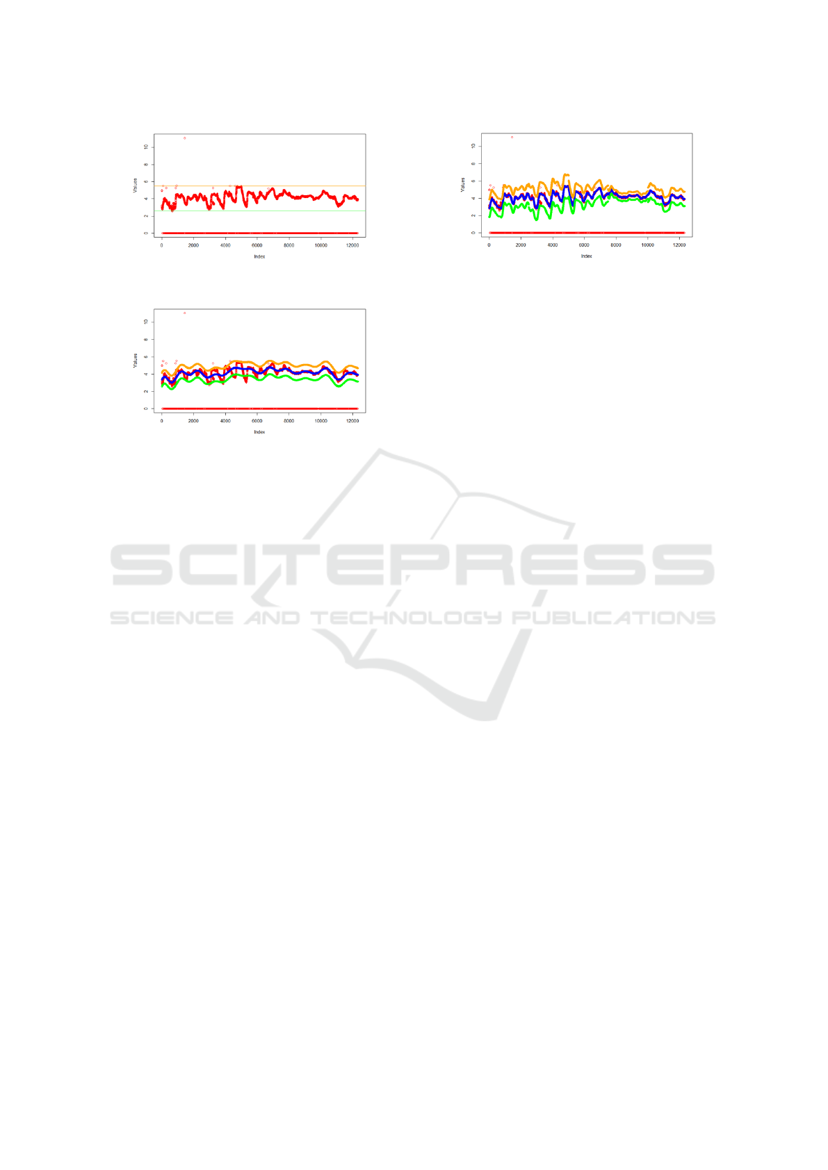
Figure 2: Data cleaned using the IQR rule. Contextual and

collective outliers remain.

Figure 3: Data cleaned using SVR. Some valid points are

removed along with outliers, but a more accurate ﬁt would

increase computational cost.

U pper = Q3 + 1.5 × IQR

Lower = Q1 − 1.5 × IQR

(1)

Where:

IQR = Q3 − Q1 (2)

Global outliers outside the Upper and Lower

bounds are removed, as illustrated in Figure 19.

While this method is efﬁcient, it has limited impact

on contextual and collective outliers.

To handle non-linearities in time series data, we

apply SVR, which provides a more accurate method

for outlier detection. Although SVR is computation-

ally more intensive, it accommodates non-linear pat-

terns, improving the outlier detection process. We de-

ﬁne a range for acceptable points using the standard

deviation of predictions, calculated as follows:

Top = Predicted + α

Bottom = Predicted − α

(3)

While SVR improves the precision of outlier de-

tection, it may remove some valid data points. In-

creasing the ﬁt accuracy would require more process-

ing time, which limits its real-time application.

2.2 Step-2: SVR

Support Vector Regression (SVR) is a robust non-

linear technique, but its computational complexity,

O(n

), makes it time-consuming, particularly for

Figure 4: Cleaned data after outlier removal using s-SVR,

with the dataset divided into 5 parts. Most outliers, includ-

ing contextual ones, are removed, while non-outlier data

points remain intact. The split predictions for upper (or-

ange) and lower (green) bounds are visible.

large datasets with high variability. While parame-

ter tuning can improve accuracy, it further increases

computation time.

To mitigate this, we introduce split-SVR (s-SVR),

which divides the dataset into smaller subsets, applies

SVR to each subset, and merges the results. This ap-

proach adds a tolerance margin, making it more suit-

able for real-time dynamic environments. The pro-

cess involves data splitting, ﬁltering with tolerance,

and merging, though it is not yet fully automated.

To account for variability in predictions, we calcu-

late the standard deviation of SVR-predicted values,

deﬁning upper and lower bounds as follows:

Top = Predicted + (α of SVR) (4)

Bottom = Predicted − (α of SVR) (5)

These bounds allow for the removal of global out-

liers and assist in identifying contextual outliers. With

s-SVR, users have less concern over hyperparameter

tuning, as the tolerance adjustment simpliﬁes the out-

lier removal process. Although the SVR curves do

not perfectly ﬁt the data, they are sufﬁcient to remove

most outliers, including contextual ones.

2.3 Step-3: Split Data into Subsets

While SVR and s-SVR remove most outliers, there is

a risk of eliminating valid data if not properly tuned.

To mitigate this, we proceed with a combination of

IQR and s-SVR, which retains more data. However,

both techniques struggle with certain contextual and

collective outliers, which can still affect predictions.

To address these remaining outliers, we introduce

a new step combining time series analysis with regres-

sion, ensuring alignment with previous steps. This

approach applies similarly after either IQR or s-SVR,

and we test it using IQR for broader outlier coverage.

Given the non-linear nature of the data, we sep-

arate trends using the ﬁrst difference to identify the

L2C: Learn to Clean Time Series Data

363

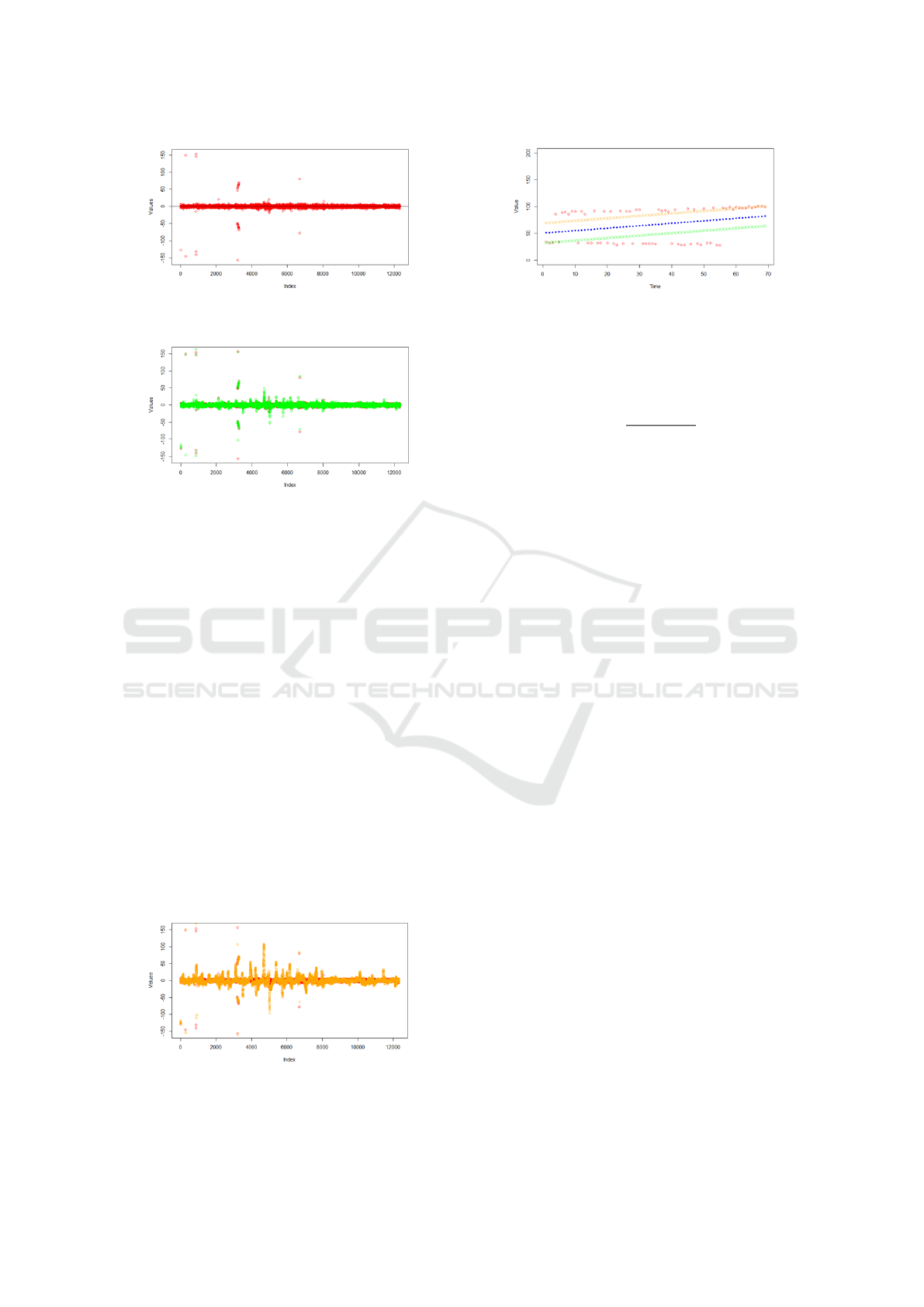
Figure 5: First difference between consecutive points show-

ing the rate of change in the data.

Figure 6: Data when the ﬁrst difference is calculated at a

frequency of 5. The variation is manageable for further

analysis.

underlying patterns. Through trial and error, a fre-

quency of 5 was found to be ideal for identifying

trends, though adjustments are needed for the ﬁrst few

points. The trend values are calculated as follows:

= a

− a

= a

− a

= a

− a

= a

− a

= a

− a

= a

− a

n−1

= a

− a

n−5

While trends are identiﬁable, not all trends are

equally informative due to the varying number of data

points in each trend. To ensure effective outlier de-

tection, the data is split into subsets based on trend

Figure 7: Data when the ﬁrst difference is calculated at a

frequency of 25. The variation is signiﬁcantly higher com-

pared to a frequency of 5.

Figure 8: Linear Regression for Phase-2: Outlier removal

after trend separation. The linear model poorly ﬁts the data,

leaving many outliers within the deﬁned parameters.

changes. We calculate the ﬁrst difference and check

for sign changes using:

p+1

× b

p+1

× b

(6)

If c

is 0 or 1, the trend remains constant, but if

= −1, it indicates a trend shift. We create new

subsets at each point where c

= −1.

For practical application, we require each subset

to contain at least 5 data points. If fewer than 5 points

exist, the subset is combined with adjacent subsets to

maintain a consistent trend. This ensures that each

subset has sufﬁcient data for further outlier analysis.

2.4 Step-4: Non-Linear Outlier

Detection and Removal

After separating trends, we now test multiple datasets

for contextual and collective outliers. Linear regres-

sion is initially applied but fails to effectively remove

outliers, particularly at the beginning of the dataset

(see Figure 8). Given the non-linear nature of the data,

a non-linear approach is necessary for further outlier

detection.

Given its success in earlier phases, we apply Sup-

port Vector Regression (SVR) to handle the non-

linearity. However, in this test, SVR overﬁts the data

by attempting to include all points, as shown in Fig-

ure 9. While SVR is useful for detecting contextual

outliers, it struggles with collective outliers due to its

tendency to ﬁt all data points together, making it difﬁ-

cult to distinguish between valid and anomalous data.

To mitigate overﬁtting, we implement Loess (Lo-

cal Regression), a non-linear technique that avoids the

pitfalls of SVR overﬁtting. Loess provides a more

balanced approach, as illustrated in Figure 10, effec-

tively removing outliers while preserving the overall

trend in the data.

Despite the success of Loess in removing outliers,

the process increases the number of NULL values in

the dataset, necessitating imputation. Standard impu-

tation techniques, such as replacing with the mean or

IoTBDS 2025 - 10th International Conference on Internet of Things, Big Data and Security

364

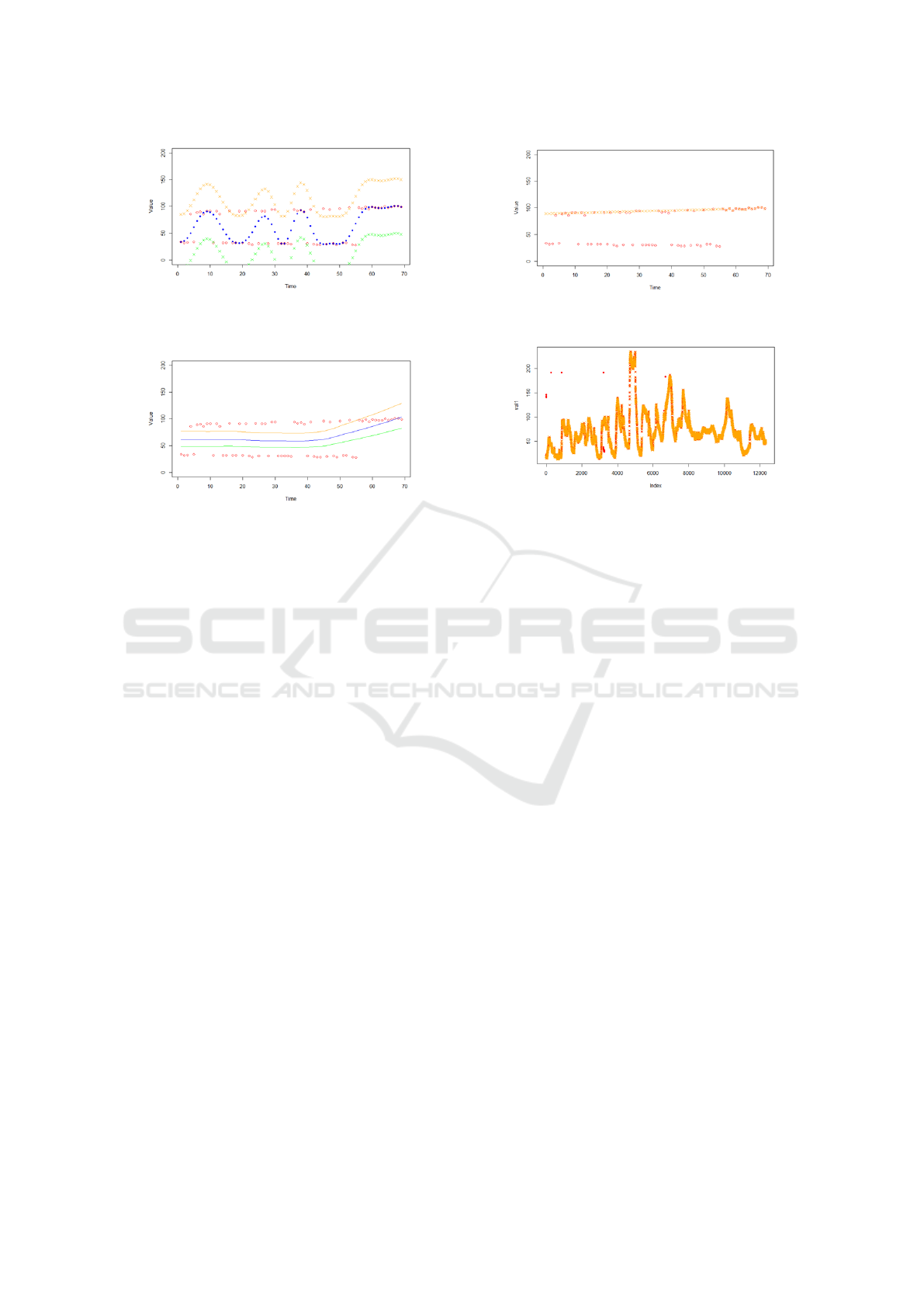
Figure 9: SVR for Phase-2: Outlier removal using SVR

after trend separation. Overﬁtting occurs, failing to remove

outliers.

Figure 10: Loess for Phase-2: Outlier removal using Loess

after trend separation. Loess prevents overﬁtting while suc-

cessfully removing most outliers.

median, may not be ideal as they do not always re-

ﬂect real values. A more suitable approach in this case

is mode replacement, where the most frequent value

is used for imputation, ensuring greater accuracy in

maintaining data integrity.

2.5 Step-5: Imputation of NULL Values

In previous phases, most outliers were replaced with

NULL values, which now need to be approximated

to make the dataset complete. Common imputation

techniques like Mean, Median, and Mode replace

NULLs with a single value, which may not sufﬁ-

ciently capture the underlying trends in non-linear

data.

While Median and Mode provide better estimates

than the Mean, they still fail to account for non-

linearity. Given the non-linear nature of the dataset, a

more suitable approach is required. Since SVR tends

to overﬁt but is effective for non-linear predictions,

we apply it to the subsets for imputation based on pre-

dicted results, as shown in Figure 11.

Figure 11 demonstrates that SVR closely matches

the imputed data with the actual data for one subset.

This technique is then applied across all subsets, en-

suring both outlier removal and accurate NULL value

imputation in a fully automated process.

As shown in Figure 12, the process successfully

removes global outliers, while remaining contextual

and collective outliers are identiﬁed. The ﬁnal dataset

provides an accurate representation with minimal out-

Figure 11: SVR for Data Imputation: Original data (red)

and cleaned data (orange).

Figure 12: Clean Data after IQR Phase-1: Original data

(red) and cleaned data (orange).

liers and properly imputed values.

3 EXPERIMENTS AND RESULTS

3.1 Test Setup

The algorithm was tested using data from an air qual-

ity monitoring system deployed in an ofﬁce environ-

ment. Sensors continuously collected data at a 120-

second sampling rate, which was stored on a local

gateway and transmitted to a cloud server for long-

term storage. The dataset comprised 12,312 real-time

air pollution data points. To efﬁciently manage this

high volume of data, we implemented a serverless

real-time data analytics platform for edge computing

(Nastic and Rausch, 2017).

Machine learning techniques, including Support

Vector Regression (SVR) and Loess, were applied to

detect and handle both contextual and collective out-

liers within the dataset (Mahdavinejad et al., 2018).

These techniques were crucial for ensuring data accu-

racy and addressing the challenges posed by outliers

in a real-time processing environment.

The experiments were conducted on a laptop with

a Core i7-4750 Mobile CPU (2.00 GHz) and 16 GB

of RAM, utilizing the R Programming Language for

the algorithm implementation and analysis.

L2C: Learn to Clean Time Series Data

365

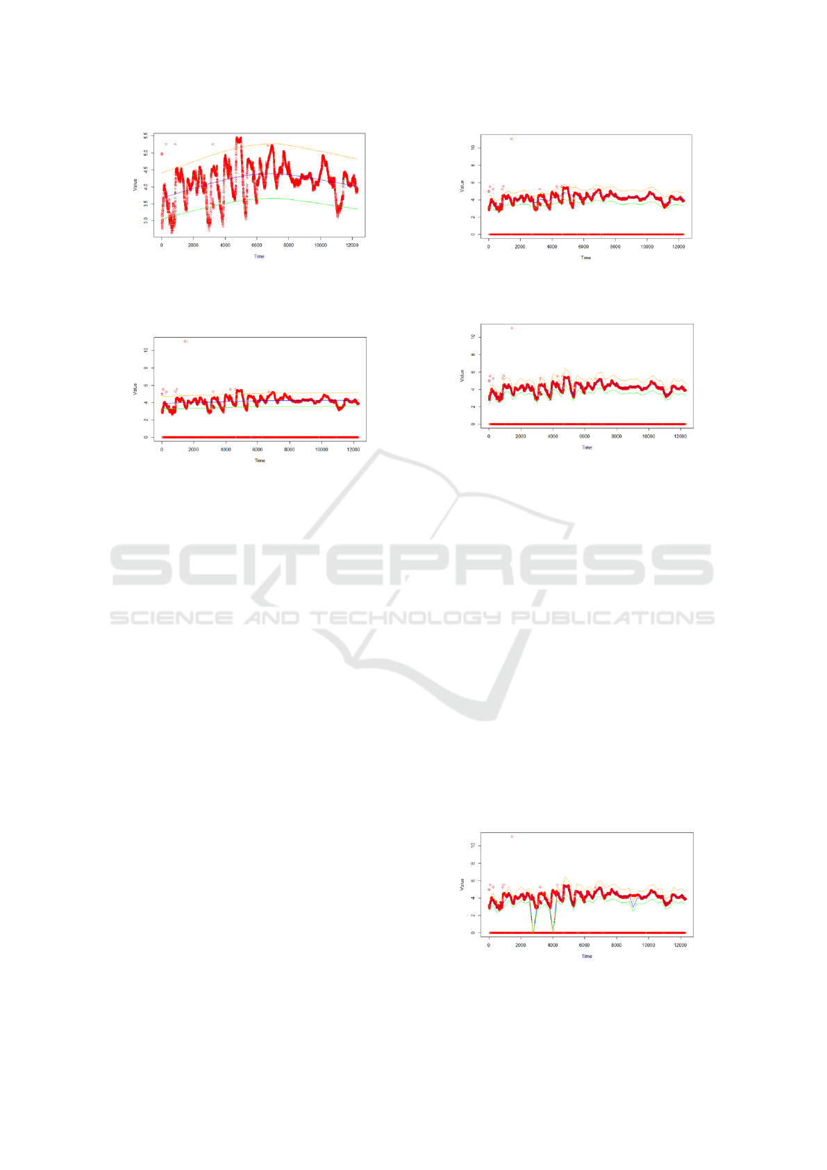
Figure 13: Data Cleaning Using Loess (span=0.75). Red

is original data, blue is predicted data, green represents the

lower limit, and orange the upper limit. Data beyond green

and orange is removed.

Figure 14: Data Cleaning Using Loess (span=2). Red is

original data, blue is predicted data, green represents the

lower limit, and orange the upper limit.

3.2 Standard Algorithm Results

We compared our multi-phase technique to standard

methods like Loess and ARIMA. ARIMA, a founda-

tional time series model (Box and Jenkins, 1976), per-

forms well with smaller, controlled datasets but strug-

gles with larger, more complex datasets due to its high

computational demands (Salman and Jain, 2019). In

contrast, SVR and Loess demonstrated better perfor-

mance in detecting outliers, especially in non-linear

data (Deng et al., 2005). By integrating these tech-

niques, L2C provides robust data cleaning for large-

scale IoT applications (Mahdavinejad et al., 2018).

Previous studies have also highlighted the efﬁcacy

of Support Vector Machines in time series prediction

(Muller et al., 1999).

In Figure 13, the standard Loess span of 0.75 re-

moves signiﬁcant portions of valid data while failing

to remove some outliers. This demonstrates inefﬁ-

ciency, as the model alters the dataset too drastically.

To improve accuracy, we experimented with different

span values.

As seen in Figure 14, increasing the span to 2

worsens the results, removing even more valid points.

Adjusting the span further was necessary to achieve a

balance between preserving the original data and re-

moving outliers.

The results improve signiﬁcantly when the span

is adjusted to 0.0075 (Figure 15). A span of 0.075

underﬁts, and lowering it further causes overﬁtting.

Figure 15: Data Cleaning Using Loess (span=0.075). Red

is original data, blue is predicted data, green is the lower

limit, and orange is the upper limit.

Figure 16: Data Cleaning Using Loess (span=0.0075). Red

is original data, blue is predicted data, green is the lower

limit, and orange is the upper limit.

Although 0.0075 does not remove as many outliers as

other spans, it preserves most of the valid data, mak-

ing it the best ﬁt. This conﬁguration minimizes outlier

presence while maintaining data integrity.

Compared to ARIMA, as shown in Figure 18, our

approach is more effective for large datasets. ARIMA

struggles to detect collective outliers and is inefﬁcient

due to its processing time and resource requirements

(Salman and Jain, 2019). To address this, we split the

dataset into 124 groups of 100 points each and per-

formed time series analysis on each subset. Although

this reduces processing time, the identiﬁed outliers

vary based on how the data is split, limiting full au-

tomation.

3.3 Test Results

We compared our multi-step technique with standard

methods for outlier detection and removal. Approx-

Figure 17: Data Cleaning Using Loess (span=0.00075).

Red is original data, blue is predicted data, green is the

lower limit, and orange is the upper limit.

IoTBDS 2025 - 10th International Conference on Internet of Things, Big Data and Security

366

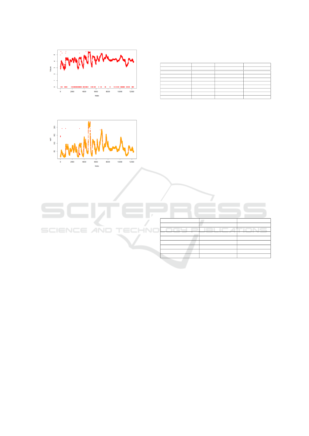
Figure 18: Data Cleaning Using ARIMA (Log Trans-

formed). Many outliers remain, including zero values, indi-

cating ARIMA’s limited cleaning performance.

Figure 19: Data Cleaning Using the two-phase s-SVR pro-

cess. The red is the original data, while orange represents

the cleaned data.

imately 8.78% of the dataset contained zero values,

making outlier detection essential. Initially, the In-

terquartile Range (IQR) rule was applied to eliminate

global outliers, but contextual and collective outliers

remained, as shown in Figure 8.

Next, we used Support Vector Regression (SVR)

to handle outliers more accurately, particularly for

non-linear data. Although SVR is computationally

intensive, it yielded better results. To optimize per-

formance, we applied split-SVR to reduce process-

ing time, which was effective for datasets with over

2.5% zero values, as demonstrated in Figure 10. Split-

ting the data into ﬁve sections with varying thresholds

helped in the removal of many contextual outliers.

We then applied trend analysis by calculating the

ﬁfth difference and merging subsets with fewer than

ﬁve points. This yielded 384 distinct trends. Loess

was applied to each trend, successfully removing col-

lective outliers, as shown in Figure 12.

Finally, SVR was used to overﬁt the sample and

impute values in place of outliers. Figure 13 shows

that the outliers were completely removed, and the

imputed data closely matched the actual values. This

process was repeated across all subsets to achieve

the most accurate data representation in an automated

manner.

Figure 14 illustrates the effectiveness of the multi-

phase process. The cleaned data ﬁts the original

dataset almost perfectly, with the data separated into

384 sets, each cleaned individually.

Table 1 summarizes the effectiveness of each tech-

Table 1: Proposed Technique vs Standard Technique for

Outlier Removal.

Method Global Outliers Contextual Outliers Collective Outliers

1082 14 34

Loess (Span=0.75) 100% 85.71% 14.71%

Loess (Span=0.075) 100% 78.57% 91.18%

Loess (Span=0.0075) 100% 85.71% 32.35%

Loess (Span=0.00075) 100% 7.14% 100%

Loess (Span=2) 100% 0% 97.06%

ARIMA 57.12% 14.29% 0%

IQR Multi-Phase 100% 85.71% 100%

Split-SVR Multi-Phase 100% 85.71% 100%

nique in removing different types of outliers. Loess

shows strong performance in removing global out-

liers, though it struggles with contextual and collec-

tive outliers. ARIMA performs poorly, especially

with collective outliers. Our multi-phase techniques,

IQR and split-SVR, successfully removed all types of

outliers.

For contextual outliers, reducing the Loess span

from 0.75 to 0.00075 improves removal, but overﬁt-

ting and underﬁtting issues arise. ARIMA also strug-

gles with contextual outliers, while our methods re-

move the majority of them effectively.

Our techniques also remove all collective outliers,

while Loess with spans 0.00075 and 2 achieves this

with some issues of overﬁtting and underﬁtting. Table

2 compares the methods’ impacts on actual data and

imputation.

Table 2: Effect on Actual Data and Imputation.

Method Actual Data Affected Data Replacement

Loess (Span=0.75) Yes No

Loess (Span=0.075) Yes No

Loess (Span=0.0075) Yes No

Loess (Span=0.00075) Yes No

Loess (Span=2) Yes No

ARIMA Yes No

IQR Multi-Phase No Yes

Split-SVR Multi-Phase No Yes

Table 2 illustrates that all methods affect actual

data, often removing valid points. Data imputation

can mitigate this, but only our techniques include im-

putation, which aims to replace removed points with

values close to the original.

Both of our techniques (IQR and split-SVR) per-

form equally well, suggesting that the second phase

(SVR) is more crucial than the ﬁrst. Given the time

required for the ﬁrst phase, we split the data into ﬁve

parts, which optimized performance. While s-SVR is

not fully automated, IQR is, so we prioritize using the

automated IQR technique for future applications.

4 SUMMARY AND CONCLUSION

This paper presented a multi-phase data cleaning ap-

proach that effectively addresses the challenges of

L2C: Learn to Clean Time Series Data

367

handling NULL values and outliers in univariate data.

Data quality is paramount in machine learning appli-

cations, as unreliable or unclean data can lead to poor

model performance. Our research aimed to overcome

these challenges by introducing a systematic method

that ensures cleaner, more reliable datasets, particu-

larly in applications like soil moisture sensors.

We classiﬁed outliers into three main types:

global, contextual, and collective. Each type re-

quires a different approach for detection and removal,

which is why traditional methods often fall short. Our

multi-phase approach integrates s-SVR (split-SVR)

and trend-based segmentation, followed by Loess and

regression analysis to remove outliers at each stage

of processing. By using s-SVR, we successfully re-

moved global and most contextual outliers while pre-

serving the integrity of the data. The segmentation

and regression steps handled the remaining outliers,

ensuring a comprehensive cleaning process.

The advantage of this approach is its ability to au-

tomate much of the data cleaning process, minimiz-

ing the need for manual intervention. Compared to

standard techniques like Loess or ARIMA, which ei-

ther underﬁt or overﬁt the data, our method provides

superior accuracy in removing anomalies without dis-

torting the original dataset. This makes it particularly

suitable for univariate time series data, where trends

and patterns must be preserved for reliable analysis.

4.1 Impact on Machine Learning

Models

The impact of this method on machine learning mod-

els is signiﬁcant. Clean, structured data ensures that

models perform better, with more accurate predic-

tions and fewer biases. In real-world applications,

such as soil moisture monitoring, having reliable data

leads to better decision-making and more efﬁcient re-

source management. Additionally, by removing out-

liers and imputing missing values, the model’s abil-

ity to generalize is improved, leading to better perfor-

mance in various predictive tasks.

4.2 Future Directions

While this research focuses on univariate data, there

is room to expand this technique to more com-

plex datasets. Future work could involve adapting

the multi-phase process for multivariate data, which

would open up new applications in ﬁelds such as

healthcare, telecommunications, and ﬁnance, where

data variability is high. Moreover, integrating this

approach into real-time systems and large-scale IoT

environments could prove invaluable for industries

requiring continuous monitoring and quick response

times.

Another promising area for future exploration is

the application of this method in deep learning and

large language models (LLMs). As these models

heavily depend on large, clean datasets, automating

data cleaning at this scale would greatly enhance

model performance, particularly in domains like natu-

ral language processing (NLP) and image recognition.

4.3 Conclusion

In conclusion, the multi-phase data cleaning method

we have proposed offers a comprehensive and auto-

mated solution to the critical challenge of handling

outliers and missing values in univariate datasets. By

removing global, contextual, and collective outliers

in successive stages, this approach signiﬁcantly en-

hances the quality of data used in machine learning

models. The method’s scalability and adaptability

make it applicable across various industries that rely

on univariate time series data.

Improving data quality is vital to ensuring the ac-

curacy and reliability of machine learning models, es-

pecially in ﬁelds where precision is critical. Investing

in data cleaning processes, as demonstrated in this re-

search, leads to better predictive models and more in-

formed decision-making, thus beneﬁting a wide range

of applications.

ACKNOWLEDGEMENTS

The authors would like to express their gratitude to

Dr. Rajan Nikam, whose expertise in mathematics

was invaluable in developing the mathematical frame-

work for this research. Their insights and guidance

signiﬁcantly contributed to the success of this work.

REFERENCES

Aggarwal, C. C. (2015). Outlier Analysis. Springer, Berlin,

1st edition.

Box, G. E. P. and Jenkins, G. M. (1976). Time Series Analy-

sis: Forecasting and Control. Holden-Day, San Fran-

cisco, 2nd edition.

Deng, Y.-F., Jin, X., and Zhong, Y.-X. (2005). Ensemble

svr for prediction of time series. In 2005 Interna-

tional Conference on Machine Learning and Cyber-

netics. IEEE.

Mahdavinejad, M. S., Rezvan, M., Barekatain, M., Adibi,

P., Barnaghi, P., and Sheth, A. P. (2018). Machine

learning for internet of things data analysis: A survey.

In Digital Communications and Networks. Elsevier.

IoTBDS 2025 - 10th International Conference on Internet of Things, Big Data and Security

368

Muller, K. R., Smola, J. A., Ratsch, G., Scholkopf, B., and

Kohlmorgen, J. (1999). Prediction time series with

support vector machines. In Scholkopf, B., Burges, C.

J. C., and Smola, A. J., editors, Advances in Kernel

Methods: Support Vector Learning, pages 243–254,

Cambridge, MA, USA. MIT Press.

Nastic, S. and Rausch, T. (2017). A serverless real-time

data analytics platform for edge computing. In IEEE

Internet Computing. IEEE.

Salman, T. and Jain, R. (2019). A survey of protocols

and standards for internet of things. In arXiv preprint

arXiv:1903.11549. arXiv.

L2C: Learn to Clean Time Series Data

369