Cost-Effective Strabismus Measurement with Deep Learning
Luis Felipe Araujo de Oliveira
a
, Jo
˜
ao Dallyson Sousa de Almeida
b
,
Thales Levi Azevedo Valente
c
, Jorge Antonio Meireles Teixeira
d
and Geraldo Braz Junior
e
N
´
ucleo de Computac
˜
ao Aplicada, Universidade Federal do Maranh
˜
ao (UFMA), S
˜
ao Lu
´
ıs, MA, Brazil
Keywords:
Strabismus, Convolutional Neural Network, Deep Learning, YOLO.
Abstract:
This article presents a new methodology for detecting and measuring strabismus. Traditional diagnostic meth-
ods in the medical field often require patients to visit a specialist, which can present challenges in regions
with limited access to strabismus experts. An accessible and automated approach can, therefore, support
ophthalmologists in making diagnoses. The proposed methods use images from the Hirschberg Test exams
and employ techniques based on Convolutional Neural Networks (CNNs) and image processing to detect the
limbus region and measure the brightness reflected in patients’ eyes from the camera’s flash. The method cal-
culates the distance between the limbus’s center and the reflected brightness’s center, converting this distance
from pixels to diopters. The results show the potential of these approaches, achieving significant effectiveness.
1 INTRODUCTION
Strabismus is an eye condition in which the eyes
are not correctly aligned and point in different di-
rections. This condition affects about 2% to 4% of
the global population (Hashemi et al., 2019) and is
often caused by abnormalities in binocular vision or
issues with the neuromuscular control of eye move-
ments. Strabismus can result in various complica-
tions, including permanent vision loss, visual field
defects, and impaired binocular vision, among other
problems(Buffenn, 2021).
The current diagnosis of strabismus primarily re-
lies on two tests: the Prismatic Cover Test (PCT),
also known as the Cover Test, and the Hirschberg
Test. During the PCT, the examiner alternately cov-
ers one eye while observing the other. They measure
the deviation in prismatic diopters (PD) by adjusting
the strength of the prism to restrict eye movement. In
the Hirschberg Test, the examiner shines a small light
into the patient’s eyes. They determine the angle of
the strabismus by measuring the distance between the
corneal reflection light reflection (CR) and the center
a
https://orcid.org/0009-0008-8717-4420
b
https://orcid.org/0000-0001-7013-9700
c
https://orcid.org/0000-0002-5429-4986
d
https://orcid.org/0000-0002-1842-486X
e
https://orcid.org/0000-0003-3731-6431
of the pupil. Both tests rely on the examiner’s exper-
tise and can introduce subjectivity.
There have been efforts to enhance the accuracy
of strabismus measurement and detection, as seen
in studies (Miao et al., 2020) and (Durajczyk et al.,
2023). However, these methods often require costly
virtual reality or specialized equipment, which can be
impractical for small clinics in rural areas.
In recent years, researchers have widely used con-
volutional neural networks (CNN) for various classifi-
cation and detection tasks (Li et al., 2022) due to their
strong ability to generalize across different data types.
This capability enables them to handle complex ob-
ject detection scenarios, such as identifying cars or
human faces. Additionally, studies demonstrate that
CNNs outperform traditional computer vision meth-
ods in classification and detection tasks (O’Mahony
et al., 2020).
Therefore, the present work aims to address the
challenges of strabismus diagnosis by proposing a
methodology for detecting this condition. Building
upon the Hirschberg Test, it leverages advancements
in Convolutional Neural Networks (CNNs) and im-
age processing techniques to improve accuracy, ac-
cessibility, and cost-effectiveness. By integrating au-
tomated detection capabilities, these proposed ap-
proaches reduce the reliance on specialized equip-
ment and the need for expert examiners, making
them particularly suitable for areas with limited ac-
Araujo de Oliveira, L. F., Sousa de Almeida, J. D., Valente, T. L. A., Teixeira, J. A. M. and Braz Junior, G.
Cost-Effective Strabismus Measurement with Deep Learning.
DOI: 10.5220/0013438200003929
Paper published under CC license (CC BY-NC-ND 4.0)
In Proceedings of the 27th International Conference on Enterprise Information Systems (ICEIS 2025) - Volume 1, pages 593-604
ISBN: 978-989-758-749-8; ISSN: 2184-4992
Proceedings Copyright © 2025 by SCITEPRESS – Science and Technology Publications, Lda.
593

cess to ophthalmological resources, with the hopes
of making strabismus diagnosis widely available and
cheaper.
This study utilizes a comprehensive dataset of
Hirschberg Test images collected under controlled
and real-world conditions to evaluate the proposed
methodologies effectively. The evaluation metrics in-
clude precision, recall, and computational efficiency,
providing a thorough assessment of the performance
of the proposed methods. This work aims to con-
tribute to the field of ophthalmology by offering scal-
able and practical solutions for strabismus detection.
These advancements can potentially improve early di-
agnosis and treatment outcomes, especially in under-
served regions, thus addressing a critical gap in global
eye care.
2 RELATED WORK
In recent years, there has been a growing effort to
automate strabismus measurement, given the serious-
ness of the problem and the negative consequences of
untreated strabismus.
In (Almeida, 2015), researchers propose a pio-
neering method for preliminary screening and assist-
ing in diagnosing strabismus in digital images, uti-
lizing a dataset of 40 strabismic patients and 5 non-
strabismic individuals. They first segment the fa-
cial region based on the color range of human skin.
Within the area defined by the filter, they employ Sup-
port Vector Machine (SVM) algorithms, geostatisti-
cal functions, histogram equalization, and the circular
Hough Transform to locate both eyes accurately. Us-
ing an additional Hough Transform, they identify the
limbus and the CR within the eye region. The detec-
tion types of strabismus were (ET), exotropias (XT),
hypertropias (HT), and hypotropias (HoT), with the
method achieving an accuracy of 88% and 100% for
ET and XT (horizontal deviations), respectively, and
80.33% and 83.33% for HT and HoT (vertical devia-
tions), respectively. The total mean error in diopters
was 5.6∆ and 3.83∆ for horizontal and vertical devia-
tions, respectively.
In (Cheng et al., 2021), a school nurse conducted
vision screening in an elementary school using spe-
cialized equipment and the EyeTurn app, referenced
in (Pundlik et al., 2019), which outputs information
about eye location and strabismus measurement (in
diopters). Following a predefined protocol, an ex-
pert evaluated whether the software correctly identi-
fied image features such as the iris and corneal re-
flection. In the first moment, the researchers used a
threshold of 2.4 ∆ (strabismus detected by the app) to
decide which patients required in-person cover testing
with a specialized eye doctor. They successfully ob-
tained at least one measurement from the app for 93%
of the children. Of these, 40 children were flagged
for a prism alternate cover test, and 6 were confirmed
to have strabismus. The study established the app’s
optimum threshold for detecting strabismus to be 3.0
∆, achieving a sensitivity of 83% and a specificity of
76.5%.
In (S¸
¨
ukr
¨
u Karaaslan et al., 2023), a pre-trained
Key-Point detection model, Mediapipe, a frame-
work implementation of the model developed in
(Bazarevsky et al., 2019), determines the eye iris re-
gion. Next, the CR is segmented using a binary seg-
mentation along Otsu’s algorithm for determining the
threshold; for the pupil, the image is converted from
grayscale to HSV, zooming in the iris for better detec-
tion of the pupil, which is segmented using an arbi-
trary threshold determined by the authors and by se-
lecting the minimum enclosing circle of the region.
Strabismus is measured based on the distance be-
tween the pupil and CR centers. The method consid-
ers that the correct detection of the CR and the cornea
is a successful measurement, given that hypothesis the
authors achieved 90% accuracy for right and 91% ac-
curacy for left iris detection, 98% accuracy for CR
detection and a maximum error of ± 2° in measure-
ments. Average measurement error or standard devi-
ation were not specified.
(Dericio
˘
glu and C¸ erman, 2019) analyzed 1,022
photographs with a resolution of 3264x2448 from
15 orthophoric subjects with known gaze angle and
imaging distance. They developed a smartphone ap-
plication allowing users to mark the limbus and the
corneal light reflex manually. The application then
calculated the distance from the geometric center of
the cornea to the light reflex (RD), the corneal diam-
eter (CD), and the interpupillary distance (IPD). The
study presented two parts. In the first part, the re-
searchers measured each patient’s RD/CD ratio and
used it in a regression model to develop a non-linear
equation for estimating gaze angles. They incorpo-
rated the IPD to calculate a trigonometric function
suitable for converting pixels to millimeters based on
imaging distance. In the second part, they applied
these equations to 572 photographs of strabismus pa-
tients to calculate deviations based on their RD/CD
ratio and IPD. They then compared these results with
measurements taken by a double-masked strabismus
specialist using the Krimsky or Prism Cover Test. The
paper achieved high correlation between estimated
measurements and the specialist, with r = 0.966 and
P < 0.001, mean error of the estimated gaze angle
0.03∆ ± 4.60∆ and average error −0.68∆ ± 6.1∆; the
ICEIS 2025 - 27th International Conference on Enterprise Information Systems
594

reliability of the method was high, given Cronbach’s
α = 0.983.
Given an extensive search of the literature, it is
clear that precise object detection is one of the main
bottlenecks for automatic methods of strabismus mea-
surement and can be a decisive factor for the correct
calculation. In (Almeida, 2015), feature-based im-
age processing algorithms are used to detect the lim-
bus and the CR for measurement; the method does
achieve reliable results but is inviable for resource-
restricted situations due to the cost of all of the image
processing required to detect the limbus and the CR.
In (S¸
¨
ukr
¨
u Karaaslan et al., 2023) after the initial iris
detection using a Deep Learning model, the rest of
the method also relies on image processing to detect
the pupil and the CR; the pupil is much more difficult
to detect than the limbus due to its variable but much
smaller size compared to limbus, a fact that can in-
crease the error rate of such method extensively when
the patient wears corrective lenses(the lenses would
generally distort the color of or partially occlude the
pupil).
Alternative methods for automatic detection of
strabismus involve using smartphone apps, due to the
great availability of smartphones and ease of use of
such apps, as in (Cheng et al., 2021), where a nurse
was only required to align the patient’s eyes with rect-
angles displayed in the app’s interface. In (Dericio
˘
glu
and C¸ erman, 2019) the app was used to obtain the RD,
CD and IPD whilst the strabismus calculation was in-
ferred from this data. Both methods required human
input, even if not requiring knowledge of strabismus
measurements, but achieved significant practical re-
sults, either with high correlation with specialist mea-
surements or high specificity and sensitivity.
Even though (Almeida, 2015) evaluates five dis-
tinct gaze positions, it employs an extensive image-
processing pipeline and parameterized feature extrac-
tion, increasing both parametrization and computa-
tional costs. In contrast, our proposed solution har-
nesses convolutional neural networks (CNNs) to au-
tomatically detect the corneal reflex and the limbus,
eliminating the need for additional human input or
specialized knowledge of strabismus measurement.
Moreover, our approach also evaluates five gaze posi-
tions yet does so with greater efficiency and scalabil-
ity, making it more suitable for real-world screening
scenarios where time and resources are limited.
However, this work aims to create a scalable
and practical solution for strabismus measurement,
one that does not require human-input, any knowl-
edge of strabismus measurement, together with cost-
effectiveness related both to speed and precision of
measurements.
3 MATERIALS AND METHODS
In this section, we will discuss the dataset, used net-
work and details of this work’s method, along with
the specifics of strabismus calculation.
3.1 Dataset
The dataset is the same as used in (Almeida, 2015),
and comprises of 277 images with a resolution of
1536x2048 from 45 patients of various sexes and
ages. These images capture five distinct gaze posi-
tions: PP (Primary Position of Gaze), LEVO (eyes
looking to the left), DEXTRO (eyes looking to the
right), SUPRA (eyes looking upward), and INFRA
(eyes looking downward). Figure 1 illustrates these
gaze positions. For testing purposes, only the images
in these 5 standard gaze positions were used for test-
ing as noted in Section 4, despite some patients having
images in variations of the 5 standard positions (e.g:
patients looking both upward and to the left).
(a) .
(b) . (c) . (d) .
(e) .
Figure 1: a) SUPRA, b) LEVO, c) PP, d) DEXTRO, e) IN-
FRA.
Researchers manually annotated all images and
used them for training the network. For the testing
phase, we excluded four patients who lacked com-
plete annotations from the physician.
3.2 YOLO (You Only Look once)
YOLO, which stands for “You Only Look Once,” is
a convolutional neural network designed for real-time
object detection. It introduces a novel approach to de-
tection initially proposed by (Redmon et al., 2015).
Unlike traditional methods that treat object detection
as a classification problem, YOLO treats it as a re-
gression problem.
YOLO consists of a unified model in which a sin-
gle network predicts the location of objects and their
corresponding classes. This design allows YOLO to
operate at remarkable speeds; for instance, YOLOv8
can process images at 150 frames per second (FPS)
Cost-Effective Strabismus Measurement with Deep Learning
595

with an Average Precision Across Scales (APAS) of
52.7. These results were achieved using the COCO
(Common Objects in Context) challenge dataset (Lin
et al., 2014) and executed on NVIDIA RTX 3090
GPU.
Although researchers initially designed YOLO for
real-time detection in videos, they have demonstrated
its effectiveness for object detection in images as well
(Varghese and M., 2024). In its eighth version, the
network produces three outputs: the first includes the
coordinates of the detected bounding box (bbox), its
confidence score, and the class of the detected object
within that region. The model calculates the confi-
dence score of the bbox based on the estimated prob-
ability that the region belongs to the specified class.
This work employs YOLOv8, as outlined in (Vargh-
ese and M., 2024).
The YOLOv8 network has two main components:
the backbone and the head. The backbone, a con-
volutional neural network (CNN), extracts a feature
map from the input and provides context at multi-
ple levels of representation for the rest of the net-
work. In YOLOv8, engineers base the backbone on
the EfficientNet-B4 architecture (Tan and Le, 2019).
Meanwhile, the head utilizes the feature map pro-
duced by the backbone as input for additional convo-
lutions and upsampling layers. Ultimately, it culmi-
nates in final convolutions that perform object classi-
fication and localization.
3.3 Method
This work employs the YOLO model for detecting
both corneal reflection and limbus due to its robust-
ness and effectiveness in object detection, as outlined
in Section 4.1. We train the YOLOv8 network on the
dataset described in 3.1 to accurately identify the lim-
bus and the corneal reflection point in the patient’s im-
age. This identification enables us to calculate strabis-
mus using the coordinates obtained from the bound-
ing boxes. Figure 2 illustrates our method.
Initially, we divided the patient’s image into two
halves along the vertical axis (we blurred the image in
the figure to anonymize the patient). We then perform
inference on both halves of the image. If the network
detects at least two bounding boxes for the limbus and
two for the corneal reflection, we proceed with the
method; otherwise, we consider it an error. Typically,
the number of bounding boxes exceeds the minimum
required, so we must filter which ones to use. We
check for all limbus bounding boxes if there are any
CR bounding boxes, if there are not any, the bounding
box is excluded, with the same logic being applied to
CR bounding boxes. In most cases (except for specific
exceptions), the corneal reflection is contained within
the limbus.
Finally, the corneal reflection bounding boxes are
sorted based on their distance to the limbus. This
is because erroneously detected corneal reflection
bounding boxes are very likely to be farther from any
limbus bounding box. The two pairs of bounding
boxes (corneal reflection and limbus) with the small-
est distances with respect to each other are selected,
following the hypothesis that if low-quality bound-
ing boxes still remain after the exclusion process, the
model will likely still detect the correct limbus bound-
ing boxes close to the corneal reflection bounding
boxes.
3.3.1 Strabismus Calculation
After identifying the bounding boxes for both eyes
and corneal reflection using the procedure above, we
compute the strabismus angles through the following
steps:
1. Identify the Fixating Eye: calculate the Eu-
clidean distance between the center of the limbus
and the corneal reflection for each eye. The eye
with the smaller distance is considered the fixat-
ing eye.
2. Compute the Deviated Eye Displacement: for
the other (deviated) eye, compute the horizontal
(HD
pixel
) and vertical (V D
pixel
) components of
the distance between the center of the limbus and
the corneal reflection.
3. Convert Pixels to Millimeters: use the following
equation to convert pixel distances to millimeters:
pixel
MM
= Limb
adult
/Diam
f ix
where Diam
f ix
is
the diameter of the fixating eye in pixels (the
bounding box’s width for horizontal calculations
and height for vertical calculations). Limb
adult
represents the average adult limbus size (Khng
and Osher, 2008). Consequently:
HD
mm
= HD
pixel
∗ pixel
MM
V D
mm
= V D
pixel
∗ pixel
MM
4. Convert Millimeters to Diopters: finally, con-
vert the distances in millimeters to diopters using
the conversion constant delta = 15, as established
in (Schwartz, 2006) and (Almeida, 2015):
HD
diop
= HD
mm
∗ delta
V D
diop
= V D
mm
∗ delta
By integrating the CNN-based detection (Sec-
tion 3.3) with the strabismus calculation steps out-
lined here, our approach delivers an automated and
efficient framework for reliably measuring strabismus
in clinical or field settings.
ICEIS 2025 - 27th International Conference on Enterprise Information Systems
596

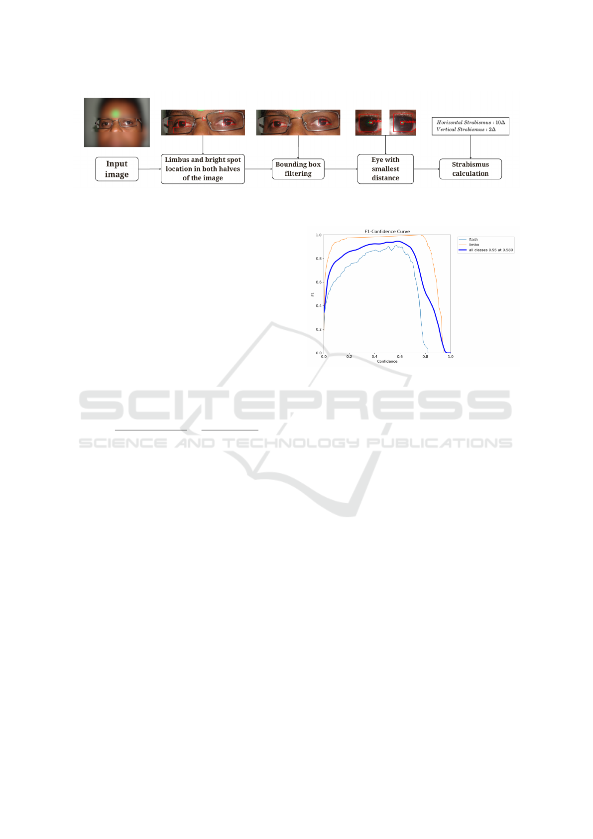
Figure 2: CNN-based strabismus calculation.
4 RESULTS AND DISCUSSION
We divided the experimental outcomes into training
and testing to provide a comprehensive analysis of
both phases.
4.1 Training
We evaluated the training performance of the model
using Precision, Recall, and the F1-Score metrics.
The F1-Score represents the harmonic mean of Pre-
cision (the ratio of true positives to all predicted pos-
itives) and Recall (the ratio of true positives to all ac-
tual positives). Mathematically, the F1-Score is de-
fined as:
F
1
= 2
precision ∗ recall
precision + recall
=
2t p
2t p + f p + f n
(1)
where t p denotes true positives (bounding boxes
with an Intersection over Union (IoU ≥ 0.5); f p de-
notes false positives (IoU < 0.5), and f n indicates
false negatives (the background being mislabeled as
a valid bounding box). The F1-Score ranges from 0
to 1, with higher values indicating better model per-
formance.
We conducted training on Google Colab (Google,
2023) (version 2024-11-11), a cloud-computing plat-
form for Machine Learning and Data Analysis, using
an Ubuntu 22.04 LTS virtual machine equipped with
an Nvidia T4 15 GB GPU. The model ran under the
Ultralytics (Jocher et al., 2023) framework (version
8.1.17) and used 2 training classes, limbo and flash
for the limbus and CR, respectively.
In the first training stage, we split the dataset (Sec-
tion 3.1) into 70% for training, 10% for validation,
and 20% for testing. We froze 15 out of 21 network
layers and trained for 39 of the planned 50 epochs, im-
plementing early stopping after 10 epochs. We used
a batch size of 3, an image resolution of 1600x1600 ,
optimizer with an initial learning rate of lr
0
= 0.01.
The final learning rate was set to lr
f
= 0.01 ∗ lr
0
,
following the Ultralytics scheduling strategy, which
Figure 3: F1-Score training curve.
starts with a higher learning rate and progressively
decreases it after each epoch. We applied data aug-
mentation online, employing transformations such as
saturation and hue adjustments, translation, scaling,
horizontal flipping, and partial image erasure through
the Ultralytics Python framework.
On the validation set, this training process
achieved a Precision of 0.972, a Recall of 0.474 and
a F1-Score of 0.637 on validation. Figure 3 exem-
plifies the performance differences between flash and
limbus detection, due to the higher amplitude of the
limbus class curve in the graph; the flash class had
worse performance, as denoted by the lower ampli-
tude in the plot, possibly due to other bright spots
present in some images, as discussed in Section 4.3.
Figure 4 shows precision and recall at varying thresh-
olds of IoU, with a satisfying performance for limbus
and a lower performance for the flash class. These re-
sults prompted the authors to further train the model
with 5-fold cross-validation to enhance the model’s
detection capabilities, as will be discussed.
In the second stage of training, we employed 5-
fold cross-validation (Refaeilzadeh et al., 2009), with
a 70%–30% split for training and testing, respectively.
We applied transfer learning at each training session,
using the weights from the previous session (Zhuang
et al., 2019). The first session in this stage initialized
its weights from the first training stage. Each session
was trained for 20 epochs, with early-stopping of 5
Cost-Effective Strabismus Measurement with Deep Learning
597

Figure 4: Precision-recall training curve.
epochs, retaining other hyperparameters from the ini-
tial training. Table 1 presents the results for each test
fold.
Table 1: Table with results respective to each fold and aver-
age metrics.
Test Fold Precision Recall F1-Score
FOLD 1 0.954 0.983 0.968
FOLD 2 0.949 0.980 0.964
FOLD 3 0,948 0.956 0.952
FOLD 4 0.963 0.965 0.964
FOLD 5 0,944 0.967 0.955
AVERAGE 0.952 0.970 0.961
Results were satisfactory both for classification
and bounding box localization, given high average
Precision, Recall and F1-Score. The last training re-
sults showed a good promise for precise CR and lim-
bus detection.
4.2 Test Results
We evaluated the model using the respective test fold
from each 5-fold cross-validation session, thereby
minimizing potential training bias. We also excluded
patient images that lacked strabismus annotations,
since these images could not be evaluated for mea-
surement error and patient images in non-standard
gaze positions, as the specialist had to ask some pa-
tients to look to the right and to the left when in the
INFRA and SUPRA positions. To make the quantity
of images in each position more balanced, such im-
ages were excluded. Results are evaluated with the
following metrics: Mean Absolute Error (MAE) in
prismatic diopters, Pearson’s correlation coefficient
(CORR) and amount of images that passed to the
measurement stage (QUANT).
Results relative to 213 valid images (i.e., images
with specialist annotations in all five standard gaze
positions), yielded 213 valid detections, correspond-
ing to an 100% detection rate. Test results took
around 100ms to 500ms. Table 2 shows the method
results for all positions.
Table 2: Average results per position.
METRICS
Position MAE TOTAL MAE H MAE V CORR H CORR V QUANT
PP 9.18 ± 8.09 12.81 ± 8.99 5.55 ± 3.65 0.65 0.2 42
DEXTRO 17.14 ± 29.19 27.32 ± 37.2 6.96 ± 6.94 0.25 0.47 43
LEVO 11.1 ± 15.41 16.29 ± 19.64 5.91 ± 4.26 0.57 0.35 43
SUPRA 14.76 ± 18.27 19.38 ± 22.33 10.13 ± 9.32 0.46 0.33 43
INFRA 32.91 ± 69.78 28.91 ± 44.53 36.92 ± 80.35 0.5 0.34 42
AVERAGE 17.02 ± 28.15 20.94 ± 26.54 13.09 ± 20.9 0.48 0.34 213
Given the high standard deviation in the overall
results from Table 2, also evidenced in the Bland-
Altman plot in Figure 5, we filtered out selected pa-
tients to achieve a more accurate analysis. Specifi-
cally, we removed cases where errors exceeded 2 stan-
dard deviations from the mean, because such high er-
rors usually denoted cases where the CNN detected
the CR very far in the image or the limbus was lat-
erally or vertically occluded, as will be discussed in
Section 4.3
Figure 5: Bland-Altman plot for the whole test set and all
positions, with horizontal and vertical strabismus. Mean
denote by red line, 95% Confidence Interval denoted by
dashed lines.
It can be observed from the results in Table 3 that
the LEVO position had the best result, with an aver-
age MAE of 7.18 ± 6.09 prismatic diopters. A reason
for such result is that most patients in the dataset have
some form of horizontal strabismus and when asked
to look to the right or to the left, the deviated eye be-
comes more visually perceptible to the CNN, also the
CR in the deviated eye becomes more dislocated in
some patients. Figure 6 illustrates a good measure-
ment in the LEVO position, with 3∆ and 3∆ of error
in horizontal and vertical measurements, respectively.
Table 3: Filtered results per position.
METRICS
Position MAE TOTAL MAE H MAE V CORR H CORR V QUANT
PP 7.48 ± 5.45 10.13 ± 5.15 4.84 ± 3.14 0.76 0.42 33
DEXTRO 9.76 ± 9.97 14.84 ± 11.14 4.68 ± 3.3 0.46 0.53 35
LEVO 7.18 ± 6.09 9.92 ± 6.8 4.43 ± 2.61 0.79 0.36 35
SUPRA 9.75 ± 7.67 12.16 ± 8.06 7.35 ± 4.54 0.8 0.63 34
INFRA 8.22 ± 6.95 11.46 ± 7.52 4.98 ± 3.34 0.58 0.47 35
AVERAGE 8.48 ± 7.23 11.7 ± 7.73 5.26 ± 3.39 0.68 0.48 172
The PP position had the second best result on av-
erage, losing to the LEVO position in the total aver-
age by less than 1∆. The PP position is often con-
sidered the easiest for measurement, since the eye-
ICEIS 2025 - 27th International Conference on Enterprise Information Systems
598

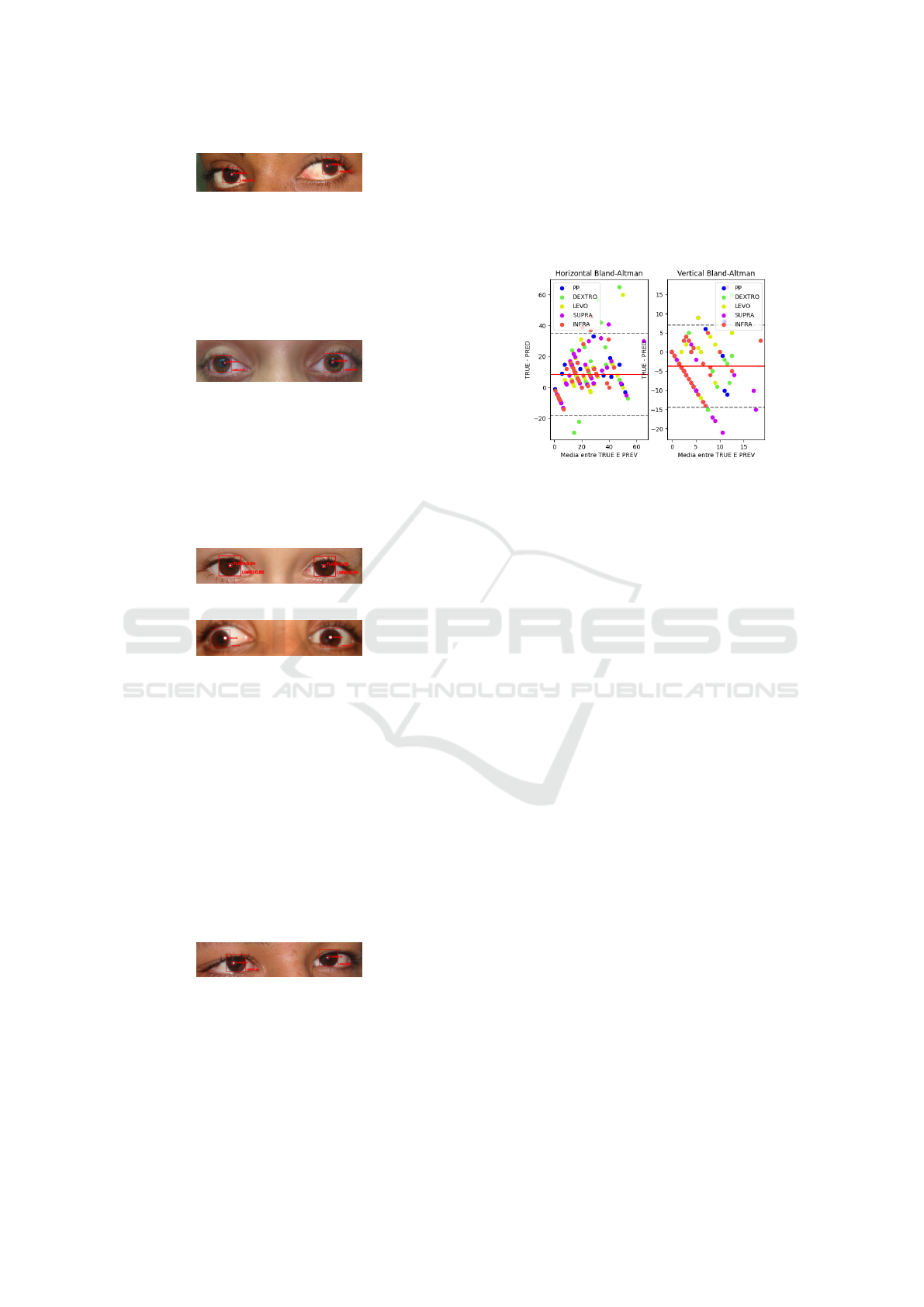
Figure 6: Patient 016 with a good measurement in the
LEVO position.
lids are more open and the patient is attempting to fix
the gaze directly into an object in front of them. Fig-
ure 7 illustrates a good measurement in the PP posi-
tion, with 3∆ and 5∆ of error in horizontal and vertical
measurements, respectively.
Figure 7: Patient 014 with a good measurement in the PP
position.
The SUPRA and INFRA positions had results
with an average error of 9.75 ± 7.67∆ and 8.22 ±
6.95∆, respectively. These positions can have worse
results since the limbus might be less visible in certain
patients, as discussed in Section 4.3. Figures 8 and 9
illustrate measurements in these positions.
Figure 8: Patient 001 in the SUPRA position.
Figure 9: Patient 006 in the INFRA position, error of 0∆ in
horizontal and error of 3∆ in vertical measurements.
The DEXTRO position had the worst results out
of all positions, with an average error 2.58∆ higher
than the LEVO position, a discrepancy similar to the
one between the INFRA and SUPRA position (The
SUPRA position being 1.53 ∆ worse worse on aver-
age than the INFRA position). Such differences can
be explained due to the acquisition of images not fol-
lowing a specific protocol, in order to simulate real-
world acquisitions, leading to differences between op-
posite positions that can diminish or increase mea-
surement error. Figure 10 illustrates patient 033 with
an error of 4∆in horizontal and error of 4∆ in vertical
measurements.
Figure 10: Patient 033 in the DEXTRO position.
As shown in Table 3 and in Figure 11, filtering
out these problematic cases significantly reduced the
standard deviation and improved overall results. The
vertical and horizontal MAE for most positions de-
creased below 10 ∆, aligning with the maximum er-
ror tolerance for specialist measurements reported in
(Choi and Kushner, 1998). The number of detected
images dropped from 213 to 172 after filtering, cor-
responding to 62.1% of the total dataset or 80.1% of
valid images. Despite this reduction, the lower vari-
ance in the metrics underscores the enhanced reliabil-
ity of the final analysis.
Figure 11: Bland-Altman plot with filtered results. Mean
denoted by red line, 95% Confidence Interval denoted by
dashed lines.
To assess the main method’s measurement perfor-
mance, the authors implemented two other strabismus
measurement methods. Both methods use the detec-
tions by the YOLO model as basis.
The first method comprises of several image pro-
cessing algorithms applied in sequence to try to es-
timate a circle that would be that would be consid-
ered the limbus. For this method the limbus bounding
boxes obtained by YOLO were used as input, extend-
ing the bounding boxes dimensions by 10%, then con-
verting the image to grayscale according to the equa-
tion:
Y = 0.299 · R + 0.587 · G + 0.114 · B
Where Y is the final pixel value in grayscale,
and R, G, and B are the red, green, and blue values
in the RGB scale, respectively. After converting to
grayscale, some image processing techniques are ap-
plied sequentially. A Difference of Gaussian (DoG)
is applied to emphasize the contours of the limbus.
Next, the unsharp masking algorithm, as described in
(Petrou and Bosdogianni, 1999), is used to enhance
the sharpness of the image. The Canny edge detec-
tion algorithm ((Canny, 1986)) is then executed, with
contours smaller than 20 px in perimeter being ex-
cluded. A custom mask is applied to the result of the
edge detection, the mask consisting of applying two
circular binary masks (matrices) to the image and re-
taining only the pixels located between the two circu-
lar masks, thereby excluding unwanted artifacts and
preserving the approximate region where the limbus
is located. The mask follows the formula below:
Cost-Effective Strabismus Measurement with Deep Learning
599

Mask(x,y) = E(x,y) & notI(x, y)
Result = Image & Mask(x, y)
Where E(x,y) is the larger-radius circular mask
(outer), I(x, y) is the smaller-radius circular mask (in-
ner), and Mask(x, y) is the mask to be applied to the
image, leading to only the contours between the two
masks remaining. After this step, the Hough Trans-
form is applied for detecting the limbus, as imple-
mented in (Valente et al., 2017), limiting angles to
between 60° and 120° for the top part of the circle and
240° to 300° for the bottom. This restriction accounts
for cases where the patient’s eyelid or glasses obscure
these regions of the limbus, potentially causing incor-
rect detections. The algorithm returns the most voted
circle in the image, which is then converted into a
square bounding box (height and width equal to the
circle’s radius), with the center corresponding to the
detected circle’s center. Strabismus is then calculated
based on this bounding box, as noted in Section 3.3.1.
It is worth noting that the parameters for the perimeter
filter, unsharp masking algorithm, and Hough algo-
rithm were chosen using a genetic algorithm (SHADE
algorithm) implemented in the Python optimization
library Mealpy 3.0.1 (Van Thieu and Mirjalili, 2023),
with a objective function of F = 0.5∗MAE +0.5∗SD,
where MAE is the Mean Absolute Error and SD is the
standard deviation, optimized for a subset of 10 pa-
tients taken from the training folder of the first train-
ing phase of the YOLO model. The optimization al-
gorithm is based on the article by (Tanabe and Fuku-
naga, 2014). Table 4 shows the results obtained by
this method and Figure 12 shows the main steps of
the method.
Figure 12: Hough Transform-based method for strabismus
calculation.
Table 4: Metrics table for the Hough Method.
METRICS
Position MAE TOTAL MAE H MAE V CORR H CORR V QUANT
PP 11.91 ± 6.77 12.69 ± 7.33 11.14 ± 5.27 0,514 0,216 33
DEXTRO 12.49 ± 9.86 13.58 ± 10.74 11.41 ± 7.45 0,626 0,286 36
LEVO 10.34 ± 7.25 12.23 ± 8.31 8.44 ± 4.76 0,502 0,356 33
SUPRA 12.15 ± 6.87 10.94 ± 6.6 13.37 ± 6.19 0,732 0,512 34
INFRA 13.96 ± 10.13 14.2 ± 9.66 13.71 ± 8.42 0,416 0,462 34
AVERAGE 12.17 ± 8.18 12.73 ± 8.53 11.62 ± 6.42 0,558 0,3664 170
Another method created for comparison consists
of using the bounding boxes provided by YOLO as in-
put and passing them to the Segment Anything Model
(SAM), as described in (Kirillov et al., 2023). In the
referenced article, the model is trained on a variety
of segmentation masks obtained and validated by the
authors, creating the SA-1B dataset with 1 billion seg-
mentation masks across various semantic levels. The
large volume of data improves the network’s gener-
alization, making it applicable to real-world contexts
rather than just benchmarks. In this method, SAM
was used to predict segmentation masks for each lim-
bus Region of Interest (ROI). The method starts with
the ROI detected by YOLO, performing detection
within it. After the SAM model completes its predic-
tion, the bounding box of the largest detected area is
considered to represent the limbus. The calculation of
strabismus then continues using the limbus detected
by SAM. Table 5shows the SAM method’s results.
Table 5: Metrics table for the SAM Method.
METRICS
Position MAE TOTAL MAE H MAE V CORR H CORR V QUANT
PP 88.84 ± 54.99 73.34 ± 18.03 104.34 ± 71.29 0,356 0,228 33
DEXTRO 107.13 ± 83.25 69.71 ± 25.54 144.55 ± 96.33 0,206 0,44 35
LEVO 87.57 ± 35.59 85.37 ± 38.77 89.77 ± 27.29 0,474 0,392 35
SUPRA 74.01 ± 22.43 64.85 ± 18.45 83.16 ± 19.7 0,372 0,49 35
INFRA 73.74 ± 23.64 65.34 ± 15.67 82.15 ± 24.06 0,262 0,51 33
AVERAGE 86.26 ± 43.98 71.72 ± 23.29 100.79 ± 47.74 0,334 0,412 171
It can be observed from the results that the YOLO
method had lower measurement error and higher
correlation on average, specially the SAM method,
were the MAE was higher than 100 ∆. It is also
valid to compare the present work’s main method
with (Almeida, 2015) results for measurement, that
achieved average errors of 5.6∆ for horizontal mea-
surements and 3.83∆ for vertical measurements, al-
though the amount of images that reached the strabis-
mus detection stage was approximately the same, the
percentage of images in our method is higher, with a
rate of 80% of the valid images.
4.3 Case Study
In this section, we provide a more detailed analysis of
the method’s detection and cases of error.
One of the most common causes of high error for
the method is the incorrect detection of the CR. This
occurs due to bright spots in the patients corrective
lenses caused by the camera’s flash. For instance,
in Figure 13, patient 036 in the DEXTRO position
experienced significant errors with 308∆ in horizon-
tal measurements and 30∆ in vertical measurements.
These errors resulted from misidentifying the CR in
the patient’s glasses. Similarly, Figure 14 shows pa-
tient 003, who had the highest detection error in the
entire dataset, with 482∆ in horizontal strabismus and
1104∆ in vertical strabismus. This high error occurred
because the method wrongly detected the CR in the
patient’s hair.
Another cause of high error for the method detec-
tion is the limbus being laterally occluded, most often
in the DEXTRO and LEVO positions, but not exclu-
sively. Figure 15 shows a case of high error where the
patient’s right eye is laterally occluded, what led to er-
ICEIS 2025 - 27th International Conference on Enterprise Information Systems
600

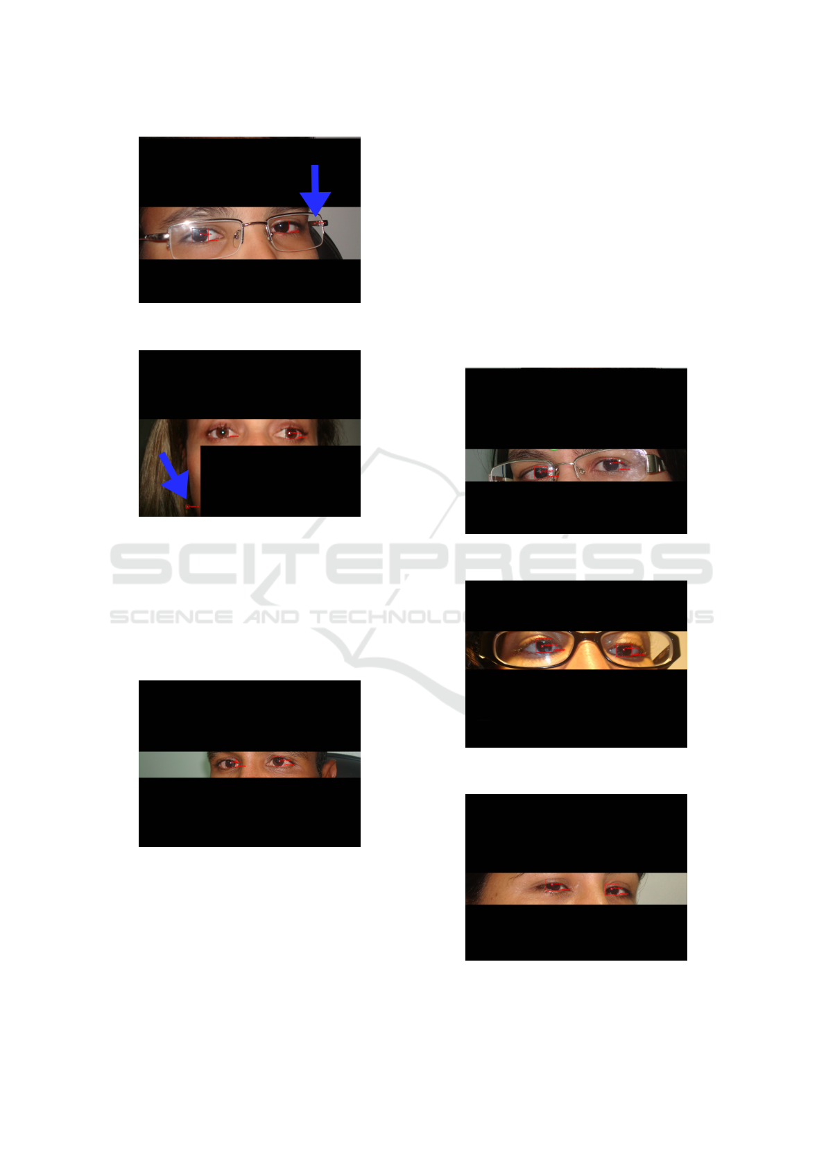
Figure 13: Patient 036 with wrong bright spot detection de-
noted by the blue arrow.
Figure 14: Patient 003 in INFRA position, where the blue
arrow denotes where the model detected the CR.
ror of 60∆ in horizontal measurements and 1∆ in ver-
tical measurements. Figure 16 shows patient 025 in
the LEVO position and a lateral occlusion of the lim-
bus; although the network precisely located the CR in
the image, it did not detect precisely the limbus, what
led to an error of 19 ∆ in horizontal measurements and
11∆ in vertical measurements.
Figure 15: Patient 009 in the LEVO position, with the lim-
bus laterally occluded.
The partial vertical occlusion of the limbus by the
eyelids also contributed to some error cases. Fig-
ure 17 illustrates such case., where patient 013 in the
LEVO position had an error of 43∆ in horizontal mea-
surements and 11∆ in vertical measurements. Figure
18 showcases patient 040 in the DEXTRO position,
eyelids vertically occluding the limbus with 26 ∆ of
error in horizontal measurements and 2∆ of error in
vertical measurements. Such errors occur most often
in the SUPRA and INFRA positions, but not exclu-
sively.
4.4 Discussion
In this work, we conducted tests to evaluate the
CNN’s capability to detect custom objects, specif-
ically the limbus and CR, and to measure strabis-
mus based on these detections. Both training phases
achieved significant results, particularly the second
phase, which utilized 5-fold cross-validation and
Figure 16: Patient 025 in the LEVO position, with the lim-
bus laterally occluded.
Figure 17: Patient 013 in the INFRA position, with the lim-
bus vertically occluded.
Figure 18: Patient 040 in the DEXTRO position, with the
limbus vertically occluded.
Cost-Effective Strabismus Measurement with Deep Learning
601

achieved an average F1-Score of 0.961. These results
highlight the potential for precise object detection.
When we compare our method to related works,
we observe significant improvements. In (Almeida,
2015) and (de Almeida et al., 2012), researchers re-
port that their methods are computationally expensive
due to the application of several image processing al-
gorithms. They also struggle with inaccuracies, such
as a doctor’s finger inadvertently appearing on the
patient’s face or other artifacts in the surroundings,
complicating the precise location of the face or eyes.
These issues make their methodologies less suitable
for real-world scenarios despite reporting average er-
rors of 5.6∆ for horizontal measurements and 3.83∆
for vertical measurements. In contrast, our proposed
method demonstrates excellent resistance to environ-
mental changes, blurriness, and other artifacts on the
patient’s face, as shown in Section 4.2.
Alternatively, (Dericio
˘
glu and C¸ erman, 2019)
aimed at using a mobile application to increase mea-
surement precision by delimiting the limbus and CR
with the help of a user interface. Such a method is sus-
ceptible to human error, along with being consider-
ably slower than the present method, requiring a man-
ual delimitation of the CR and the limbus, whilst our
method requires about 200ms to 500ms for each half
of the image to be processed by the YOLOv8 model.
(Cheng et al., 2021) used undisclosed image pro-
cessing algorithms to detect the limbus and the CR,
but such algorithms suffer from the same problems
that the work of (Almeida, 2015) suffers, that is, in-
ferior speed and much higher parametrization when
compared to a CNN-based approach.
The method implemented by (S¸
¨
ukr
¨
u Karaaslan
et al., 2023) utilizes the Mediapipe model, as ex-
plained in Section 2, to detect the pupil rather than
the limbus, aiming for more precise detection. How-
ever, detecting the pupil proves challenging due to
its small size, which limits the method’s applicabil-
ity in real-world scenarios where patients may be at
varying distances from the camera. In contrast, the
current work remains robust since it effectively ac-
commodates non-standardized imaging distances, al-
lowing the model to perform well under these condi-
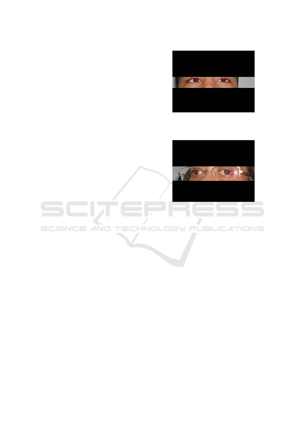
tions. Figures 19 and 20 illustrate challenging mea-
surements where the model achieves low error rates.
The tests demonstrated the model’s potential for
real-world application of strabismus measurement,
given the high agreement between the method’s and
strabologist’s measurements (see Figure 11 and Table
3). Despite the promising results, the model did not
perform well in certain adverse situations, as noted in
Section 4.3. The CR was the main obstacle to better
results, usually due to unwanted bright spots in the
Figure 19: Patient 033 in the INFRA position with 6∆ and
3∆ of error in horizontal and vertical measurements, respec-
tively. Vertically occluded limbus did not affect the final
measurement.
Figure 20: Patient 020 in the LEVO position with 0∆ and
5∆ of error in horizontal and vertical measurements, respec-
tively. The bright spots in the patient’s corrective lenses did
not affect the final detection.
corrective lenses of the patients or wrong detection of
the CR in distant locations of the image. Overall, re-
sults show a good potential for using the method in
real-world scenarios.
5 CONCLUSION
This work tackles the challenges of automated stra-
bismus measurement using the Hirschberg Test by
employing a cost-effective methodology, mainly de-
signed for resource-constrained environments and uti-
lizing deep learning techniques.
Through statistical analysis, we validated our
CNN-based strabismus measurement technique and
established meaningful metrics, including Mean Ab-
solute Error, Standard Deviation, and Pearson’s corre-
lation coefficient. Our results show that this method-
ology could serve as a preliminary tool for measuring
strabismus in resource-limited settings, such as rural
clinics or facilities lacking specialized equipment.
When analyzing the filtered results, the method
demonstrated error rates below the accepted threshold
of 10∆ for specialist measurements in the Hirschberg
ICEIS 2025 - 27th International Conference on Enterprise Information Systems
602

Test. However, it faced challenges with certain
blurred images and patients wearing corrective lenses.
These issues are expected, as the CNN identifies the
most likely locations for the CR point, and the fil-
tering process may not always correct inaccurate de-
tections. Additionally, there were difficulties related
to horizontally or vertically occluded limbus, which
are common error cases. The CNN struggles to ac-
curately estimate the location and size of the limbus
bounding box when it lacks relevant information in
the image. Nevertheless, the method is expected to
yield lower error rates for these situations. Such limi-
tations could be addressed by utilizing a larger dataset
and training for more epochs.
A possible use case for this method involves cap-
turing patients’ photos with a camera’s flash from dif-
ferent positions and then analyzing the images with
the model for preliminary strabismus measurement.
If the detection exceeds a threshold, the model could
prompt the patient to see an expert for in-person mea-
surements. This technique could help prevent many
cases of early strabismus, amblyopia, and other vi-
sion problems related to strabismus by providing oph-
thalmologists with a preliminary screening tool that
doesn’t require specialized equipment.
In future work, the bounding box filtering could
be augmented since it is a heuristic that does not al-
ways produce precise results. This is evident from
some detections of CR that are very distant (Euclidean
distance > 200px) in the image. A possible aug-
mentation for the bounding box filtering would be to
somehow segment the patient’s face and only consider
bounding boxes within that area.
Additionally, the training process could be opti-
mized by training for more epochs, fine-tuning hy-
perparameters (Tuba et al., 2021), or using a larger
dataset, which could enhance the CNN’s generaliza-
tion and object detection performance. Moreover,
case studies similar to (Cheng et al., 2021) could
be undertaken to evaluate the method’s effectiveness
and performance in clinics, particularly in challeng-
ing cases with real personnel.
ACKNOWLEDGEMENTS
The authors acknowledge the Coordenac¸
˜
ao de
Aperfeic¸oamento de Pessoal de N
´
ıvel Superior
(CAPES), Brazil - Finance Code 001, Conselho
Nacional de Desenvolvimento Cient
´
ıfico e Tec-
nol
´
ogico (CNPq), Brazil, and Fundac¸
˜
ao de Am-
paro
`
a Pesquisa Desenvolvimento Cient
´
ıfico e Tec-
nol
´
ogico do Maranh
˜
ao (FAPEMA) (Brazil), Empresa
Brasileira de Servic¸os Hospitalares (Ebserh) Brazil
(Grant number 409593/2021-4) for the financial sup-
port.
REFERENCES
Almeida, J.D. S., S. A. T. J. (2015). Computer-aided
methodology for syndromic strabismus diagnosis.
Journal of Digital Imaging, 28:462—-473.
Bazarevsky, V., Kartynnik, Y., Vakunov, A., Raveendran,
K., and Grundmann, M. (2019). Blazeface: Sub-
millisecond neural face detection on mobile gpus.
Buffenn, A. N. (2021). The impact of strabismus on psy-
chosocial heath and quality of life: a systematic re-
view. Survey of Ophthalmology, 66(6):1051–1064.
Canny, J. (1986). A computational approach to edge de-
tection. IEEE Transactions on pattern analysis and
machine intelligence, (6):679–698.
Cheng, W., Lynn, M. H., Pundlik, S., Almeida, C., Luo, G.,
and Houston, K. (2021). A smartphone ocular align-
ment measurement app in school screening for stra-
bismus. BMC ophthalmology, 21:1–10.
Choi, R. Y. and Kushner, B. J. (1998). The accuracy of
experienced strabismologists using the hirschberg and
krimsky tests. Ophthalmology, 105 7:1301–6.
de Almeida, J. D. S., Silva, A. C., de Paiva, A. C., and
Teixeira, J. A. M. (2012). Computational methodol-
ogy for automatic detection of strabismus in digital
images through hirschberg test. Computers in biology
and medicine, 42(1):135–146.
Dericio
˘
glu, V. and C¸ erman, E. (2019). Quantitative mea-
surement of horizontal strabismus with digital photog-
raphy. Journal of American Association for Pediatric
Ophthalmology and Strabismus, 23(1):18.e1–18.e6.
Durajczyk, M., Grudzi
´
nska, E., and Modrzejewska, M.
(2023). Present knowledge of modern technology and
virtual computer reality to assess the angle of strabis-
mus. Klinika Oczna / Acta Ophthalmologica Polonica,
125(1):13–16.
Google (2023). Google colaboratory. https://colab.research.
google.com/. Accessed: 2024-12-30.
Hashemi, H., Pakzad, R., Heydarian, S., Yekta, A.,
Aghamirsalim, M., Shokrollahzadeh, F., Khoshhal, F.,
Pakbin, M., Ramin, S., and Khabazkhoob, M. (2019).
Global and regional prevalence of strabismus: a com-
prehensive systematic review and meta-analysis. Stra-
bismus, 27:54 – 65.
Jocher, G., Chaurasia, A., and Qiu, J. (2023). Ultralytics
yolov8. https://github.com/ultralytics/ultralytics.
Khng, C. and Osher, R. H. (2008). Evaluation of the rela-
tionship between corneal diameter and lens diameter.
Journal of cataract and refractive surgery, 34.
Kirillov, A., Mintun, E., Ravi, N., Mao, H., Rolland, C.,
Gustafson, L., Xiao, T., Whitehead, S., Berg, A. C.,
Lo, W.-Y., Doll
´
ar, P., and Girshick, R. (2023). Seg-
ment anything.
Li, Z., Liu, F., Yang, W., Peng, S., and Zhou, J. (2022).
A survey of convolutional neural networks: Anal-
ysis, applications, and prospects. IEEE Transac-
Cost-Effective Strabismus Measurement with Deep Learning
603

tions on Neural Networks and Learning Systems,
33(12):6999–7019.
Lin, T., Maire, M., Belongie, S. J., Bourdev, L. D., Girshick,
R. B., Hays, J., Perona, P., Ramanan, D., Doll
´
ar, P.,
and Zitnick, C. L. (2014). Microsoft COCO: common
objects in context. CoRR, abs/1405.0312.
Miao, Y., Jeon, J. Y., Park, G., Park, S. W., and Heo, H.
(2020). Virtual reality-based measurement of ocular
deviation in strabismus. Computer Methods and Pro-
grams in Biomedicine, 185:105132.
O’Mahony, N., Campbell, S., Carvalho, A., Harapanahalli,
S., Hernandez, G. V., Krpalkova, L., Riordan, D.,
and Walsh, J. (2020). Deep learning vs. traditional
computer vision. In Advances in Computer Vision:
Proceedings of the 2019 Computer Vision Conference
(CVC), Volume 1 1, pages 128–144. Springer.
Petrou, M. and Bosdogianni, P. (1999). Image Processing:
The Fundamentals. John Wiley & Sons, Inc., USA,
1st edition.
Pundlik, S., Tomasi, M., Liu, R., Houston, K., and Luo, G.
(2019). Development and preliminary evaluation of a
smartphone app for measuring eye alignment. Trans-
lational Vision Science & Technology, 8(1):19–19.
Redmon, J., Divvala, S. K., Girshick, R. B., and Farhadi, A.
(2015). You only look once: Unified, real-time object
detection. CoRR, abs/1506.02640.
Refaeilzadeh, P., Tang, L., and Liu, H. (2009). Cross-
Validation, pages 532–538. Springer US, Boston,
MA.
Schwartz, G. (2006). The Eye Exam: A Complete Guide.
SLACK.
Tan, M. and Le, Q. V. (2019). Efficientnet: Rethink-
ing model scaling for convolutional neural networks.
CoRR, abs/1905.11946.
Tanabe, R. and Fukunaga, A. S. (2014). Improving the
search performance of shade using linear population
size reduction. In 2014 IEEE Congress on Evolution-
ary Computation (CEC), pages 1658–1665.
Tuba, E., Bacanin, N., Strumberger, I., and Tuba, M.
(2021). Convolutional Neural Networks Hyperparam-
eters Tuning, pages 65–84.
Valente, T. L. A., de Almeida, J. D. S., Silva, A. C., Teixeira,
J. A. M., and Gattass, M. (2017). Automatic diagno-
sis of strabismus in digital videos through cover test.
Computer Methods and Programs in Biomedicine,
140:295–305.
Van Thieu, N. and Mirjalili, S. (2023). Mealpy: An open-
source library for latest meta-heuristic algorithms in
python. Journal of Systems Architecture.
Varghese, R. and M., S. (2024). Yolov8: A novel object
detection algorithm with enhanced performance and
robustness. In 2024 International Conference on Ad-
vances in Data Engineering and Intelligent Comput-
ing Systems (ADICS), pages 1–6.
Zhuang, F., Qi, Z., Duan, K., Xi, D., Zhu, Y., Zhu, H.,
Xiong, H., and He, Q. (2019). A comprehensive sur-
vey on transfer learning. CoRR, abs/1911.02685.
S¸
¨
ukr
¨
u Karaaslan, Kobat, S. G., and Gedikpınar, M. (2023).
A new method based on deep learning and image pro-
cessing for detection of strabismus with the hirschberg
test. Photodiagnosis and Photodynamic Therapy,
44:103805.
ICEIS 2025 - 27th International Conference on Enterprise Information Systems
604