Exploring the Role of Brownian Motion in Financial Modeling: A

Stochastic Approach to the Black-Scholes Model for European Call

Options

Mehul Zawar

Independent Researcher, U.S.A.

Keywords: Financial Derivatives, Black Scholes, Geometric Brownian Motion, Stochastic Differential Equations, Option

Pricing, Euler-Maruyama Method, Sensitivity Analysis.

Abstract: Stochastic processes, particularly Brownian motion, have become foundational tools in financial modeling,

enabling the development of more accurate and insightful representations of market behavior. This paper

delves into the mathematical framework behind stochastic differential equations (SDEs) and their critical role

in the Black-Scholes model, specifically focusing on its application to European call options. We explore the

influence of key parameters, such as stock drift, volatility, and risk-free interest rate, on option pricing by

incorporating Brownian motion (Wiener processes) into the model. Through this exploration, we provide a

detailed analysis of how these stochastic components shape the dynamics of stock prices and the option's

value over time. The stability of the Black-Scholes model is evaluated under various boundary conditions,

revealing its robustness in financial modeling. However, limitations of the Black-Scholes approach, including

assumptions regarding constant volatility and market efficiency, are discussed, and potential improvements

are suggested. This paper underscores the significance of stochastic integration methods, including the Ito and

Stratonovich calculus, in refining the modeling of financial systems, thereby offering a comprehensive

understanding of the Black-Scholes framework's applicability and areas for enhancement.

1 INTRODUCTION

For a really long time, mathematics has been well

established in deterministic standards, underlining

amounts and frameworks that are represented by

fixed, unsurprising, and definitively characterized

connections. Deterministic frameworks, by their

actual nature, give obvious results while the

overseeing conditions and beginning circumstances

are known, practically ruling out vulnerability. Old-

style mechanics, for instance, works inside this

structure, offering definite answers for frameworks

like planetary movement or pendulum motions. In

any case, as the extent of math has extended to

address progressively complex peculiarities, it has

become apparent that some genuine frameworks do

not adjust to deterministic standards. All things being

equal, they display components of arbitrariness and

capriciousness, requiring the improvement of elective

systems for their investigation.

https://orcid.org/0009-0001-2848-2318

Haphazardness, in this specific situation, alludes

to the inborn vulnerability or fluctuation in results

that cannot not entirely settled ahead of time. Unlike

deterministic amounts, which are fixed and particular,

irregular amounts incorporate a scope of possible

results, each related with a specific probability or

likelihood. To address this, the likelihood hypothesis

has emerged as a central device for considering and

measuring irregularity. By doling out probabilities to

various results, we can develop numerical models that

catch the basic vulnerability while safeguarding the

design important for a thorough examination.

At the core of likelihood hypothesis lies the idea

of an irregular variable, which fills in as a numerical

deliberation for arbitrary amounts. An irregular

variable addresses a result of an irregular peculiarity

and is characterized as far as a likelihood dispersion

that depicts the probability of various qualities. This

reflection empowers us to dissect irregular

peculiarities, decreasing their intricacy by efficiently

planning them onto an organized structure. All

Zawar, M.

Exploring the Role of Brownian Motion in Financial Modeling: A Stochastic Approach to the Black-Scholes Model for European Call Options.

DOI: 10.5220/0013446300003956

Paper published under CC license (CC BY-NC-ND 4.0)

In Proceedings of the 7th International Conference on Finance, Economics, Management and IT Business (FEMIB 2025), pages 90-104

ISBN: 978-989-758-748-1; ISSN: 2184-5891

potential results for an irregular variable are held

inside an expert set known as the example space,

represented by Ω. The example space addresses the

universe of every possible result, and subsets of Ω

address occasions whose probabilities can be

investigated.

Regardless of the polish and force of this

structure, assigning probabilities to subsets of the

example space A ⊆ Ω is not always direct. For limited

example spaces, likelihood tasks can frequently be

instinctive or clear, especially when results are

similarly possible. However, as we move into

boundless or uncountable example spaces, the

method involved with relegating probabilities turns

out to be altogether really testing, frequently

requiring modern numerical instruments like the

measure hypothesis. At times, appointing

probabilities to all potential subsets of Ω might try to

be unimaginable, mirroring the inborn impediments

of our numerical apparatuses even with specific

intricacies.

By the by, the probabilistic structure gives a

passage to demonstrating dynamic frameworks

impacted by irregularity using stochastic cycles. A

stochastic cycle is an assortment of irregular factors

listed by time (or another boundary) that catches the

development of a framework under irregular impacts.

These cycles act as strong models for peculiarities

that unfurl over the long run, where results out of the

blue are affected by deterministic principles as well

as by arbitrary occasions or vacillations.

The utility of stochastic cycles reaches out across

a large number of disciplines, from physical science

and science to designing and financial matters. In

monetary math, for example, stochastic cycles have

upset the manner in which we comprehend and

anticipate market conduct. The monetary business

sectors are portrayed by a transaction of various

flighty elements, including the way the financial

backer behaves, macroeconomic patterns, and

external shocks. Conventional deterministic models

neglect to catch this intricacy, prompting the wide and

wide reception of stochastic methodologies. One of

the most compelling uses of stochastic cycles in

finance is the black Scholes model, which gives a

system to esteeming choices and different

subordinates. By integrating irregularity into the

display system, the Black Scholes model offers bits

of knowledge about the apparently tumultuous

developments of resource costs, empowering a better

dynamic despite vulnerability.

This paper centers on the meaning of stochastic

cycles in understanding and displaying frameworks

that challenge deterministic portrayal. While

stochastic models familiarize them with contrasted

and deterministic extra intricacy, their capacity to

catch the intrinsic irregularity of some certifiable

frameworks makes them imperative. It is vital to

recognize, in any case, that stochastic models are not

faultless. They are approximations that depend on

suspicions about the fundamental arbitrariness, and

their exactness is dependent on the legitimacy of

these presumptions. However, their prescient power

and capacity to give significant experiences

frequently outperform those of absolutely

deterministic models.

The essential target of this work is to dig into the

hypothetical underpinnings and common-sense uses

of stochastic cycles, with a specific accentuation on

their part in monetary demonstrating. By

investigating their numerical establishments and

showing their materiality to true situations, we plan

to feature the flexibility and force of stochastic cycles

as an instrument for grasping perplexing, unsure

frameworks. Through this conversation, we try to

delineate how the idea of irregularity, a long way

from being a constraint, can be tackled to make

models that enlighten the unpredictable elements of

the frameworks they address.

In the segments that follow, we will give a

complete outline of stochastic cycles, starting with

their hypothetical premise and continuing to their

applications in finance and then some unique

consideration will be given to the difficulties and

restrictions related with stochastic demonstrating, as

well as the systems used to defeat them. Toward the

end of this paper, we expect to show not just the

significance of stochastic cycles in present-day math

and science but additionally their significant effect on

our capacity to explore and get a handle on a world

formed by vulnerability.

2 STOCHASTIC PROCESSES

Stochastic cycles are numerical models that portray

frameworks which develop over the long run in an

irregular way. These cycles address the development

of a framework with irregular factors that change as

per probabilistic guidelines as opposed to

deterministic regulations. In contrast to deterministic

cycles, like those demonstrated by standard

differential conditions (Tributes), where the future

condition of the framework is not entirely set in stone

by its underlying circumstances, stochastic cycles

present a degree of vulnerability and irregularity. This

implies that even with known starting circumstances,

the future direction of the framework can follow

Exploring the Role of Brownian Motion in Financial Modeling: A Stochastic Approach to the Black-Scholes Model for European Call

Options

different ways, and there might be an endless number

of possible developments. Stochastic differential

conditions (SDEs) are normally used to show such

frameworks and are broadly material across different

fields, including physical science, science, financial

matters, and money.

Specifically, stochastic cycles are essential in

applications like subatomic movement (where

particles move haphazardly), meteorological

information (which shows eccentric varieties),

correspondence frameworks with clamor (where

signs are contorted by irregular obstruction),

populace hereditary qualities (where the hereditary

creation of a populace develops haphazardly over

ages), and monetary displaying (where resource costs

change haphazardly over the long run). In this large

number of cases, stochastic cycles give a structure to

demonstrating and grasping the innate haphazardness

and vulnerability in the frameworks.

2.1 Brownian Motion

Perhaps of the most widely utilized stochastic cycles,

particularly in monetary demonstrating, is the

Brownian movement. This cycle was first depicted by

the botanist Robert Brown in 1827, who noticed the

arbitrary movement of dust grains suspended in

water. Nevertheless, the numerical plan of the

Brownian movement was grown autonomously by

Albert Einstein in 1905 and Marian Smoluchowski in

1906. Brownian movement, likewise alluded to as a

Wiener interaction, is a ceaseless-time stochastic

cycle portrayed by irregular developments that are

regularly conveyed and display no anticipated

example.

In its most straightforward structure, Brownian

movement is displayed by an irregular variable W(t)

that relies consistently upon time t. The irregular

variable W(t) addresses the place of a molecule at

time t and is ordinarily expected to have the following

properties:

• W (0) = 0, meaning the interaction begins at

nothing.

• The cycle has free additions, which implies that

the value of W(t) at time t depends on the

ongoing time, rather than the previous history of

the interaction.

• The augmentations W(t) - W(s) are regularly

distributed with mean 0 and difference t - s,

where t > s.

• The way of the interaction is nonstop; however,

it is not differentiable from the other place,

which means that it shows an unpredictable and

inconsistent way of behavior.

The standard Brownian movement can be

discretized for computational purposes. A discretized

rendition is given by:

𝑊



(

𝑡

)

√

𝑡

∑

𝑋







√

𝑛𝑡



(1)

where 𝑋



are free irregular factors drawn from a

standard typical circulation, and t addresses time.

This discretization takes into account simpler

reproduction and mathematical investigation of the

interaction.

In monetary models, for example, the Black

Scholes model, Brownian movement fills in as an

essential structure block. In demonstrating stock

costs, Brownian movement is normally stretched out

to incorporate a float term, which addresses the

normal pace of return of the resource, and an

volatility term, which catches the vulnerability in the

cost changes. This is known as Geometric Brownian

movement (GBM) and is given by:

𝑋



=𝑒







(2)

where σ is the volatility of the resource, μ is the

float rate, and 𝑊



is the Brownian movement. The

Geometric Brownian movement models the irregular

stroll of stock costs and fills in as the reason for the

black Scholes condition.

In the black Scholes system, the stochastic

differential condition (SDE) overseeing the

advancement of resource costs is given by:

𝑑𝑋



=μ𝑋



𝑑𝑡 + σ𝑋



𝑑𝑊



(3)

where μ is the float, σ is the volatility, and 𝑊



addresses the standard Brownian movement. This

SDE shows how the stock cost develops in the long

run, with both deterministic and irregular parts that

impact the cost elements.

The discretized Brownian movement considers

representation of the apparently arbitrary way of

behaving of the cycle. The graphical portrayal of

Brownian movement, as displayed in Figure 1,

represents its inconsistent, erratic way. The

reproduction shows the way that the resource cost,

when demonstrated by Brownian movement, can

display sharp vacillations, expanding or diminishing

with no perceivable example.

FEMIB 2025 - 7th International Conference on Finance, Economics, Management and IT Business

Figure 1: Discretized Brownian way from BPATH1.m.

2.2 Stochastic Integration

Stochastic mix is a vital method utilized in the

examination of stochastic cycles. Given the arbitrary

idea of these frameworks, customary deterministic

reconciliation strategies, such as those in light of the

traditional Riemann basic, are not appropriate. All

things being equal, stochastic integrals are utilized to

represent the haphazardness and the intrinsic

flightiness of the cycles. Two normal types of

stochastic joining are 𝐼𝑡𝑜 and Stratonovich integrals,

each with its own arrangement of rules and

applications.

The 𝐼𝑡𝑜 basic is the most widely involved method

in stochastic mathematics. It depends on the

understanding that the integrand is assessed at the

left-hand end point of the time increase. The 𝐼𝑡𝑜 basic

for a capability ℎ

(

𝑡

)

more than a period span



0,𝑇



given by

ℎ

(

𝑡

)

𝑑𝑡





=ℎ𝑡







𝑊𝑡









−𝑊𝑡







(𝐼𝑡𝑜)



(4)

This detail is frequently utilized while working

with stochastic cycles in finance, as it accurately

catches the way of acting of irregular frameworks

over the long haul.

Then again, the Stratonovich vital is somewhat

divergent in that it assesses the integrand at the

midpoint of each time increase. This vital is many

times utilized in actual applications where the

understanding of the cycle requires such a definition.

The Stratonovich basic for a capability ℎ

(

𝑡

)

is given

by:

ℎ

(

𝑡

)





𝑑𝑡=ℎ

𝑡



+𝑡











𝑊𝑡



−𝑊𝑡







(Stratonovich).

(5)

While the Stratonovich basic can be more precise

in specific situations, the 𝐼𝑡𝑜 essential remaining

parts the norm for most monetary applications

because of its numerical properties and

straightforwardness in calculation.

2.3 The Euler-Maruyama Method

The Euler-Maruyama strategy is a mathematical

procedure used to settle stochastic differential

conditions (SDEs), especially for independent SDEs

of the structure:

𝑑𝑋

(

𝑡

)

𝑓

𝑋

(

𝑡

)

𝑑𝑡

+𝑔𝑋

(

𝑡

)

𝑑𝑊

(

𝑡

)

,with 𝑋

(

)

=𝑋



(6)

This strategy is a characteristic expansion of the

traditional Euler technique, which is utilized to tackle

customary differential conditions (tribulations), and it

adjusts it to the stochastic case. The Euler-Maruyama

technique approximates the arrangement by

discretizing the time spans and refreshing the state at

each time step. The strategy is especially helpful

when an insightful answer for the SDE is difficult to

acquire.

When applied to the SDE administering the Black

Scholes model, the Euler-Maruyama strategy yields

the accompanying estimate:

𝑋

(

𝑡



)

=𝑋

(

𝑡



)

+𝜇𝑋

(

𝑡



)

Δ𝑡

+𝜎𝑋

(

𝑡



)

Δ𝑊



(7)

where Δ𝑡 is the time step, and Δ𝑊



is the adjustment

of the Brownian movement over the stretch.

The Euler-Maruyama technique is in many cases

utilized in computational money to mathematically

tackle the Black Scholes PDE and different models

including stochastic cycles. It gives an effective and

somewhat straightforward method for recreating the

arbitrary elements of resource costs and other

monetary factors. Nonetheless, while it is not difficult

to carry out, it may not generally be the most reliable

strategy, particularly while managing exceptionally

nonlinear frameworks or tiny time steps.

By applying the Euler-Maruyama technique to the

stochastic differential conditions, it is feasible to

determine the Black Scholes halfway differential

Exploring the Role of Brownian Motion in Financial Modeling: A Stochastic Approach to the Black-Scholes Model for European Call

Options

condition (PDE), which is integral to choice

estimating and monetary demonstrating. This PDE

takes into account the calculation of the cost of a

choice given different boundaries like the stock cost,

volatility, time to development, and loan fee. The

capacity to tackle this PDE mathematically through

techniques like Euler-Maruyama empowers experts

to precisely demonstrate and cost monetary

subordinates more.

3 THE BLACK SCHOLES

FRACTIONAL DIFFERENTIAL

CONDITION

DEMONSTRATING SYSTEM

The Black Scholes structure addresses a huge

achievement in the demonstration of monetary

business sectors, giving a precise method for

anticipating the worth of a portfolio or monetary

resources over the long run. At its center, the Black

Scholes framework tries to depict the value elements

of portfolios comprising a mix of bonds and stocks.

Securities, being less unpredictable, give a steady part

to the portfolio, while stocks contribute a level of

haphazardness because of market vacillations. By

tending to both these resource classes inside a bound

together system, the Black-Scholes model has turned

into a foundation of current monetary math.

A few systems exist under the Black Scholes

structure, the most unmistakable being the European

and American Call Cost choices. These choices

contrast in their standards for practicing the

agreement, with European choices allowing exercise

just at termination and American choices permitting

exercise anytime before expiry. In spite of this

differentiation, both depend on the stochastic course

of Geometric Brownian movement to show resource

cost conduct. Geometric Brownian movement is a

consistent time process generally used to depict the

irregular developments of stock costs, and it shapes

the numerical spine of the Black Scholes model.

To determine the Black-Scholes condition, a few

key suspicions are made about the way of behaving

of the market and the properties of the resources in

question. These suspicions, which improve the

hidden science while safeguarding the model's utility,

are as per the following:

1) The cost of the hidden resource follows a

Geometric Brownian movement.

2) Bonds and stocks can be traded continuously in

time, considering Δ𝑡 to change without a hitch

and empowering continuous changes according

to the portfolio.

3) The subordinate of the portfolio esteem to the

cost of the stock,





, is a smooth capability, and

fragmentary portions of the stock can be traded

without limitation.

4) The adjustment of portfolio esteem is affected

simply by the varieties in 𝑉 (the portfolio

esteem) and 𝑆 (the stock cost), barring any

conditional expenses or charges related with the

trading of resources.

5) There are no limitations on trading resources; all

resources can be exchanged unreservedly

whenever.

3.1 Basic Black Scholes Model

The Black Scholes model can be refined into a

worked on structure that is open even to those with

restricted insight in stochastic cycles or likelihood

hypothesis. This essential detailing spins around two

conditions got from Geometric Brownian movement

and three essential boundaries: stock volatility (σ),

stock float (μ), and the gamble free loan cost (𝑟).

These boundaries, when integrated into the

framework, yield the accompanying primary

conditions:

𝐵



=𝑒



(8)

𝑆



=𝑆



𝑒







(9)

Here, 𝐵



addresses the worth of the security at

time 𝑡, which develops deterministically at the free

rate of the gamble 𝑟, while 𝑆



signifies the cost of the

stock, which advances stochastically after some time,

impacted by the Wiener cycle 𝑊



Every boundary in these situations assumes a

pivotal part in significantly shaping the way of

behaving of the model:

• Sans risk loan fee ( 𝒓): This addresses a

hypothetical pace of profit from a venture

without any gamble of monetary misfortune,

working on the valuation of the bond part in the

portfolio.

• Stock Volatility (𝝈): This captures the size of

the variances in the long-term stock cost. Higher

volatility demonstrates a more notable

probability of huge cost changes.

• Stock Float (𝝁): This mirrors the typical rate of

return of the stock, addressing its general pattern

after some time.

FEMIB 2025 - 7th International Conference on Finance, Economics, Management and IT Business

The model is established in the idea of

martingales, a fundamental thought in the likelihood

hypothesis. Martingales are processes that address

fair games, where the normal future worth,

considering all previous data, approaches the ongoing

worth. With regard to the Black Scholes model,

martingales are utilized to determine a replication

procedure for portfolios, guaranteeing that they are

self-funding. A self-funding portfolio keeps up with

its worth without requiring extra capital after its

underlying speculation. Using likelihood

disseminations, especially the ordinary conveyance,

the Black Scholes model guarantees a numerically

reliable system for estimating subordinates.

Although incorporation of the two stocks and

bonds adds authenticity to the model, it additionally

presents intricacy, as the stochastic idea of stocks

communicates with the deterministic development of

securities. To zero in on the stochastic components,

this article works on the esteem of the bond, 𝐵



, to a

consistent of 1, reflecting the self-supporting property

of the portfolio. This rearrangement prompts the

stochastic differential condition:

𝑆



=𝑒

















(10)

where 𝑊





addresses a standard Wiener process.

Be that as it may, this condition, while

numerically sound, isn't the most commonsense

decision for the end goal of demonstrating. All things

considered, this paper takes on the European Call

Choice system, as itemized in Segment 3, involving

fundamental Brownian movement for

straightforwardness. The methodology is consistent

with that crafted by Higham, using his most

memorable Brownian movement code to successfully

display the black Scholes framework.

3.2 Non-Zero Revenue Rates

A significant element of the Black Scholes model is

its capacity to work under changing loan cost

conditions, including zero loan fees. Figure 2 shows

a situation where the gamble free rate 𝑟 is set to zero.

For this situation, the value of the bond remains

steady at 1, while the price of the stock changes due

to its volatility (σ) and drift (μ). For this exhibit, the

boundaries were set as follows: σ= 0.18, 𝑟 = 0,

μ= 0.15, 𝑆



=20, and 𝐾 = 25.

Figure 2: The Black Scholes Model using Brownian

Movement with Zero Interest.

Although the model requires zero loan costs, this

situation frequently needs authenticity in monetary

business sectors, where loan costs ordinarily impact

venture development. The consolidation of non-zero

loan fees presents more prominent dynamism and

reflects genuine circumstances all the more precisely.

For example, in forward agreements, where the

understanding includes selling the stock at a

foreordained value 𝐾 at time 𝑇, the shortfall of

interest leads to a distorted valuation. The forward

cost is given by 𝐾=𝑆



𝑒



. When 𝑟 = 0, this

relationship breaks down, highlighting the

importance of non-zero financing costs in a sensible

market demonstration.

By including non-zero loan fees, the model

catches the inflexible development of money after

some time. While this presents extra intricacy, it tends

to be overseen under fitting circumstances, yielding a

more exact and dynamic portrayal of the Black

Scholes framework.

4 THE BLACK SCHOLES

RECIPE FOR EUROPEAN

CALL VALUE OPTIONS

The European Call Choice gives a structure to

deciding the worth of a monetary agreement where

the trading of the basic resource or ware happens at a

foreordained future date. This differs from the

American Call Choice, where the holder has the

adaptability to execute the trade whenever previously

or on the lapse date. The American Call Choice, while

more flexible, presents a more elevated level of

intricacy to demonstrating, making it more

challenging for those new to the Black Scholes

Exploring the Role of Brownian Motion in Financial Modeling: A Stochastic Approach to the Black-Scholes Model for European Call

Options

system. Subsequently, for the motivations behind this

paper, the attention is still on the European Call

Choice because of its relatively easier numerical

design and the creator's ongoing degree of skill.

The recipe for the worth of the European Call

Choice can be communicated as:

𝑠Φ



𝑠

𝑘



+𝑟+



𝑇

√

𝑇



− 𝑘𝑒



Φ



𝑠

𝑘



+𝑟−



𝑇

√

𝑇



(11)

where, Φ

(

𝑥

)



√





𝑒









∞

𝑑𝑦

Here, (𝑉

(

𝑠,𝑇

)

) addresses the worth of the call

choice at time (𝑇), with (𝑠) being the ongoing cost of

the stock, (𝑘) as the strike cost of the choice, (𝑟) as

the free-loan gamble fee, (σ) as the volatility of the

stock, and (𝑇) as the opportunity to terminate. The

capability (Φ

(

𝑥

)

) is the total dispersion capability of

the standard ordinary dissemination.

This equation gives the hypothetical valuation of

the European Call Choice under the supposition that

the stock cost follows a Geometric Brownian

movement and that no profits are paid during the

existence of the choice. One basic element of this

model is the utilization of the combined typical

conveyance to compute probabilities related to the

resource cost coming to or surpassing the strike cost

by termination.

4.1 Adapting the Model with

Geometric Brownian Motion

In its standard structure, the Black Scholes recipe

accepts that the stock cost (𝑠) is steady for the period

displayed. While this is helpful for computing the

normal worth of a portfolio at a particular second in

time, it isn't great for additional unique situations

where stock costs change because of fundamental

market factors. To address this limit, the stock cost

(𝑠) was demonstrated as a stochastic cycle, explicitly

utilizing the Geometric Brownian movement.

This was accomplished by utilizing adjusted

Brownian movement calculations, adjusted from

Highman's primary work in stochastic demonstrating.

Beginning with Highman's unique code for

reproducing Brownian movement, a subsidiary

rendition was created to integrate the particular

boundaries and states of the Black Scholes model.

The revised code allowed the recreation of stock cost

ways after some time, considering variables such as

float, volatility, and the risk-free rate of return.

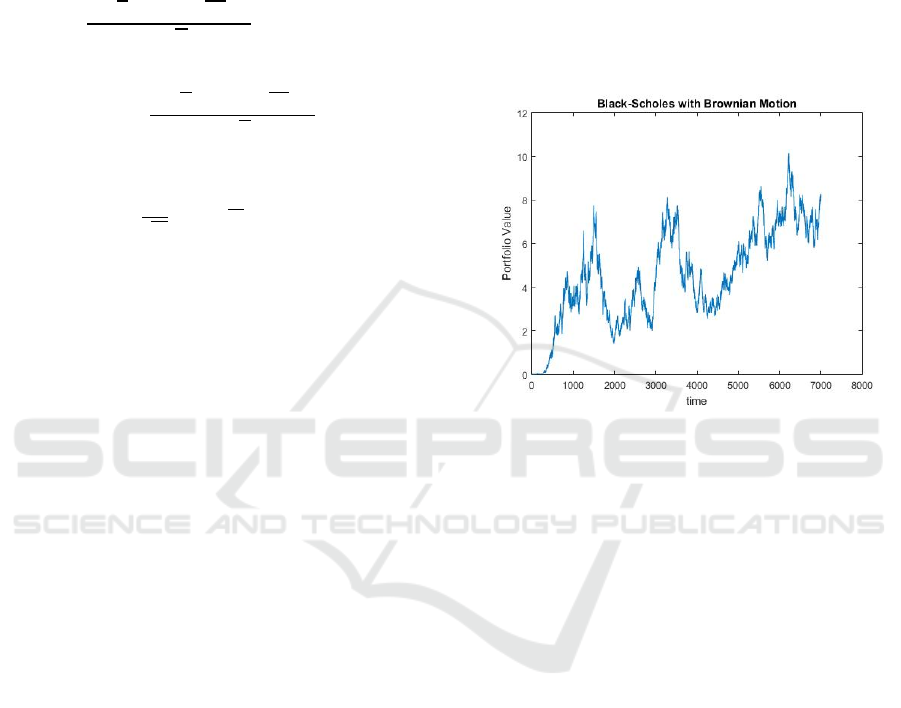
To show the viable use of this methodology, the

model was executed with the accompanying

boundaries: stock volatility (σ= 0.18), stock float

(μ= 0.15), non-risk loan fee (𝑟 = 0.06), time to

lapse (𝑇 = 7000), starting stock cost (𝑠



=20),

and strike cost (𝑘 = 25). The consequences of this

recreation are shown in Figure 3.

Figure 3: Test Black Scholes Recreation over the Long

Haul with Geometric Brownian Motion.

This figure shows the development of the stock

cost affected by Brownian movement and features the

stochastic idea of the cycle. The utilization of

Geometric Brownian movement permits the model to

catch the inborn arbitrariness of stock cost

developments while sticking to the requirements

forced by the black Scholes structure.

4.2 Insights from the Simulation

The mix of Geometric Brownian movement acquaints

us with a degree of authenticity with the model that is

missing, while expecting consistent stock costs. It

mirrors the volatility and float that stocks insight in

certifiable monetary business sectors, giving a more

powerful and reasonable portrayal of resource

conduct over the long run.

In any case, it is significant that this variation

requires computational apparatuses and calculations

fit for taking care of stochastic differential conditions

and reenacting huge quantities of potential stock cost

ways. The progress of such recreations additionally

depends on the precision of the information

boundaries, especially (σ), (μ), and (𝑟), as these

FEMIB 2025 - 7th International Conference on Finance, Economics, Management and IT Business

simply impact the anticipated directions of the stock

costs and, thusly, the valuation of the call choice.

By zeroing in on the European Call Choice and

utilizing Geometric Brownian movement, this paper

offers a primary yet strong investigation of the Black

Scholes system, preparing for future examinations to

consolidate further developed elements, for example,

exchange expenses, profits, and multi-resource

portfolios.

5 PARAMETER IMPACT

The Black Scholes model is affected by various key

boundaries, each of which assumes a basic role in

deciding the way of behaving and result of the model.

To more readily comprehend the individual and

joined impacts of these boundaries, a broad

investigation was directed. This examination plans to

measure the responsiveness of the model to changes

in three essential boundaries – risk free rate of return

(𝑟), stock volatility (σ), and stock float (μ) - while

keeping the different circumstances consistent.

To accomplish this, a progression of

reproductions was performed:

1) Single-Boundary Variation: For every

boundary, three models were controlled by

fluctuating the boundary, while the other two

were held steady. This approach confines the

impact of the boundary under scrutiny.

2) Combined Boundary Variation: Extra

preliminaries were led by fluctuating two

boundaries while keeping the third consistent.

This gives an understanding of the connection

and consolidated impact of these boundaries on

the model.

This segment presents the discoveries of these

tests, outlining the effect of every boundary on the

portfolio's worth as anticipated by the Black-Scholes

model.

5.1 Impact of Risk-Free Rate of Return

The risk-free rate of return (𝑟) is a boundary in the

black Scholes condition that addresses the

hypothetical return of a gamble-free venture. In

contrast to different boundaries, 𝑟 does not impact the

Brownian movement by administering stock cost

variances, yet it straightforwardly influences the

limiting of the strike cost in the black Scholes recipe.

For this examination, the volatility and floating

limits of the stocks were kept steady at σ= 0.18 and

μ= 0.15, individually. The advantages of 𝑟 differed

in three situations: the standard value 𝑟 = 0.06, the

expanded value 𝑟 = 0.09 and the decreased value

𝑟 = 0.03.

Figure 4: The Effect of Risk-Free Rate of Return on the

Black Scholes Model.

In Figure 4, the standard situation (𝑟 = 0.06) is

portrayed in blue, filling in as a kind of perspective

point. The situation with an expanded financing cost

(𝑟 = 0.09) is shown in red, while the situation with

a reduced loan fee (𝑟 = 0.03) is shown in green.

True to form, the portfolio esteem increases

marginally when 𝑟 is higher and decreases somewhat

when 𝑟 is lower. However, the general effect of 𝑟 on

portfolio esteem after some time is not significant.

The curves remain firmly adjusted, demonstrating

that while 𝑟 affects the limitation of the strike value,

its impact on the general portfolio is moderately little

contrasted with different boundaries. This proposes

that the risk-free rate of return is a less delicate

boundary in the Black Scholes model, especially

when contrasted with volatility and float.

5.2 Impact of Stock Volatility

Stock volatility (σ) is a basic boundary in the Black

Scholes model, as it straightforwardly influences both

the Brownian movement of the stock cost and the

fractional differential condition used to compute the

choice value. It evaluates the level of variety in the

stock value and is, subsequently, a proportion of

market vulnerability.

To avoid the impact of σ, the limit of stock float

and the cost of risk-free loans were kept steady at μ=

0.15 and 𝑟 = 0.06. The benchmark situation (σ=

0.18) was considered against two elective situations:

expanded volatility (σ= 0.27) and reduced volatility

(σ= 0.12).

Exploring the Role of Brownian Motion in Financial Modeling: A Stochastic Approach to the Black-Scholes Model for European Call

Options

Figure 5: The Effect of Stock Volatility on the Black

Scholes Model.

In Figure 5, the benchmark situation is shown in

blue, with expanded volatility represented in red and

diminished volatility in green. The outcomes uncover

that higher volatility at first seems to build the

portfolio's worth. However, over the natural course of

time, this impact decreases, and the time-consuming

development pace of the portfolio eases back. This is

logical because of the expanded vulnerability related

with greater volatility, which balances the momentary

additions.

On the other hand, lower volatility at first stifles

the portfolio's worth, yet after some time, the

development rate speeds up, prompting a higher-

esteemed portfolio in the long haul. This conduct

lines up with the idea that lower volatility diminishes

vulnerability, bringing about more steady and

unsurprising development.

5.3 Combined Boundary Effects

To comprehend the communication between

boundaries, additional reenactments were directed in

which two boundaries were changed at the same time

while the third was kept steady. The blends tried

were: 1. Fluctuating 𝑟 and σ while maintaining μ

consistency. 2. Fluctuating 𝑟 and μ while keeping σ

consistent. 3. Fluctuating σ and μ while holding 𝑟

consistent.

The results show that the association between σ

and μ affects the value of the portfolio. At the point

when the two boundaries are expanded, the portfolio

displays momentary additions because of the greater

float (μ), however, these increases are tempered by

the drawn-out impacts of expanded volatility ( σ).

However, decreasing the two boundaries brings about

a more steady, but slower developing portfolio.

The blend of 𝑟 and σ showed moderate impacts,

with changes in σ ruling the general way of behaving.

The connection among 𝑟 and μ was the most un-

effective, as 𝑟 principally influences the limiting

variable and doesn't straightforwardly impact the

stock cost elements.

5.4 Insights and Implications

This investigation features the changing levels of

responsiveness of the black Scholes model to its key

boundaries:

1) Risk Free Rate of Return ( 𝑟): A somewhat

minor impact, basically influencing the limiting

of the strike cost.

2) Stock Volatility (σ): A critical boundary that

impacts both the transient way of behavior and

the long-term development of the portfolio.

3) Stock float ( μ ): Assumes a crucial part in

deciding the development direction of the

portfolio, especially in mix with volatility.

Understanding these awarenesses takes into

consideration more educated decision-production

while applying the Black Scholes model to genuine

situations. For example, precisely assessing σ and μ

is basic for dependable choice valuing, while varieties

in 𝑟 can frequently be treated as an optional concern.

These discoveries likewise give an establishment

to future investigations to investigate extra factors,

for example, exchange expenses, profits, and multi-

resource portfolios, which could additionally refine

the prescient force of the Black Scholes structure.

6 STOCK FLOAT IMPACT

The last single boundary tested was the stock float

(μ), a key component in the demonstration of stock

costs. The floating boundary addresses the normal

rate of return of the stock and assumes a critical role

in the stochastic differential condition that oversees

the cost elements of the stock. Unlike Risk Free Rate

of Return (𝑟), which influences the limiting term in

the Black Scholes recipe, and volatility (σ), which

captures vulnerability, the floating boundary

straightforwardly impacts the deterministic part of the

direction of the stock cost through Brownian

movement.

To separate the effect of μ, the other two

boundaries were held consistent at 𝑟 = 0.06 and

σ= 0.18, while μ was differed. The gauge situation,

where μ= 0.15, was plotted in blue for reference.

FEMIB 2025 - 7th International Conference on Finance, Economics, Management and IT Business

Two extra situations were thought of: an expanded

float of μ= 0.20 and a decreased float of μ= 0.10.

The consequences of these reproductions are

portrayed in Figure 6.

Figure 6: The Effect of Stock Float on the Black Scholes

Model.

From Figure 6, it becomes obvious that the stock

float boundary significantly affects the portfolio's

worth, especially in the long haul. At the point when

the float was expanded to μ= 0.20, the portfolio's

worth developed fundamentally, unparalleled the ideal

forward agreement level of 𝑘 = 25 in a somewhat

brief period. This significant development shows the

immediate connection between the float rate and the

remarkable development capability of the portfolio.

On the other hand, when the float decreased to

μ= 0.10, the direction of development of the

portfolio was unfavorably affected. The last value of

the portfolio was roughly 50% of the value seen in the

benchmark situation, reflecting the discounted

commitment of the deterministic part of the cost of

the stock. This articulated lessening can be attributed

to the way that decreasing μ to 66% of its unique

value results in a noticeable decrease in the normal

pace of return. Interestingly, expanding μ by an

addition similar to 133% of its unique value enhances

the potential for development of the portfolio.

6.1 Short-Term sersus Long Haul

Effects

The effect of changes in the floating boundary is

contrastingly displayed throughout short- and long-

time skylines:

1) Short-Term Effects: temporarily, varieties in μ

may not essentially adjust the portfolio's worth

on the grounds that the impacts of float

compound after some time. This line up with the

stochastic idea of stock cost conduct, where the

Brownian movement part rules in the short run.

2) Long-term effects: Throughout longer time

spans, the deterministic part determined by μ

turns out to be progressively stronger, causing

significant disparity between the direction of

portfolios with various float rates. This makes

sense of why the portfolio with μ= 0.20

outflanked the benchmark and the decreased

float situation overwhelmingly.

6.2 Implications for Portfolio

Management

The examination shows the significance of precisely

assessing the float boundary while using the Black

Scholes model to portfolio the board and to estimate

the choice. Little changes in μ can cause enormous

contrasts in the results of the long-term portfolio,

highlighting the awareness of the model to this limit.

This is especially significant in situations including

long-dated choices or when the model is applied to

assess the development capacity of a portfolio

overstretched time spans.

Also, that's what the discoveries propose:

1) Expanded Float (𝜇): A higher float rate

improves the development capability of the

portfolio however may likewise mirror a higher

gamble climate, as stocks with higher expected

returns frequently accompany expanded

vulnerability.

2) Diminished Float (𝜇): A lower float rate brings

about more moderate development projections,

making it reasonable for risk-disinclined

financial backers. However, it also demonstrates

a decreased ability to achieve significant yields

in the long run.

6.3 Comparative Sensitivity

While contrasting the responsiveness of the Black

Scholes model to its three essential boundaries – Risk

Free Rate of Return (𝑟), stock volatility (σ), and stock

float (μ) — obviously μ applies a more critical impact

on the portfolio's worth, particularly over significant

stretches. Dissimilar to 𝑟, which has a minor effect,

and σ, which presents changeability, μ decides the

normal development rate, making it a basic boundary

for key navigation.

6.4 Future Considerations

Given the significant effect of μ on portfolio results,

future examinations could zero in on refining

Exploring the Role of Brownian Motion in Financial Modeling: A Stochastic Approach to the Black-Scholes Model for European Call

Options

strategies for assessing the float rate. Consolidating

variables like macroeconomic circumstances, area

explicit patterns, and authentic stock execution could

improve the precision of μ gauges. Moreover,

investigating the transaction among μ and different

boundaries, especially σ , may yield further

experiences into upgrading portfolio procedures

under shifting economic situations.

7 MIXED BOUNDARY IMPACT

In this part, we investigate the joined impacts of

fluctuating two boundaries all at once inside the

Black Scholes model to acquire further experiences

into the transaction and by and large effect of these

boundaries on the portfolio's way of behaving. By

leading assembled reenactments, each set of

boundaries was efficiently changed while keeping the

third boundary steady. This approach permits us to

more readily comprehend the connections between

these basic elements and their effect on the portfolio

esteem over the long run.

Likewise with the past single-boundary

reproductions, the standard situation — characterized

by μ= 0.15, σ= 0.18, and 𝑟 = 0.06 — is

addressed in blue for reference in all figures.

7.1 Volatility and Risk-Free Rate of

Return

The main gathering of reenactments zeroed in on the

joined effect of stock volatility (σ) and the risk-free

rate of return ( 𝑟), with the stock float (μ) held

consistent at 0.15. The accompanying situations were

investigated:

1) Both Boundaries Increased: Volatility was

expanded to σ= 0.23, and the loan fee was

raised to 𝑟 = 0.09. The results, as shown in

Figure 7, show that this situation at first creates

the most noteworthy portfolio esteem. However,

in the long run, the development rate moderates

and the last value becomes like a gauge.

2) Both Boundaries Decreased: Volatility was

diminished to σ= 0.12, and the loan cost was

brought down to 𝑟 = 0.05. At first, this design

causes the least portfolio esteem. Curiously, as

reproduction advances, the portfolio

accomplishes a higher last worth contrasted

with both the benchmark and the situation with

expanded boundaries.

3) One Boundary Expanded, the Other Decreased:

• Volatility expanded to σ= 0.20, and

loan cost diminished to 𝑟 = 0.02. This

situation, addressed in black, at first

outflanks the gauge at the end of the day

brings about the least portfolio worth of

the gathering.

• Volatility diminished to σ= 0.13, and

loan fee expanded to 𝑟 = 0.08. Plotted

in yellow, this design created the most

elevated last portfolio esteem in the

gathering.

Figure 7: The Blended Effect of Stock Volatility and Risk-

Free Rate of Return on the Black Scholes Model.

7.2 Risk-Free Rate of Return and

Stock Drift

The subsequent gathering inspected the consolidated

impacts of the risk-free rate of return (𝑟) and the stock

float (μ), keeping the volatility consistent with σ=

0.18. Reenactments revealed the accompanying

elements:

1) Both Boundaries Increased: Setting 𝑟 = 0.09

and μ= 0.20 brought about a fundamentally

higher portfolio esteem compared to the

standard. This development was dramatic, as

confirmed by the green direction in Figure 8.

2) Both Boundaries Decreased: Diminishing 𝑟 to

0.04 and μ to 0.09 delivered the most minimal

portfolio esteem overwhelmingly — roughly

33% of the pattern.

3) One Boundary Expanded, the Other Decreased:

• Expanding 𝑟 to 0.08 and diminishing 𝜇 to

0.10, plotted in black, brought about a lower

portfolio esteem. In any case, the higher

financing cost marginally relieved the decay

in contrast with the situation in which the

two boundaries were reduced.

FEMIB 2025 - 7th International Conference on Finance, Economics, Management and IT Business

100

• Expanding μ to 0.23 while diminishing 𝑟 to

0.02, plotted in yellow, yielded a last

portfolio esteem equivalent to the situation

where the two boundaries were expanded,

featuring the predominant impact of the

greater float.

Figure 8: The Blended Effect of Stock Float and Risk-Free

Rate of Return on the Black Scholes Model.

7.3 Stock Float and Volatility

In the last gathering, the risk-free rate of return was

held consistent at 𝑟 = 0.06, while the stock float (μ)

and volatility (σ) were shifted. The accompanying

situations are broken down:

1) Both Boundaries Increased: Expanding μ to

0.20 and σ to 0.24, as displayed in green in

Figure 9, brought about a reliably higher

portfolio esteem contrasted with the benchmark

all through the recreation.

2) Both limits reduced: Setting μ= 0.09 and σ=

0.12, plotted in red, prompted a reliably lower

portfolio esteem than the pattern.

3) One boundary expanded, the other decreased:

• The volatility expanded to σ= 0.21, and

float decreased to μ= 0.10, plotted in

black. At first, the portfolio esteem closely

followed the benchmark at the end of the day

and brought about the least last worth of the

gathering.

• Float expanded to μ= 0.23, and volatility

diminished to σ= 0.12, plotted in yellow.

This setup accomplished the most

noteworthy last portfolio esteem,

outflanking any remaining situations across

all gatherings.

Figure 9: The Blended Effect of Stock Float and Volatility

on the Black Scholes Model.

7.4 Parameter Effect Interpretation

By efficiently shifting two boundaries all at once, the

accompanying key connections were noticed:

1) The float of the stock (μ) and the risk-free

financing cost (𝑟) show a positive relationship,

with expansions in the two limits causing higher

portfolio values.

2) Stock volatility (σ) has a converse relationship

with both float and financing cost, where higher

volatility will in general hose portfolio

execution, especially when matched with lower

float or loan fees.

Among the boundaries, stock float (μ) arose as the

most compelling, probable because of its one of a

kind job in Geometric Brownian movement. risk-free

rate of return (𝑟), then again, made the most un-

articulated difference, as its impact is restricted to the

limiting term in the Black Scholes condition. Stock

volatility (σ), with its double job in both Geometric

Brownian movement and the Black Scholes PDE,

affected portfolio conduct.

7.5 Implications for Model Stability

The Black Scholes model the remaining parts are

straightly stable under fluctuating boundary blends.

Soundness is guaranteed by limit conditions applied

to the semi-discretized PDE administrator, as upheld

by existing writing (Hout,2012; Windcliff et al.,

2004). In particular, the second subsidiary of the

choice worth, 𝑉



, disappears as the basic resource

cost turns out to be enormous, guaranteeing that

boundary actuated development doesn't undermine

the model.

Exploring the Role of Brownian Motion in Financial Modeling: A Stochastic Approach to the Black-Scholes Model for European Call

Options

101

(

𝑥

)

√

2π

𝑒









𝑑𝑦



∞

(12)

This examination highlights the vigor of the Black

Scholes model while featuring the significance of

boundary determination in accomplishing precise

portfolio expectations and successful gamble the

board systems.

8 THE WEAKNESSES OF THE

BLACK-SCHOLES MODEL

The Black-Scholes model has many inherent

weaknesses, most notably due to the five fundamental

assumptions it makes to simplify the complex real-

world financial environment. These assumptions are

the foundation of the model, but they also

significantly limit its applicability in real-world

scenarios. The model assumes the following.

Although these assumptions allow the model to be

mathematically tractable and relatively easy to

implement, they also introduce significant

weaknesses. If any of these assumptions are violated

under real market conditions, the Black-Scholes

model becomes invalid, leading to inaccurate option

pricing and poor predictions for hedging strategies.

Let us examine each of these assumptions in more

detail and the corresponding weaknesses they

introduce.

1) Geometric Brownian Motion Assumption

and Constant Volatility Assumption. This

assumption states that the underlying asset

follows a random walk in the form of geometric

Brownian motion. However, real financial

markets do not always exhibit behavior

consistent with this assumption. Asset prices

often exhibit jumps or other forms of

noncontinuous movements that are not captured

by GBM. Furthermore, market conditions may

lead to volatility clustering, where periods of

high volatility are followed by more periods of

high volatility, and vice versa, which GBM

cannot account for. This can lead to inaccurate

predictions, particularly in markets where

abrupt price changes or crashes are frequent.

2) Continuous Time Assumption. The Black-

Scholes model assumes that time progresses

smoothly, which is unrealistic in practice. In

reality, financial markets are subject to irregular

trading hours, weekend gaps, and unpredictable

macroeconomic events. Time in the Black-

Scholes framework progresses continuously,

but in actual markets, time is discrete, and many

significant events may occur during off-hours.

This discrepancy can lead to underestimation of

risks and mispricing of options in real-world

conditions.

3) Fractional Shares Assumption. The Black-

Scholes model assumes that fractional shares

cannot be traded. However, in many markets,

investors can buy or sell fractions of shares,

especially with the advent of fractional share

trading offered by modern brokerage platforms.

The inability to account for fractional shares can

create discrepancies in option pricing when

portfolio rebalancing requires fractional

ownership of assets.

4) Absence of Transaction Costs. The

assumption that transaction costs are negligible

is one of the most significant weaknesses of the

Black-Scholes model. In reality, every trade

carries some form of cost, including brokerage

fees, bid-ask spreads, and slippage. These costs

can have a significant impact on the profitability

of trading strategies based on the Black-Scholes

model. Furthermore, the assumption that assets

can be bought and sold without friction is

unrealistic, especially in markets where

liquidity is limited or where large transactions

can cause slippage.

5) Regulatory Assumptions. The model assumes

that assets can be freely bought and sold without

regulatory constraints. However, in practice,

financial markets are often subject to a variety

of regulations that limit trading activity, such as

trading halts, restrictions on short selling, and

capital controls. These regulations can

significantly impact the price dynamics of

assets. Additionally, such regulatory constraints

can lead to periods of illiquidity.

6) Normal Distribution Assumption. The Black-

Scholes model assumes that asset returns are

normally distributed. However, real financial

data often exhibit fat tails, meaning that extreme

events (such as market crashes or booms) occur

more frequently than would be predicted by a

normal distribution. This is particularly

problematic when modeling assets with high

volatility or when calculating the probabilities

of extreme market movements. A normal

distribution underestimates the likelihood of

large movements, leading to significant errors in

risk management and option pricing.

7) Theoretical Risk-Free Rate of Return. The

Black-Scholes model relies on a theoretical risk-

free rate of return, often represented by the yield

on government bonds. However, in reality, the

FEMIB 2025 - 7th International Conference on Finance, Economics, Management and IT Business

102

risk-free rate is not always constant and is

subject to fluctuations based on macroeconomic

factors and central bank policy. Furthermore,

government bonds themselves are not risk-free,

as they are subject to credit risk and other

factors.

8.1 Combating the Weaknesses of the

Black-Scholes

To address the weaknesses of the Black-Scholes

model, it is necessary to modify or augment its

assumptions and incorporate more realistic features.

Many of these weaknesses are related to the model's

simplifications of the underlying dynamics of

financial markets, and overcoming these requires

introducing more complex, but more accurate,

representations of market behavior.

1) Substituting the Normal Distribution. One of

the most effective ways to address the weakness

of the normal distribution assumption is to

replace it with a leptokurtic distribution, such as

Student's t distribution. This distribution better

captures the fat tails and the higher frequency of

extreme events in financial data. By modeling

returns using a leptokurtic distribution, the

model can more accurately reflect the risks

associated with rare, extreme events, such as

market crashes or sudden price jumps.

2) Volatility Clustering and Stochastic

Volatility Models. To address the assumption

of constant volatility, one approach is to use

stochastic volatility models, such as the Heston

model, which allows volatility to vary over time.

These models account for volatility clustering

and provide a more realistic representation of

market conditions. By modeling volatility as a

stochastic process, the Black-Scholes model can

better capture the dynamics of asset prices

during periods of high volatility and avoid

underpricing options during times of market

stress.

3) Incorporating Transaction Costs. To

incorporate transaction costs, a number of

adjustments can be made to the Black-Scholes

framework. This can include adding functions to

model brokerage fees, slippage, and bid-ask

spreads. Some approaches involve adjusting the

option price based on the expected transaction

costs over the lifetime of the option, while

others focus on developing a modified version

of the Black-Scholes model that directly

incorporates these costs into the pricing

formula.

4) Risk-Free Rate Models. The theoretical risk-

free rate can be replaced with a dynamic, time-

varying risk-free rate model. One such model is

the Vasicek model, which assumes that interest

rates follow a mean-reverting process. By

modeling the risk-free rate as a stochastic

process, the Black-Scholes model can more

accurately reflect fluctuations in interest rates.

5) Addressing Geometric Brownian Motion. To

combat the assumption of geometric Brownian

motion, researchers have proposed several

alternative models that better capture the

dynamics of asset prices. One such model is the

jump-diffusion model, which incorporates both

continuous price changes and sudden jumps,

capturing the behavior of markets during

periods of high uncertainty or volatility. In

addition, models that account for stochastic

volatility, such as the Heston model, offer a

more flexible and accurate representation of

asset price dynamics.

6) Incorporating Regulatory Constraints. To

address regulatory issues, modifications to the

model can be made to account for liquidity

constraints, trading halts, and other regulatory

factors. By introducing a function to model the

impact of regulatory constraints on asset prices,

the model can better reflect the real-world

behavior of markets subject to such constraints.

By incorporating these modifications and

alternatives, the Black-Scholes model can be made

more realistic and capable of accurately pricing

options in a wide variety of market conditions.

Although these adjustments add complexity to the

model, they also improve its ability to reflect real-

world financial markets and make more accurate

predictions about option prices, risk management,

and hedging strategies.

9 CONCLUSION

The Black Scholes model has become a foundation of

monetary mathematics because of its capacity to give

a closed-structure answer for the evaluation of choice

with many improvements on suppositions.

Regardless of its restrictions, it is still broadly utilized

in light of its overall appropriateness and primary

nature in the field of quantitative money. In any case,

one of the vital qualities of the Black Scholes model

is that it isn't commonly utilized in its unique,

unmodified structure. Most experts and specialists

adjust and refine the model to all the more likely

accommodated their particular economic situations,

Exploring the Role of Brownian Motion in Financial Modeling: A Stochastic Approach to the Black-Scholes Model for European Call

Options

103

administrative conditions, and specific resource

classes. This implies that the Black Scholes model, as

applied practically speaking, frequently goes through

alterations to represent factors, for example,

exchange costs, evolving volatility, liquidity

imperatives, and other market real factors that the first

model doesn't consider.

Because of these alterations, there is no all-around

acknowledged or "official" rendition of the Black

Scholes model. Different variants of the model exist,

each customized to specific conditions and with

shifting degrees of intricacy. A few changes might

zero in on consolidating stochastic volatility, hops in

resource costs, or elective conveyances for resource

returns, while others might acquaint further

developed mathematical procedures with settle at

choice costs in additional sensible settings. In view of

this variety, there is no agreement in the monetary

local area about which explicit form of the Black

Scholes model is the most reliable or dependable in

all circumstances.

In this paper, in any case, the Black Scholes model

was applied in its unique, hypothetical structure,

utilizing the standard suppositions that have long

characterized the model. Through the examination

and results introduced, it is clear that the different

boundaries of the Black-Scholes condition apply

varying levels of effect on the determined choice

costs. Among these boundaries, the stock float, which

addresses the normal return of the fundamental

resource, arose as the most compelling component in

deciding the choice cost. This outcome highlights the

significance of precisely demonstrating the

fundamental resource's float while utilizing the Black

Scholes model, as even slight varieties in the normal

return can altogether affect the valuing of choices.

Then again, the loan fee, which is regularly

viewed as an essential boundary in monetary models,

was found to have minimal effect on the Black

Scholes condition in this particular examination. This

outcome is reliable with the way that, under ordinary

economic situations, loan costs will generally remain

somewhat stable over brief timeframes, and their

effect on choice estimating is frequently less

articulated contrasted with the resource's cost

elements.

Finally, the examination proposes that the

stochastic cycle supporting the Black-Scholes model,

especially the presumption of Geometric Brownian

movement, drives the model's adequacy in evaluating

choices. The boundaries related with the Brownian

movement, like volatility and stock float, apply the

main impact on the model's forecasts. This builds up

the possibility that understanding the idea of the basic

resource's value developments is critical to precisely

applying the Black Scholes model by and by.

Although the Black Scholes model keeps on being

a significant device in monetary demonstrating,

obviously changes and expansions are important to

represent the intricacies of genuine business sectors.

Future exploration and improvements in monetary

arithmetic will probably continue to refining the

Black Scholes system to more readily mirror the real

factors of exchange, guideline, and financial

circumstances. As market elements develop and new

difficulties arise, the versatility and adaptability of the

Black Scholes model will keep on making it a critical

area of study for the two scholastics and specialists

the same.

REFERENCES

Day, M. V. (2007). A primer on probability and stochastic

processes.

https://personal.math.vt.edu/day/class_homepages/572

5/PrimerBk2.pdf

Higham, D. J. (2001). An Algorithmic introduction to

numerical simulation of stochastic differential

equations. SIAM Review, 43(3), 525–546.

https://doi.org/10.1137/s0036144500378302

Scott, M. (2024). Applied stochastic processes in science

and engineering. https://www.math.uwaterloo.ca/

~mscott/Little_Notes.pdf

Baxter, M., & Rennie, A. (1996). Financial calculus: An

introduction to derivative pricing. Cambridge

University Press. https://cms.dm.uba.ar/academico/

materias/2docuat2016/analisis_cuantitativo_en_finanz

as/Baxter_Rennie_Financial_Calculus.pdf

Bichteler, K. (2002). Stochastic Integration with Jumps.

https://doi.org/10.1017/cbo9780511549878

Hout, K. I. ’., & Volders, K. (2012). Stability and

convergence analysis of discretizations of the Black-

Scholes PDE with the linear boundary condition. arXiv

(Cornell University). https://doi.org/10.48550/

arxiv.1208.5168

Windcliff, H., Forsyth, P., & Vetzal, K. (2004). Analysis of

the stability of the linear boundary condition for the

Black–Scholes equation. The Journal of Computational

Finance, 8(1), 65–92. https://doi.org/10.21314/

jcf.2004.116

Privault, N. (2016). Financial mathematics Coursenotes.

Nanyang Technological University.

https://personal.ntu.edu.sg/nprivault/MA5182/introduc

tion2.pdf

FEMIB 2025 - 7th International Conference on Finance, Economics, Management and IT Business

104