A Tool for V2X Infrastructure Placement

Michael Kl

oppel-Gersdorf

and Joerg Holfeld

Fraunhofer IVI, Fraunhofer Institute for Transportation and Infrastructure Systems, Dresden, Germany

{michael.kloeppel-gersdorf, joerg.holfeld}@ivi.fraunhofer.de

Keywords:

Vehicle-to-Everything (V2X) Communication, Intelligent Transport System (ITS)-G5, Cellular V2X

(C-V2X), Road-Side Unit, Intersections, Planning.

Abstract:

V2X technology sees an increasing rollout all over Europe, for instance as part of the C-Roads initiative. These

rollouts are put into operation with implementing several use cases like Trafﬁc Signal Priority request (TSP) for

public transport or emergency vehicles or the provision of Green-Light Optimized Speed Advisory (GLOSA).

Depending on the use case, the placement of V2X communication equipment, like Road-Side Units (RSUs),

is essential for successful implementation of services. In this paper, a tool for V2X planning is introduced,

which allows the efﬁcient and fast estimation of V2X communication ranges especially in densely developed

areas, reducing the need for costly measurement campaigns. Predicted data is compared with the results of a

real-world measurement campaign in the city of Chemnitz, Germany.

1 INTRODUCTION

A variety of Vehicle-to-Everything (V2X) ser-

vices, like Green-Light Optimized Speed Advisory

(GLOSA) or Trafﬁc Signal Priority request (TSP),

require Road-Side Units (RSUs) installed at signal-

ized intersections. To provide services successfully,

transmission of messages must be guaranteed over a

certain distance, e.g., receiving eco-driving informa-

tion only brieﬂy before the stop line does not help.

While V2X communication based on IEEE 802.11p

or C-V2X can reach distances of more than 1 km un-

der optimal conditions, these communication ranges

are much reduced in high-density areas like city cen-

ters, due to shadow fading, reﬂections, etc. Although

there is a wealth of literature on the optimal place-

ment of RSU, e.g., (Astudillo Le

on et al., 2024), they

are generally inspired by cell radio planning, i.e., with

the goal of serving a certain area with the least num-

ber of units, while still having enough bandwidth to

allow the realization of the V2X services even con-

sidering a large number of connected vehicles. Sig-

nal attenuation due to buildings and foliage is gen-

erally ignored, although these have a signiﬁcant im-

pact on transmission, up to completely blocking com-

munication (Young et al., 2014) (the measurements

conducted only included frequencies up to 4.9GHz,

but similar effects are expected for the current V2X

https://orcid.org/0000-0001-9382-3062

https://orcid.org/0000-0002-1618-4241

technology, which uses 5.9 GHz). In addition, place-

ment is not considered to be near a signalized inter-

section. This contrasts starkly with the realities when

planning equipment for services like GLOSA or TSP.

Typically, an RSU is installed at every signalized in-

tersection, as a direct connection to the trafﬁc light

controller is required to get signal phase information

or inﬂuence the signal plan. Furthermore, bandwidth

is not a direct consideration as the penetration with

connected vehicles is rather low (typically less than

1%) and no immediate growth is expected in the near

to mid future.

The propagation of V2X in urban areas was al-

ready considered in (Granda et al., 2017), where a

ray-launching method coupled with a ray-tracing soft-

ware was used to simulate propagation. Interestingly,

this paper suggests that a simple exponential path-

loss (as used in this study) might not be sufﬁcient to

model all necessary propagation effects. A similar ap-

proach as described here was already introduced in

(Otto et al., 2023), although that paper was concerned

with the implementation of TSP and does not provide

insight into the workings and quality of the predic-

tions. What the presented tool has in common with

the cited research is the usage of a path-loss model

(Goldsmith, 2005) to model radio propagation.

The speciﬁc reason for the presented research is

situated in a shift the way TSP is carried out in Ger-

many. Currently, most public transport providers use

R09 telegrams (Schemel et al., 1990) transmitted us-

638

Klöppel-Gersdorf, M. and Holfeld, J.

A Tool for V2X Infrastructure Placement.

DOI: 10.5220/0013471200003941

Paper published under CC license (CC BY-NC-ND 4.0)

In Proceedings of the 11th International Conference on Vehicle Technology and Intelligent Transport Systems (VEHITS 2025), pages 638-644

ISBN: 978-989-758-745-0; ISSN: 2184-495X

ing a digital modulation scheme at frequencies in the

146MHz − 174MHz bands, which are designated for

analog radio in the European Union. Currently, a

channel spacing of 20 kHz is used, but due to har-

monization in the European Union, the channel spac-

ing will change to 12.5 kHz until the end of 2028.

Furthermore, a part of the previously used frequency

spectrum will be dedicated to other usages in the fu-

ture. As a signiﬁcant amount of current radio hard-

ware installed in public transport is not able to oper-

ate under the new conditions, there is a currently a

shift towards using V2X (mainly based on ETSI ITS-

G5 over IEEE 802.11p) communication to solve these

problems (Gay et al., 2022).

When realizing TSP using ETSI compliant mes-

sages, there are currently at least three possible im-

plementations:

1. Using the R09 container within the special vehicle

container in the Cooperative Awareness Message

(CAM),

2. using the R09 container inside the Signal Request

Extended Message (SREM),

3. or using a continuous registration ﬂow using

the SREM and Signal Status Extended Message

(SSEM).

The ﬁrst two methods have the advantage that the cur-

rent logic for registration (based on four deﬁned lo-

cations for pre-registration, registration, door-closed,

deregistration) can still be employed, whereas the last

method allows to use the whole movement proﬁle of

the public transport vehicle, allowing for a more tai-

lored usage of resources. Outside of research projects,

the third method is not being implemented in Ger-

many at the moment. The ﬁrst method requires the

fewest channel resources, as the CAM must be sent

regularly as required by the standard. A downside of

this approach is that CAM do not hop using a geo-

based broadcast mechanism. This complicates TSP,

as the location for pre-registration can be located sev-

eral hundred meters before the intersection and a di-

rect communication between On-Board Unit (OBU)

in the vehicle and the RSU at the signalized intersec-

tion is required. This problem can be overcome by

the second implementation, as SREMs are allowed to

hop and message ﬂows can be organized, for example,

with intermediate RSU.

In this paper, a tool for predicting V2X commu-

nication range is introduced which allows to estimate

RSU positions at signalized intersections, considering

surrounding building and allowing a sufﬁcient range

to fulﬁll the desired use cases. A comparison between

real-world measurements and the modeling ﬁnalizes

this publication.

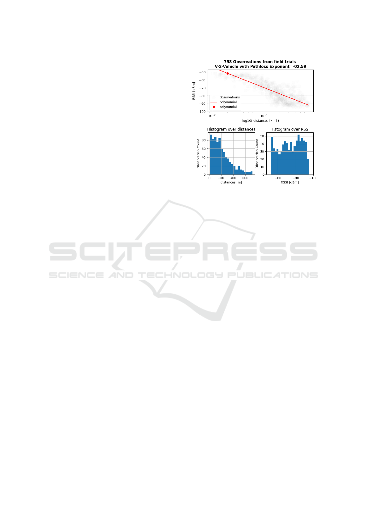
Figure 1: Measurements from test drives with RSSI vs

RSU-OBU distance (top) and the histograms over distances

and RSSI levels (below)).

The paper is organized as follows: The next sec-

tion introduces the theoretical background for pre-

diction of radio propagation and real-world measure-

ments. Section 2.2 summarizes the ﬁndings, includ-

ing a comparison between prediction and measured

values. The paper is concluded in the last section.

2 METHODOLOGY

In the current iteration of the proposed tool, a user

ﬁrst identiﬁes signalized intersections, which are to

be equipped with RSU. In a second step, informa-

tion of the desired coverage area (e.g., the registra-

tion points for public transport) have to be obtained.

Last, the user has to manually position the potential

RSU, considering constraints such as exiting posts,

ductwork, maximum cable length, etc. The tool then

uses a path-loss model as described below to predict

V2X radio propagation and checks if reception lev-

els are satisfactory for the given coverage area. If this

is not the case, the RSUs have to be either moved to

other positions or additional RSU have to be added.

2.1 Path-Loss Model and Link Budget

A simpliﬁed path-loss model according to (Gold-

smith, 2005) is used to estimate reception levels

caused by a RSU. This deliberately circumvents

the modeling of reﬂections, shadowing, and fast fad-

ing effects. Obstacles due to trafﬁc ﬂows are also

not considered and would require a statistical mod-

eling. Typically, data packets are transmitted with a

A Tool for V2X Infrastructure Placement

639

Figure 2: Measurement setup used for data gathering. On

the left is the RSU mounted on a mobile tripod, on the right

is the vehicle used for measurements. The V2X antenna is

visible on the top of the car.

robust and interference resistant modulation and cod-

ing scheme in accordance with the ITS-G5, so a V2X

message can be reliably received within cell bound-

aries. The penetration density of the radio channel

is not a limiting parameter due to the low trafﬁc vol-

ume and small message size. A major focus was set

to identify the Line-of-Sight (LOS) or Non-Line-of-

Sight (NLOS) radio conditions between the transmit-

ter and receiver geometry, the main source of obstruc-

tions being buildings. Therefore, the building loca-

tions were extracted from OpenStreetMap (OSM) as

described in detail in the next section.

The RSU transmits with the highest allowed

power of 23.0 dBm within the frequency band for

V2X of 5.9 GHz. Due to the possible antenna po-

sitions at the masts, we consider a feeder loss of

−2.5dB and an omnidirectional modeled transmit-

ting antenna with 2.0dBi gain. Geometric perspec-

tives are taken into account in the antenna pattern, the

distance between RSU and OBU, as well as the rel-

ative height of 5.0 m. Ultimately, distances greater

than 750.0 m are not further modeled, as these are

not typical in an urban environment. The RSUs and

OBUs used are from the Cohda Wireless (see Section

2.3 below), which have a minimum reception level of

−100.0dBm, so that this parameter is used as a fur-

ther termination criterion for the modeling.

The path-loss coefﬁcient was determined from

several measurement runs at various intersections and

RSU masts in Chemnitz. The power losses were

determined over the distance between the RSU and

OBU. The path-loss coefﬁcient results in the double-

logarithmic representation as the slope of a regression

line (see Fig. 1). During the measurement campaign,

multiple situations occurred in which other road users

Table 1: The list of parameters for the link budget.

Link Budget Parameter Value

Transmit Power 23.0dBm

Feeder Loss −2.5dB

Omnidirectional RSU antenna 2.0dBi

Isotropic OBU antenna 0.0dBi

Height between RSU and OBU 5.0m

Path-loss exponent 2.6

Reference distance 20.0m

Reference offset −74.1dB

Penalty term for NLOS condition −33.0dB

Maximal transmission radius 750.0m

Minimal OBU sensitivity −100.0dBm

crossed the direct line of sight and thus caused addi-

tional attenuation. In order not to weight such mea-

sured values and to remove the temporal bias by stop-

ping at certain positions, the measurements were di-

vided into segments of 10.0m and only the median

value of the upper 20% percentile of all Received Sig-

nal Strength Indicator (RSSI) was selected to avoid

that obstacles downgrade the estimates. This assump-

tion is regarded valid since a constant transmit power

without a power control operates at the RSU side.

Furthermore, positions with a distance closer than

10.0m respectively RSSIs> −50.0dBm are ignored.

Finally, a path-loss coefﬁcient of 2.6 dB per decade

was estimated and used to model the propagation en-

vironment. The table 1 summarizes all the included

parameters for the link budget.

2.2 Environmental Model via OSM

The decisive factor that inﬂuences the transmission /

reception conditions is the building environment and

the determination of the LOS and NLOS reception

conditions. The layouts of the buildings listed in

OSM were used for this purpose. The direct path

from RSU to OBU was sampled every 10.0 m and

their geocoordinates led to an Overpass-API query to

determine if the point was located within a building.

In the case of a building, the path was classiﬁed as

NLOS and the additional path-loss of −33.0dB was

used as the penalty term. The value of the penalty

term was not determined, only speciﬁed heuristically.

OSM was also used to extract reception points on the

roads used in the modeling.

VEHITS 2025 - 11th International Conference on Vehicle Technology and Intelligent Transport Systems

640

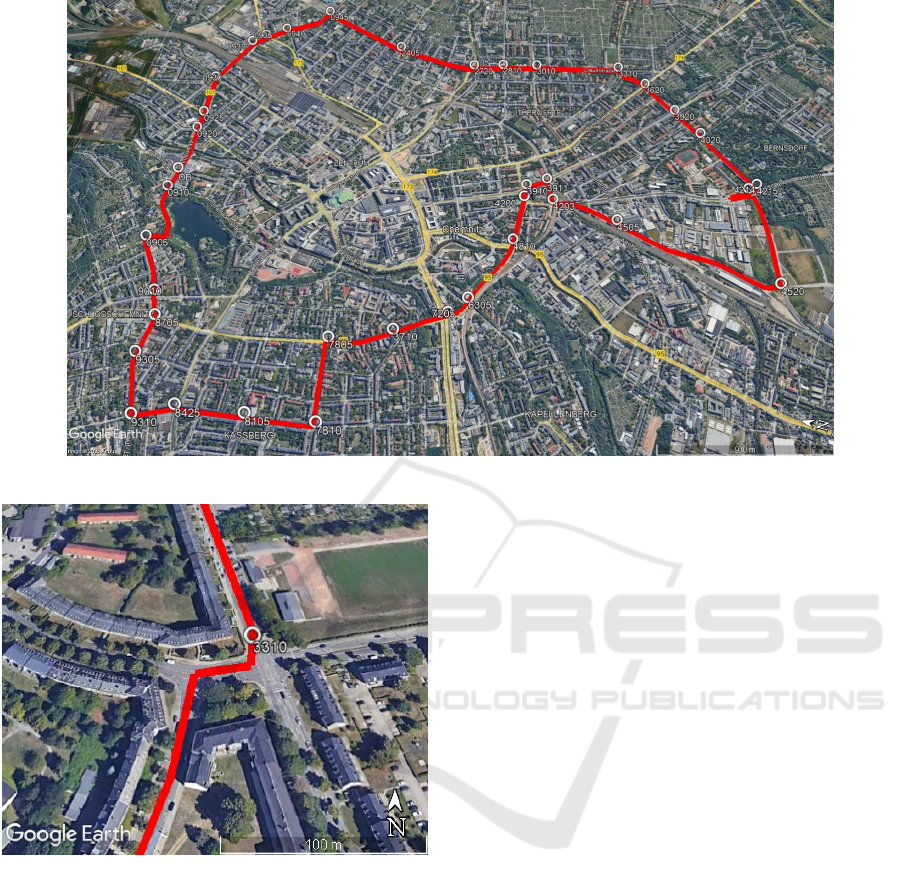
Figure 3: Route of the bus line 82 in Chemnitz, together with all (a total of 38) signalized intersections crossed by this line.

Figure 4: Example of one intersection, where manual mea-

surements were conducted.

2.3 On-site Measurements

The measurement system for real-life measurements

consists of an RSU mounted on a mobile post and an

OBU mounted in a test vehicle. For both units, a Co-

hda MK5 was employed, which used a custom com-

munication stack each (C4CART (Jacob et al., 2020)).

The mobile RSU was modiﬁed for battery operation.

Additionally, both OBU and RSU were equipped with

cellular communication units to facilitate connection

to a back-end server to allow real-time transmission of

measurement data. In case of loss of mobile connec-

tivity, measurement data can also be retrieved from

recorded .pcap ﬁles.

As we are mainly interested in deploying TSP, a

rather high vehicle (a Mercedes Vito) was used for the

measurements, which is higher than a typical passen-

ger vehicle. The complete measurement setup can be

seen in Fig. 2.

For localization, the internal Global Navigation

Satellite System (GNSS) modules of the respective

units were used. These offer an accuracy of 2.5 m

Circular Error Probable (CEP). For the measure-

ments, the CAM were used, which were send ac-

cording to the standard (ETSI EN 302 637-2 V1.4.1

(2019-04), 2019). This means that the RSU sends

messages with 1Hz, while the vehicle sends messages

with 1Hz − 10 Hz, depending on the dynamic state of

the vehicle.

2.4 Limitations of the Model

Task of this evaluation is not an exact reproduction

of the physical propagation behavior, but to get a

solid idea of the placement of the RSUs. In partic-

ular, the cell borders need further visual inspections,

since local obstacles might not be covered even in

high-resolution maps. Furthermore, a constant height

difference between sender and receiver is assumed

(comp. Table 1), which is not always true due to

the local topography. In addition, the low accuracy

of 2.5 m CEP in the GNSS measurements potentially

causes large differences between the reported and ac-

tual positions. Under some circumstances this leads

to a wrong assignment of a NLOS connection, when

comparing simulation with real world measurements.

A Tool for V2X Infrastructure Placement

641

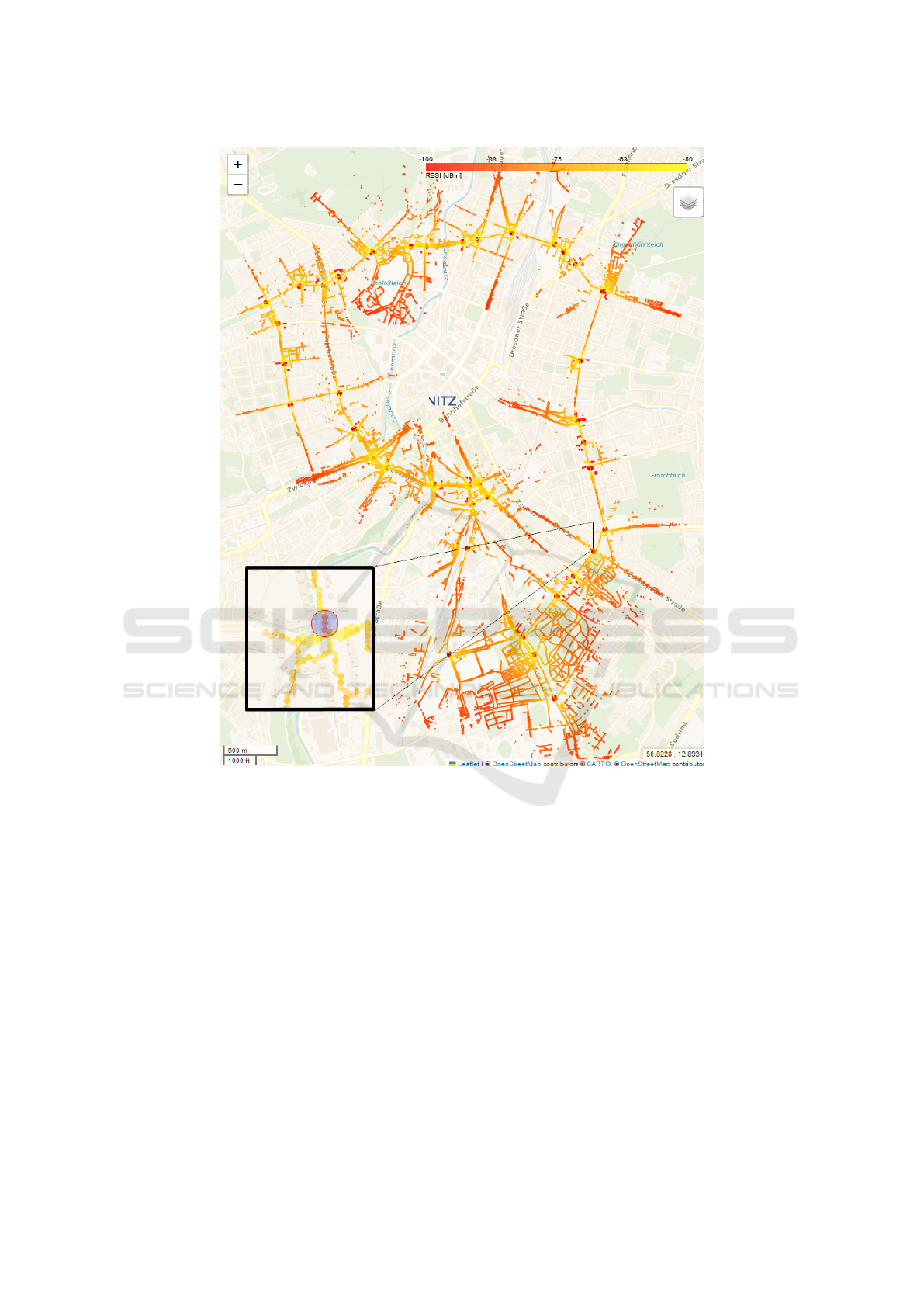
Figure 5: The proposed tool outputs the result as web page. Depicted are the prediction of RSSI levels at all signalized

intersections connected to bus line 82 (compare Fig. 3). Enlarged, in the lower left corner, are the results for the intersection

shown in Fig. 4. The red circle marks the position of the RSU. Overall, a good connectivity is predicted across the whole

route, when using the current positions of RSU.

3 EVALUATION AND

DISCUSSION

The proposed tool was used to plan the installation

of RSU along the bus line 82 in the city of Chem-

nitz, Germany. This bus line crosses a total of 40 sig-

nalized intersections and crossings, where 38 trafﬁc

lights are equipped for prioritization (see Fig. 3). For

all intersection RSU placement was evaluated using

the tool using an estimated path-loss exponent. Of

these intersections, 15 were considered critical, that

is, the predicted range seemed insufﬁcient to realize

the intended use case, that is, the preregistration loca-

tion was not covered or had only minimal radio cover-

age. One of these intersections is shown in Fig. 4. At

this speciﬁc intersection, the bus line route does not

follow the main road but instead takes a turn. As a re-

sult, one could expect a signiﬁcant blockage of V2X

communication due to buildings. Manual measure-

ments were planned at these intersections to assess

whether the placement of secondary RSU would be

required. Due to road construction works, measure-

ments could only be taken for 11 of the identiﬁed in-

tersections. Consequently, these measurements were

used to evaluate the accuracy of the predictions.

For evaluation, the measurement area was divided

into hexagons. For a given position of the RSU, RSSI

VEHITS 2025 - 11th International Conference on Vehicle Technology and Intelligent Transport Systems

642

1 1

2 7

6 0

7 6

9 2

1 2 4

1 1 3

1 1 1

9 6

5 5

3 0

1 8

1 0

0 0 0 0

- 1 0 0 1 0 2 0 3 0 4 0

5 0

1 0 0

1 5 0

C o u n t

m e a s u r e d

- P

p r e d

[ d B m ]

Figure 6: Comparison of real world measurements vs. the

predictions. The mean difference is 0.99 dBm with a stan-

dard deviation of 7.35 dbm. Values on the right result from

a too pessimistic modeling.

levels were predicted (see Fig. 5 for an example).

These were compared against the RSSI measured

during the test drive. In case there was more than

one measurement per hexagon, the 80% percentile of

all measurements was used. This was done to ex-

clude certain cases of NLOS, e.g., if communication

was blocked by another vehicle. For evaluation, 841

predicted values were compared with measurements,

where the measured values were retrieved from all

intersections included in the measurement campaign.

The result of this comparison can be seen in Fig. 6.

The difference between measured and predicted val-

ues usually lies between −15dBm − 20 dBm, with

some outliers greater than 25 dBm. These outliers

could be traced to an erroneously assigned NLOS

connection. This is due to the inaccuracy in GNSS,

i.e., the reported position resulted in NLOS connec-

tion, but the real position had LOS.

Generally, modeling differences larger than 0 dBm

do not cause problems, as long as all registration

points are still covered (for the case of TSP), as

this means that the actual connection was even better

than predicted. Values smaller than 0 dBm are more

concerning. Detailed investigations have shown that

these values appear mainly near the submitting sta-

tion, which means that some propagation properties

of the radios are not fully considered by the path-loss

model. As reception levels near the radio are typically

very high, this does not cause an issue for the overall

tool.

Although previous research (Eltahir, 2007) has

shown that the choice of the radio propagation model

has a signiﬁcant impact on the results of the simu-

lations, our results actually validate the choice of a

simple path-loss model with a penalty term for NLOS

connections, at least if used for V2X infrastructure

planning. Compared to the ray-launching method

proposed by Granda et al. (Granda et al., 2017),

a similar mean error was achieved (0.99 dBm here

vs. 1.75 dBm). In contrast, their method achieves

a much lower standard deviation (2.54 dBm) ver-

sus 7.35 dBm. Although the results obtained us-

ing the ray-launching method are more accurate, ray-

launching requires ray-tracing software and hardware,

which are rather expensive to obtain and to oper-

ate, whereas the proposed algorithm runs on an of-

ﬁce notebook. Given that V2X planning is mainly

contracted by public communities, the offset in costs

could justify the use of a less accurate model, espe-

cially if the results are still good enough for the de-

sired task.

4 CONCLUSIONS & OUTLOOK

Taking real-world measurements for 11 of the 38 sig-

nalized intersections required two people and a day of

work. Measurement of all intersections would have

taken nearly a week. In comparison, generating the

predictions took less than twenty minutes on an of-

ﬁce notebook, most of this computation time. In gen-

eral, the proposed approach leads to a signiﬁcant de-

crease in planning RSU placement. Furthermore, it

was shown that the model was able to sufﬁciently pre-

dict real-world radio propagation. Although the com-

parison was performed using IEEE 802.11p, it can be

equally used for C-V2X as the physical propagation

and radio frequencies are the same for both technolo-

gies.

However, there are some limitations of the cur-

rent approach. It works best when the local path-

loss exponent can be accurately estimated, which still

relies on real-world measurements. This is neces-

sary, as this exponent can vary wildly given the local

circumstances, for example, (Goldsmith, 2005) cites

measured path-loss exponents between 2.7 − 6.5. On

the other hand, already existing RSU could help with

this part by comparing reception levels with the posi-

tion reported in the CAM by connected vehicles al-

ready on the road today. Furthermore, currently a

constant difference between the height of RSU and

OBU are assumed. Although the model could also

handle varying height differences, this would com-

plicate the computations, e.g., buildings would need

to be checked for NLOS connections, but also the

ground, especially in hilly regions.

The current approach relies on OSM data. Since

this is an open-source effort, the quality of the data

differs. For some regions in Germany, for example,

Saxony, there exists a digital height model with 25 cm

A Tool for V2X Infrastructure Placement

643

resolution, which is captured from ﬂight data. In ad-

dition to the higher accuracy, these data also contain

information on larger plants and their spread.

In the future, machine learning is planned to

be used for propagation prediction. Given enough

training and meta-data, it is assumed that some

kind of neural net can estimate the path-loss expo-

nent/propagation sufﬁciently. This would eliminate

the need to determine a path-loss exponent. In addi-

tion, in the current iteration, the position of the RSU

is still determined by hand. In a future iteration, this

position could also be computed using optimization

algorithms, which could consider constraints like the

distance to the trafﬁc light controller (depending on

transmission technology, for example not longer than

100 meters for Power-over-Ethernet (PoE)) and phys-

ical restrictions on placement.

ACKNOWLEDGEMENTS

This research is ﬁnancially supported by the project

ITS4Culture. Parts of the paper were translated from

German to English using a custom version of Chat-

GPT (FhGenie). Writefull AI was used to increase

the readability of the manuscript.

REFERENCES

Astudillo Le

on, J. P., Busson, A., de la Cruz Llopis,

L. J., Begin, T., and Boukerche, A. (2024). Strate-

gic deployment of rsus in urban settings: Optimiz-

ing ieee 802.11p infrastructure. Ad Hoc Networks,

163:103585.

Eltahir, I. K. (2007). The impact of different radio prop-

agation models for mobile ad hoc networks (manet)

in urban area environment. In The 2nd International

Conference on Wireless Broadband and Ultra Wide-

band Communications (AusWireless 2007), pages 30–

30.

ETSI EN 302 637-2 V1.4.1 (2019-04) (2019). ETSI EN

302 637-2 V1.4.1 (2019-04) Intelligent Transport Sys-

tems (ITS); Vehicular Communications; Basic Set of

Applications; Part 2: Speciﬁcation of Cooperative

Awareness Basic Service. Standard, ETSI.

Gay, M., Grimm, J., Otto, T., Partzsch, I., Gersdorf,

D., Gierisch, F., L

owe, S., and Sch

utze, M. (2022).

Nutzung der c2x-basierten

Ov-priorisierung an signal-

isierten knotenpunkten. Technical report.

Goldsmith, A. (2005). Wireless communications. Cam-

bridge university press.

Granda, F., Azpilicueta, L., Vargas-Rosales, C., Lopez-

Iturri, P., Aguirre, E., Astrain, J. J., Villandangos,

J., and Falcone, F. (2017). Spatial characteriza-

tion of radio propagation channel in urban vehicle-to-

infrastructure environments to support wsns deploy-

ment. Sensors, 17(6).

Jacob, R., Gay, M., Dod, M., Lorenz, S., Jungmann,

A., Franke, L., Philipp, M., Kloeppel-Gersdorf, M.,

Haberjahn, M., Gruschka, E., and Fettweis, G. (2020).

Ivs-kom: A reference platform for heterogeneous its

communications. In 2020 IEEE 92nd Vehicular Tech-

nology Conference (VTC2020-Fall), pages 1–7.

Otto, T., Partzsch, I., Holfeld, J., Kl

oppel-Gersdorf, M., and

Ivanitzki, V. (2023). Designing a c-its communication

infrastructure for trafﬁc signal priority of public trans-

port. Applied Sciences, 13(13).

Schemel, H. et al. (1990). Technische Anforderun-

gen an rechnergesteuerte Betriebsleitsysteme -

Ubertragungsverfahren Datenfunk; Erg

anzung 2

“Datensatz f

ur Meldesysteme”. Technical report.

Young, W. F., Remley, K. A., Holloway, C. L., Koepke, G.,

Camell, D., Ladbury, J., and Dunlap, C. (2014). Ra-

diowave propagation in urban environments with ap-

plication to public-safety communications. IEEE An-

tennas and Propagation Magazine, 56(4):88–107.

VEHITS 2025 - 11th International Conference on Vehicle Technology and Intelligent Transport Systems

644