Assessment of Fine-Tuned Canopy Height Maps from Satellite Imagery:

A Case Study in the Czech Republic

Leonidas Alagialoglou

1 a

, Ioannis Manakos

2 b

, Olga Brovkina

3 c

, Jan Novotn

3 d

and

Anastasios Delopoulos

1 e

Multimedia Understanding Group, Aristotle University of Thessaloniki, Greece

Information Technologies Institute, Centre for Research and Technology Hellas, Thessaloniki, Greece

Department of Remote Sensing, Global Change Research Institute of the Czech Academy of Sciences, CzechGlobe,

Brno, Czech Republic

Keywords:

Canopy Height Estimation, Deep Learning, Fine-Tuning, Forest, Sentinel-2, Data-Centric AI, Uncertainty

Estimation, Tree Species, Airborne Laser Scanning.

Abstract:

This study evaluates the performance of a lightweight convolutional Long Short-Term Memory (ConvLSTM)-

based deep learning model for estimating canopy height across three test areas in the Czech Republic using

Sentinel-2 time series data. The model, initially trained on forest data from Germany and Switzerland, in-

corporate uncertainty quantiﬁcation techniques and was ﬁne-tuned and evaluated using dense airborne laser

scanning (ALS) data collected between 2022 and 2024. Results show that ﬁne-tuning reduced mean absolute

error (MAE) from 4.26 m to 2.74 m in the primary test area, with similar improvements across other regions.

Species-speciﬁc uncertainties were also analyzed, highlighting performance variations between deciduous and

coniferous forests.

1 INTRODUCTION

Accurate estimation of forest canopy height is cru-

cial for understanding forest structure, carbon storage

potential, and biodiversity (Zhang et al., 2016; Mao

et al., 2019; Lang et al., 2023). Traditionally, high-

resolution airborne laser scanning (ALS) has been

the benchmark for obtaining accurate canopy height

data (Brovkina et al., 2017; Douss and Farah, 2022;

Fischer et al., 2024). However, ALS is resource-

intensive and limited in spatial and temporal cover-

age. The alternative approaches are developing that

make use of readily available satellite data (Potapov

et al., 2021; Lang et al., 2023; Tolan et al., 2024).

Recent advancements in deep learning models have

enabled indirect estimation of canopy height using

satellite imagery, particularly time-series data from

Sentinel-2. Although Sentinel-2 does not provide

height information directly, its multispectral and tem-

https://orcid.org/0000-0002-8361-0589

https://orcid.org/0000-0001-6833-294X

https://orcid.org/0000-0001-5860-2184

https://orcid.org/0009-0004-1017-9160

https://orcid.org/0000-0001-8220-8486

poral characteristics allow for canopy structure infer-

ence when combined with appropriate machine learn-

ing models. Nevertheless, challenges remain in adapt-

ing models trained on one geographic region to new

areas with different ecological and distributional char-

acteristics. Fine-tuning models with local ALS data

is a promising strategy for improving transferability

and accuracy. In this study, we leverage dense ALS-

derived canopy height maps as ground-truth data to

train and validate a deep learning model that predicts

canopy height from Sentinel-2 time-series imagery.

This study contributes to the developing deep-

learning approaches for canopy height estimation

from satellite imagery. It evaluates the performance

of Convolutional Long Short-Term Memory (ConvL-

STM) based models on three Czech test areas. The

models process 40 or more Sentinel-2 (S-2) time-

frames spanning an entire year and provide uncer-

tainty estimates using deep ensembles with isotonic

regression calibration (Alagialoglou et al., 2022).

Ground-truth data for training were sourced from the

Bohemian Forest and Switzerland, and ﬁne-tuning

was performed on site-speciﬁc data.

We aim to provide insights into the reliability of

Sentinel-2 derived canopy height maps for local ap-

236

Alagialoglou, L., Manakos, I., Brovkina, O., Novotný, J. and Delopoulos, A.

Assessment of Fine-Tuned Canopy Height Maps from Satellite Imagery: A Case Study in the Czech Republic.

DOI: 10.5220/0013475200003935

Paper published under CC license (CC BY-NC-ND 4.0)

In Proceedings of the 11th International Conference on Geographical Information Systems Theory, Applications and Management (GISTAM 2025), pages 236-243

ISBN: 978-989-758-741-2; ISSN: 2184-500X

plications. The objectives of this study are to:

• Assess the performance of ﬁne-tuned ConvLSTM

models for estimating canopy height in Czech

forests.

• Compare the accuracy of ﬁne-tuned models with

their pretrained counterparts.

• Quantify species-speciﬁc uncertainties for decid-

uous and coniferous trees.

2 MATERIALS & METHODS

2.1 Study Areas

The three test areas are located in the Moravian region

of the Czech Republic spanning 3.5 km

, 11 km

, and

3 km

, as shown in ﬁgure 1. The three study areas

were selected to represent different forest composi-

tions and ecological conditions, allowing us to assess

model performance across diverse environments. The

forests in Test Areas 1 and 2 are predominantly decid-

uous, with a small mixture of spruce and pine. Test

Area 3 consists mostly of coniferous forest (Fig. 2).

2.2 ALS and Sentinel-2 Data

Airborne laser scanning (ALS) data were acquired us-

ing the Riegl LMS Q780 airborne full-waveform laser

scanner, which was mounted on the Flying Labora-

tory of Imaging Systems (FLIS) operated by Czech-

Globe (https://olc.czechglobe.cz/en/home-en/). ALS

data were collected during the years 2023, 2022, and

2024, for the test areas 1, 2, 3 respectively. The ac-

quisition details, including point cloud density and

Sentinel-2 availability, are summarized in Table 1.

Fine-tuning of the model was conducted on a 1.4 km

subset of Test Area 2, marked in pink color on ﬁg-

ure 1. The acquisition details are summarized in Ta-

ble 1, with some additional information of the avail-

able Sentinel-2 imagery of the speciﬁc study areas.

Despite variations in the point cloud density of the

acquired ALS data across the test areas, they are con-

sidered dense ground truth maps due to their signif-

icantly higher density compared to the interpolated

resolution of the smallest Sentinel-2 ground sampling

distance (10 m).

The ALS data processing workﬂow included tra-

jectory calculation, georeferencing, relative orienta-

tion of individual ﬂight lines, and export. These

steps were conducted using a combination of software

tools provided by the scanner manufacturer (POSPac

8.7, RiPROCESS 1.9.2, RiUNITE, GeoSysManager

2.2.4) and the LAStools software suite. The result-

ing laser point clouds were exported and further pro-

cessed into digital surface models (DSM).

The processed ALS data provide highly accurate

canopy height information and serve as dense ground

truth references for model training and evaluation.

The derived DSM spatial resolution is 0.5 m, ensuring

detailed spatial representation of the forest canopy.

A sequence of Sentinel-2 (S-2) Level-1C prod-

ucts, representing top-of-atmosphere reﬂectance, of

the study areas is downloaded for the years of each

ALS data acquisition, from the Copernicus Datas-

pace Ecosystem. The number of available products

for each area is given in table 1. Sentinel-2 imagery

was collected across all seasons without cloud ﬁlter-

ing, ensuring coverage throughout the year. All model

inputs and outputs were resampled to a 10 m spatial

resolution to match Sentinel-2’s highest available res-

olution.

Tree species classiﬁcations were derived from the

Forest Management Institute (FMI) dataset for 2022

2.3 Model Architecture

The ConvLSTM models combine convolutional lay-

ers with long short-term memory (LSTM) networks

to effectively process spatial and temporal data. The

models were initially trained on Sentinel-2 imagery,

using 40 timeframes per year, and calibrated with iso-

tonic regression to produce uncertainty maps. Train-

ing data included regions in the Bavarian Forest and

forested areas in the whole area of Switzerland. Fur-

ther details on the training dataset and neural network

architecture are available in our previous study (Ala-

gialoglou et al., 2022).

The ensemble of models is ﬁne-tuned on a sub-

set of Test Area 2, speciﬁcally for the year 2022, as

depicted in Figure 1. Fine-tuning employs the Gaus-

sian Negative Log Likelihood loss function, as rec-

ommended in our earlier work (Alagialoglou et al.,

2022). Optimization is performed using the AdamW

optimizer with a weight decay regularization coefﬁ-

cient of 1 × 10

−3

and a learning rate of 1× 10

−4

, over

100 epochs.

During inference, the model processes 40 uni-

formly distributed timeframes for a given year with-

out applying any cloud ﬁltering. In practice, more

timeframes are utilized by ensembling the results of

150 runs, with each run using a different set of 40 in-

puts.

https://geoportal.uhul.cz/mapy/MapyDpz.html

Assessment of Fine-Tuned Canopy Height Maps from Satellite Imagery: A Case Study in the Czech Republic

237

Figure 1: Overview of three test areas in the Czech Republic, covering 3.6 km

, 10 km

, and 3 km

, respectively. ALS

reference data were collected in 2023, 2022, and 2024. Fine-tuning was performed on a 1.4 km

subset of Test Area 2,

highlighted in pink. The central coordinates of each test area are: Test Area 1 – (16.833260, 49.004164), Test Area 2 –

(16.945512, 48.681688), and Test Area 3 – (16.180660, 49.313461).

Table 1: Overview of parameters for the three study areas, including ALS data acquisition and Sentinel-2 acquisitions.

⋆

The ﬁne-tuning area is a small sub-region within study area 2, as shown in Figure 1.

Study Area Acquisition Date Area [km

]

Cloud Point Density

[points/m

]

Total Sentinel-2 Scenes

1 28.05.2023 3.6 10 145

⋆

13.07.2022 10.0 8 144

3 30.04.2024 3.0 10 65

Figure 2: Species distribution in the test areas 1-3 and the

ﬁne-tune area.

2.4 Experimental Design

Two experimental setups were evaluated:

1. Pretrained Models: These models were applied

without ﬁne-tuning, resulting in higher estimation

errors.

2. Fine-Tuned Models with Dense Ground-Truth:

These models were ﬁne-tuned using dense Li-

DAR data covering approximately 1.4 km

. The

ﬁne-tuning area corresponds to a subregion of

Test Area 2, as shown in Figure 1. In terms

of species representation, this sub-region follows

similar species distribution with the total Test

Area 2. However, it is very different to the species

distribution of Test Area 3. With this choice we

aim to examine the ﬁne-tuned model performance

on test areas with both similar as well as different

forest type characteristics.

Species-speciﬁc uncertainties were computed us-

ing tree species maps provided by the Forest Man-

agement Institute (FMI) for the reference year 2022.

Exploratory statistics of species distributions across

the three study areas are illustrated in Figure 2. The

species map, originally a vector layer, was rasterized

to match the Sentinel-2 resolution with a ground sam-

pling distance of 10 m, using nearest-neighbor inter-

polation.

The performance of the canopy height models

was evaluated using three quantitative metrics: Mean

Absolute Error (MAE), Root Mean Square Error

(RMSE), and the Coefﬁcient of Determination (R

• MAE: average absolute difference between the

predicted and observed values. MAE provides

an intuitive measure of overall error, expressed in

meters.

• RMSE: square root of the average squared differ-

ences between the predicted and observed values.

RMSE penalizes larger errors more heavily, mak-

ing it sensitive to outliers, and is also expressed in

meters.

GISTAM 2025 - 11th International Conference on Geographical Information Systems Theory, Applications and Management

238

• R

: Represents the proportion of variance in the

observed data that is explained by the model.

An R

value close to 1 indicates strong agree-

ment between the predicted and observed values,

while values near 0 suggest poor predictive per-

formance.

3 RESULTS

Figure 3 presents canopy height estimation results for

the three test areas, including absolute error maps and

quantitative metrics such as mean absolute error, root

mean square error and R

. These ﬁgures provide a vi-

sual comparison of the errors associated with the pre-

trained and ﬁne-tuned models across the test areas.

Speciﬁcally, for Test Area 1, the ﬁne-tuned model

achieved a MAE of 1.09m, RMSE of 2.09m, and R

of 0.88, compared to the pretrained model’s MAE of

1.27m, RMSE of 2.24m, and R

of 0.87. In Test Area

2, the ﬁne-tuned model achieved a MAE of 2.69m,

RMSE of 3.63m, and R

of 0.83, compared to the pre-

trained model’s MAE of 4.45m, RMSE of 5.52m, and

of 0.62. Similarly, in Test Area 3, the ﬁne-tuned

model achieved a MAE of 1.48m, RMSE of 2.51m,

and R

of 0.66, compared to the pretrained model’s

MAE of 2.04m, RMSE of 3.18m, and R

of 0.46. The

visual comparison further underscores the improve-

ment, with reduced absolute error maps for ﬁne-tuned

models.

Based on the quantitative results and visual anal-

ysis shown in Figure 3, the ﬁne-tuned model is over-

all accurate for all three test areas in different years,

comparing to the state-of-the-art (Alagialoglou et al.,

2022; Lang et al., 2023; Tolan et al., 2024), with as

little as 1.4km

ﬁne-tuning ground-truth area. Fur-

thermore, the ﬁne-tune model consistently demon-

strated superior performance compared to the pre-

trained model across all test areas and all vegeta-

tion types, as evidenced by all three metrics: MAE,

RMSE, and R

. This consistent trend across all test

areas validates the efﬁcacy of the ﬁne-tuning process

in improving model performance.

Similar conclusions are demonstrated in tables 3

and 4. Test Area 2 showed the most signiﬁcant reduc-

tions in the overall MAE and RMSE for the ﬁne-tuned

models, particularly for deciduous species. This can

be attributed to two factors:

1. The ﬁne-tuning area is a subregion of Test Area

2 for the same year, allowing the models to better

adapt to the speciﬁc distribution characteristics of

the area and time.

2. Test Areas 1 and 3 contain large regions domi-

nated by the ”Plantation/Other” class, which gen-

erally exhibits lower canopy height values and,

consequently, smaller errors and lower margin for

improvement.

Detailed quantitative results for each species

across the three test areas are summarized in Tables

3 and 4. These tables demonstrate that the ﬁne-tuned

model consistently outperforms the pretrained model

across all test areas and species, with signiﬁcant re-

ductions in both MAE and RMSE. The results show

metrics for six species categories, as well as overall

metrics for each test area. Species categories include

Spruce, Pine, Oak, Other Deciduous, Other Conifer-

ous, and Plantation/Other. The metrics are provided

for both pretrained and ﬁne-tuned models to enable

direct comparison.

The Oak class, representing approximately 50%

of the ﬁne-tuning dataset, dominates the model’s

learning and exhibits the most consistent accuracy im-

provements across all test areas with sufﬁcient land

cover percentages. For instance, in Test Area 2, the

ﬁne-tuned model achieves a MAE of 2.89 m, com-

pared to 5.13 m for the pretrained model. Simi-

larly, in Test Area 1, which corresponds to a different

year, the ﬁne-tuned model yields a MAE of 3.23 m,

outperforming the pretrained model’s MAE of 4.51

m. This trend is also evident in Figure 4. In Test

Area 2, the MAE difference between the pretrained

and ﬁne-tuned models for shorter oak trees (1–4 me-

ters) exceeds 1.5 times the actual canopy height. In

contrast, the ”Other deciduous” and ”Plantation &

Other” classes show MAE improvements closer to 1

times the actual canopy height. Additionally, the ﬁne-

tuned model demonstrates consistent accuracy im-

provements for the class Oak across all canopy height

bins, as seen in the left panel of Figure 4. This im-

provement aligns with the class proportions in the

ﬁne-tuning dataset, where Oak dominates (50%), fol-

lowed by ”Plantation & Other” and ”Other Decidu-

ous”.

Test Area 2, at 10 km

, is signiﬁcantly larger than

Test Area 1 (3.6 km

) and Test Area 3 (3 km

). The

species distribution in Test Areas 1 and 2 primarily

incudes deciduous trees, while Test Area 3 is mostly

coniferous, excluding the ”Plantation/Other” class.

For this reason, the analysis focuses on the dominant

forest classes, avoiding those with small sample sizes.

It is noted that the performance of classes with few

pixels, such as the oak in Test Area 3 or the spruce

and pine in Test Area 1, should not be taken into con-

sideration. Due to the limited number of pixels avail-

able for these classes, results are likely affected by

label noise in the species classiﬁcation map. How-

ever, although oak is generally absent in Test Area 3,

similarly to spruce and pine in Test Area 1, the results

Assessment of Fine-Tuned Canopy Height Maps from Satellite Imagery: A Case Study in the Czech Republic

239

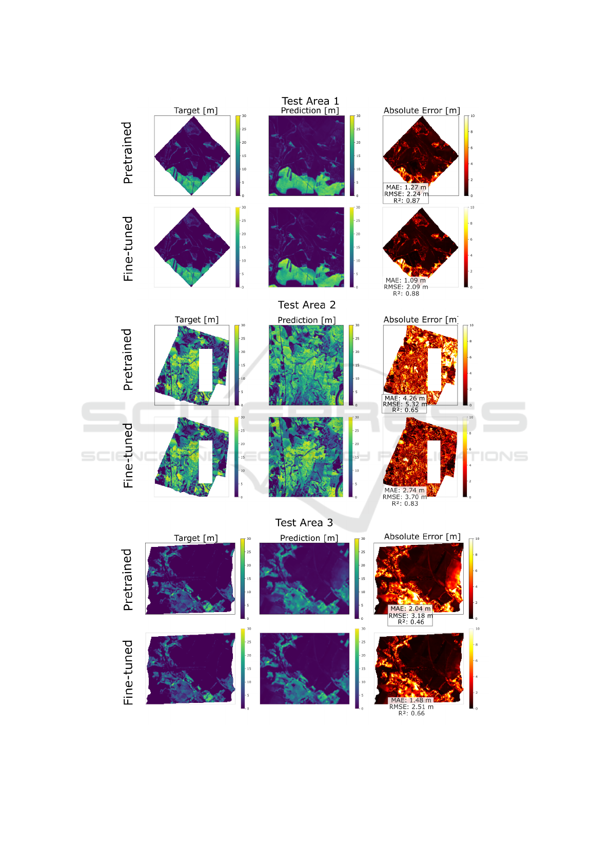
Figure 3: Results for the tree test areas: pretrained and ﬁne-tuned models.

GISTAM 2025 - 11th International Conference on Geographical Information Systems Theory, Applications and Management

240

Table 2: Mean and Standard Deviation (std) for ALS measurements and predictions (Pretrained and Fine-tuned), along with

number of pixels (n), by Class and Test Area.

Class Test Area 1 Test Area 2 Test Area 3

ALS

mean (std)

Pretrained

mean (std)

Fine-tuned

mean (std)

ALS

mean (std)

Pretrained

mean (std)

Fine-tuned

mean (std)

ALS

mean (std)

Pretrained

mean (std)

Fine-tuned

mean (std)

Spruce 5.73 (5.27) 5.26 (4.12) 5.37 (4.60) 83 5.16 (5.22) 6.95 (4.08) 6.28 (4.66) 485 6.28 (4.52) 9.52 (5.08) 8.39 (5.12) 3084

Pine 11.48 (3.63) 9.60 (3.54) 9.77 (3.59) 56 11.53 (3.56) 13.54 (3.28) 12.25 (3.16) 1514 11.24 (6.10) 13.69 (4.21) 13.85 (5.17) 1567

Oak 16.18 (4.61) 20.59 (3.36) 18.17 (3.36) 1541 15.02 (7.18) 18.64 (4.58) 15.80 (6.03) 32837 6.26 (2.90) 15.80 (3.03) 12.09 (2.80) 284

Other Deciduous 14.96 (6.00) 17.50 (6.43) 16.47 (6.40) 4193 16.65 (8.09) 16.14 (5.71) 17.29 (7.15) 39060 6.58 (4.60) 11.21 (4.89) 10.08 (5.06) 1414

Other Coniferous 13.03 (5.88) 15.49 (7.03) 14.61 (6.79) 582 11.30 (7.74) 11.66 (6.22) 11.42 (6.89) 4115 6.72 (4.56) 10.36 (4.66) 9.63 (5.06) 2215

Plantation/Other 0.68 (1.54) 0.93 (1.22) 0.75 (1.29) 29637 1.98 (3.61) 4.71 (4.53) 2.93 (3.86) 20711 0.39 (1.33) 1.49 (2.18) 1.03 (1.92) 21913

Overall 3.23 (6.15) 4.59 (7.70) 4.07 (7.12) 36092 12.67 (9.00) 14.71 (7.51) 13.36 (8.33) 98722 2.35 (4.31) 4.03 (5.25) 3.45 (5.12) 30477

Table 3: MAE and number of pixels (n) for Pretrained and Fine-tuned Models by Class and Test Area.

Class Test Area 1 Test Area 2 Test Area 3

Pretrained

MAE [m]

Fine-tuned

MAE [m]

Pretrained

MAE [m]

Fine-tuned

MAE [m]

Pretrained

MAE [m]

Fine-tuned

MAE [m]

Spruce 1.74 1.60 83 3.33 2.73 485 3.80 2.76 3084

Pine 2.35 2.39 56 2.91 2.62 1514 3.96 3.67 1567

Oak 4.51 3.23 1541 5.13 2.89 32837 9.61 5.90 284

Other Deciduous 3.51 3.44 4193 4.23 3.23 39060 4.93 3.91 1414

Other Coniferous 3.54 3.32 582 3.73 3.23 4115 4.23 3.55 2215

Plantation/Other 0.74 0.60 29637 3.17 1.49 20711 1.15 0.72 21913

Overall 1.27 1.09 36092 4.26 2.74 98722 2.04 1.48 30477

Table 4: RMSE and number of pixels (n) for Pretrained and Fine-tuned Models by Class and Test Area.

Class Test Area 1 Test Area 2 Test Area 3

Pretrained

RMSE [m]

Fine-tuned

RMSE [m]

Pretrained

RMSE [m]

Fine-tuned

RMSE [m]

Pretrained

RMSE [m]

Fine-tuned

RMSE [m]

Spruce 2.32 2.06 83 3.97 3.52 485 4.51 3.47 3084

Pine 2.58 2.62 56 3.81 3.23 1514 4.74 4.40 1567

Oak 5.57 4.51 1541 6.14 3.78 32837 10.31 6.42 284

Other Deciduous 4.50 4.44 4193 5.22 4.16 39060 5.83 4.75 1414

Other Coniferous 4.71 4.45 582 4.70 4.22 4115 5.12 4.40 2215

Plantation/Other 1.09 1.02 29637 4.28 2.35 20711 1.83 1.31 21913

Overall 2.24 2.09 36092 5.32 3.70 98722 3.18 2.51 30477

Figure 4: Left: Difference between the ﬁne-tuned model’s MAE and the pretrained model’s MAE, normalized by ground-truth

canopy height, for each tree species class across bins of ground-truth canopy height. Right: MAE for each tree species class

across bins of ground-truth canopy height. Tree species with less than 200 pixels per height bin are not plotted for clarity.

in tables 2, 3 and 4 are included for completeness.

The left part of Figure 4 presents the difference

in MAE between the ﬁne-tuned model and the pre-

trained model, normalized by ground-truth canopy

height, for each tree species class across bins of

ground-truth canopy height. The higher the normal-

ized ∆MAE, the more signiﬁcant the improvement

achieved by ﬁne-tuning with this speciﬁc dataset. On

the right side of the ﬁgure, the MAE for each species

class is displayed across the same bins. In both ﬁg-

ures, classes with less than 200 pixels per height bin

are not plotted for clarity.

Assessment of Fine-Tuned Canopy Height Maps from Satellite Imagery: A Case Study in the Czech Republic

241

Using the normalized MAE difference shown in

Figure 4, we observe that in Test Area 2, the Oak class

exhibits the most signiﬁcant improvement, followed

by the ”Plantation & Other” and ”Other deciduous”

classes, which improve similarly. The ”Other conif-

erous” class shows the least improvement. This order

corresponds to the class proportions in the ﬁne-tuning

dataset: Oak accounts for 50%, ”Plantation & Other”

for 31%, ”Other deciduous” for 14%, and ”Other

coniferous” for only 4%. Although these results align

with expectations based on the dataset composition,

one should be cautious, since tree species representa-

tion in the ﬁne-tuning dataset is an important factor

but not the sole determinant of model performance.

4 CONCLUDING REMARKS

The ﬁne-tuned model demonstrates high accuracy

across all three test areas in different years, outper-

forming state-of-the-art approaches with as little as

1.4 km² of ﬁne-tuning ground-truth data. It consis-

tently surpasses the pretrained model in all test areas

and vegetation types, with particularly notable accu-

racy improvements in the Oak class across all canopy

height bins, likely due to its dominance in the ﬁne-

tuning dataset. Moreover, species showing the most

signiﬁcant improvements correspond to their propor-

tions in the ﬁne-tuning data, reinforcing expectations

based on dataset composition. However, caution is

needed, as species representation is a crucial factor

but not the sole determinant of model performance.

This study underscores the importance of evaluating

the distribution characteristics of ﬁne-tuning datasets

to ensure reliable and localized conclusions.

Recent studies showed that the accuracy of CHMs

derived from satellite data varies between deciduous

and coniferous forests due to differences in canopy

structure, spectral reﬂectance, and other biophysical

properties. For instance, (Alvites et al., 2024) re-

ported that CHM accuracy differed signiﬁcantly be-

tween forest types, with the highest RMSE as a per-

centage of the mean observed data reaching 17.79%

in broadleaf forests and 26.58% in coniferous forests,

indicating higher errors in canopy height estimation

for coniferous forests. Our research does not offer

such insights however offers the perspective of the

correlation between the model’s performance and the

characteristics of the initial training data and the ﬁne-

tuning area distribution. This highlights the critical

importance of assessing the distribution characteris-

tics of training datasets to draw reliable, localized

conclusions.

The ”Plantation/Other” class, dominant in Test

Areas 1 and 3, typically shows low errors, leading to

smaller improvements for the ﬁne-tuned models (Ta-

bles 3 and 4). As shown in Table 2, the mean height

values for this class are very low, indicating mini-

mal or no vegetation. Both pretrained and ﬁne-tuned

models perform well in these low-vegetation regions.

Plantations typically consist of evenly spaced, same-

aged trees, leading to a more uniform canopy. This

homogeneity simpliﬁes the modeling process, poten-

tially reducing errors (Schwartz et al., 2024).

These ﬁndings highlight the effectiveness of ﬁne-

tuning in adapting models to site-speciﬁc conditions

while adding an explainability dimension to uncer-

tainty quantiﬁcation, particularly in relation to tree

species distribution in ﬁne-tuning datasets and target

regions. This contributes to improving wide covering

canopy height estimation for operational forest inven-

tories. Although this study is a preliminary explo-

ration of species-speciﬁc uncertainties, future work

will involve experiments with diverse ﬁne-tuning

datasets to further evaluate the impact of species-

representativeness on the ﬁne-tuning dataset, as well

as the effect of speciﬁc species on the model’s accu-

racy. Additionally, addressing the challenge of ﬁne-

tuning local-scale canopy height models with limited

datasets or sparse ground-truth measurements, i.e.,

ﬁeld measurements, is crucial for both research and

forest industry applications. To tackle this, we plan to

explore few-shot learning approaches, such as semi-

supervised and active learning techniques.

ACKNOWLEDGEMENTS

This work was supported by the Ministry of Edu-

cation, Youth and Sports of CR within the CzeCOS

program, grant number LM2023048. Tree species

maps were provided by the Forest Management In-

stitute (FMI), a government organization established

by the Ministry of Agriculture of the Czech Repub-

lic. We also acknowledge the support of the Greek

National Infrastructure for Research and Technology

(GRNET) for providing AWS Cloud services within

the project Copernicus European Forest Foundation

Model (CEFFM). Furthermore, we extend our grat-

itude to the South, Central, and East European Re-

gional Information Network (SCERIN), a constituent

member network of the Global Observation of Forest

and Land Cover Dynamics program (GOFC-GOLD),

for facilitating the emergence of our collaboration,

which enabled the success of this study.

GISTAM 2025 - 11th International Conference on Geographical Information Systems Theory, Applications and Management

242

REFERENCES

Alagialoglou, L., Manakos, I., Heurich, M.,

Cervenka,

J., and Delopoulos, A. (2022). A learnable model

with calibrated uncertainty quantiﬁcation for estimat-

ing canopy height from spaceborne sequential im-

agery. IEEE Transactions on Geoscience and Remote

Sensing, 60:1–13.

Alvites, C., O’Sullivan, H., Francini, S., Marchetti, M.,

Santopuoli, G., Chirici, G., Lasserre, B., Marignani,

M., and Bazzato, E. (2024). High-resolution canopy

height mapping: Integrating nasa’s global ecosystem

dynamics investigation (gedi) with multi-source re-

mote sensing data. Remote Sensing, 16(7):1281.

Brovkina, O., Novotny, J., Cienciala, E., Zemek, F.,

and Russ, R. (2017). Mapping forest aboveground

biomass using airborne hyperspectral and lidar data

in the mountainous conditions of central europe. Eco-

logical Engineering, 100:219–230.

Douss, R. and Farah, I. R. (2022). Extraction of individ-

ual trees based on canopy height model to monitor

the state of the forest. Trees, Forests and People,

8:100257.

Fischer, F. J., Jackson, T., Vincent, G., and Jucker, T.

(2024). Robust characterisation of forest structure

from airborne laser scanning—a systematic assess-

ment and sample workﬂow for ecologists. Methods

in ecology and evolution, 15(10):1873–1888.

Lang, N., Jetz, W., Schindler, K., and Wegner, J. D. (2023).

A high-resolution canopy height model of the earth.

Nature Ecology & Evolution, 7(11):1778–1789.

Mao, L., Bater, C. W., Stadt, J. J., White, B., Tompalski,

P., Coops, N. C., and Nielsen, S. E. (2019). Envi-

ronmental landscape determinants of maximum forest

canopy height of boreal forests. Journal of plant ecol-

ogy, 12(1):96–102.

Potapov, P., Li, X., Hernandez-Serna, A., Tyukavina, A.,

Hansen, M. C., Kommareddy, A., Pickens, A., Tu-

rubanova, S., Tang, H., Silva, C. E., et al. (2021).

Mapping global forest canopy height through integra-

tion of gedi and landsat data. Remote Sensing of Envi-

ronment, 253:112165.

Schwartz, M., Ciais, P., Ottl

e, C., De Truchis, A., Vega,

C., Fayad, I., Brandt, M., Fensholt, R., Baghdadi, N.,

Morneau, F., et al. (2024). High-resolution canopy

height map in the landes forest (france) based on gedi,

sentinel-1, and sentinel-2 data with a deep learning ap-

proach. International Journal of Applied Earth Obser-

vation and Geoinformation, 128:103711.

Tolan, J., Yang, H.-I., Nosarzewski, B., Couairon, G., Vo,

H. V., Brandt, J., Spore, J., Majumdar, S., Haziza,

D., Vamaraju, J., et al. (2024). Very high resolu-

tion canopy height maps from rgb imagery using self-

supervised vision transformer and convolutional de-

coder trained on aerial lidar. Remote Sensing of Envi-

ronment, 300:113888.

Zhang, J., Nielsen, S. E., Mao, L., Chen, S., and Svenning,

J.-C. (2016). Regional and historical factors supple-

ment current climate in shaping global forest canopy

height. Journal of Ecology, 104(2):469–478.

Assessment of Fine-Tuned Canopy Height Maps from Satellite Imagery: A Case Study in the Czech Republic

243