Inﬂuence of Quantization of Convolutional Neural Networks on Image

Classiﬁcation of Pollen-Bearing Bees

Tiago Mesquita Oliveira

, Jos

e Maria Monteiro

, Jos

e Wellington Franco

and Javam Machado

Computer Science Department, Federal University of Cear

a, Brazil

Federal University of Cear

a, Crate

us, Brazil

Keywords:

Pollen Bearing Bees, Deep Learning, Quantization.

Abstract:

Automatic recognition of pollen-carrying bees can provide important information about the operating condi-

tions of bee colonies. It can also show the intensity of pollination activity, a fundamental aspect for many

plant species and of great commercial interest for agriculture. This work analyzes fourteen deep convolutional

neural network models for classifying pollen-carrying and non-pollen-carrying bees in images obtained at the

hive entrance. We also analyze how the quantization process inﬂuences these results. Quantization allows you

to reduce the inference time and the size of models because it performs calculations and stores numbers in a

lower-precision structure. Due to the everyday use of embedded systems to obtain this image with memory

and processing space restrictions, quantized models can be advantageous. We show that improving the infer-

ence time and/or the model’s size is possible without decreasing the accuracy, precision, recall, F1-score, and

false positive rate performance metrics.

1 INTRODUCTION

Agricultural production that depends on pollinating

animals such as bees has quadrupled in the last 5

decades (Food and Agriculture Organization of the

United Nations, 2016). In this way, they are crucial

for agriculture and human existence (Rodriguez et al.,

2018). Bees are probably the most important pollina-

tors in the world and ensure the stability of the ecosys-

tem (Stojni

c et al., 2018).

In addition to pollination, bees produce honey,

royal jelly, propolis, pollen, and beeswax. Each of

these substances brings nutritional or health beneﬁts.

They also behave in complex social ways, includ-

ing hierarchy, roles, schedules, and interactions. To

understand these behaviors, it is necessary to make

meticulous observations and records. Inspecting the

activities of pollen-producing bees can be beneﬁcial

not only for beekeepers, but also for agriculture, ecol-

ogy, and biology (Zacepins et al., 2015). For beekeep-

ers, the number of honey bees that leave and enter a

hive and the number of honey bees that bring pollen

are the most important indicators of a hive’s health.

Observation of bee activity began to be carried

out manually by bee specialists, being a very time-

consuming and expensive task that requires long peri-

ods of observation and, sometimes, speciﬁc knowl-

edge to be meaningful. In (Berkaya et al., 2021),

the authors reported the extreme difﬁculty of obtain-

ing accurate records through counts made at the en-

trance to the hive. However, conducting daily hive in-

spections can be detrimental to the entire bee colony.

Frequent disturbances serve as a source of stress and

create unease within the swarm. To prevent un-

controlled swarming, it is essential to adopt a non-

invasive method capable of monitoring the health of

the bee colony without the need to open the hive.

In recent years, small embedded systems for auto-

matic monitoring of bee health have become increas-

ingly accessible. These systems typically incorporate

modules for bee counting and sensors to monitor tem-

perature, humidity, and hive weight changes. Further-

more, this technological advancement enables the in-

tegration of imaging sensors, which require signiﬁ-

cant computational resources, into low-cost devices.

In this context, computer vision provide a framework

for automatically analyzing insect images, providing

valuable new insights (Yang and Collins, 2019).

In this work, we evaluate fourteen deep convo-

lutional neural network models for classifying bees

carrying pollen versus those not carrying pollen in

images captured at the hive entrance. Additionally,

Oliveira, T. M., Monteiro, J. M., Franco, J. W. and Machado, J.

Inﬂuence of Quantization of Convolutional Neural Networks on Image Classiﬁcation of Pollen-Bearing Bees.

DOI: 10.5220/0013475700003929

Paper published under CC license (CC BY-NC-ND 4.0)

In Proceedings of the 27th International Conference on Enterprise Information Systems (ICEIS 2025) - Volume 1, pages 147-157

ISBN: 978-989-758-749-8; ISSN: 2184-4992

147

we examine the impact of the quantization process

on these results. Quantization can reduce inference

time and model size by performing calculations and

storing numbers in a lower-precision format. Given

the frequent use of embedded systems for image ac-

quisition, which are often constrained in memory and

processing capacity, quantized models can offer sig-

niﬁcant advantages. Our ﬁndings demonstrate that, in

the evaluated dataset, it is possible to enhance infer-

ence time and/or model size without compromising

the performance metrics, including accuracy, preci-

sion, recall, F1-score, and false positive rate (FPR).

The remainder of this paper is organized as fol-

lows: Section 2 discusses related work. Section 3 pro-

vides an overview of the key concepts utilized in this

study. Section 4 presents the experiments and their

results, while Section 5 concludes with the ﬁnal re-

marks and insights.

2 RELATED WORK

Babic et al. (Babic et al., 2016) proposed a simple

and non-invasive system for detecting pollen-carrying

honey bees in surveillance video captured at the hive

entrance. The method operates in real time on embed-

ded systems colocated with the hive. It employs tech-

niques such as Background Subtraction, Color Seg-

mentation, and Morphological operations for bee seg-

mentation. The segmented images are then catego-

rized into two classes: bees with pollen and bees with-

out pollen. For the classiﬁcation task, a nearest mean

classiﬁer was utilized, relying on a straightforward

descriptor based on color variations and eccentricity

features. The system achieved a correct classiﬁcation

rate of 88.7%, using 50 training images from a custom

in-house dataset.

Stojni

c et al. (Stojni

c et al., 2018) analyze some

of the methods for detection of pollen bearing honey

bees in images obtained at hive entrance. The pro-

posed approach is divided into two parts. In the

ﬁrst part the authors used two segmentation meth-

ods based on color descriptors to segment honey bees

from images. In the second part, they used these seg-

ments to classify bees into two classes with or without

pollen. Classiﬁcation is performed by Support Vec-

tor Machines (SVM) trained on variations of VLA-

Decoded and SIFT descriptors. For the classiﬁcation

task, the proposed method was evaluated using Area

Under a Curve (AUC), obtaining a score of 91.5% for

classiﬁcation on a dataset of 1000 images acquired at

the hive entrance.

Rodriguez et al. (Rodriguez et al., 2018) used an

onboard system to ﬁlm bees entering the hive. These

recordings were later cut and transformed into images

of two classes of bees with and without pollen. In

the classiﬁcation task, three classic machine learning

algorithms were used: K-Nearest Neighbor (KNN),

Naive Bayes statistical, and SVM with linear and non-

linear kernel functions. Furthermore, two shallow

Convolutional Neural Network (CNN) models with

one and two layers and three deep models (VGG16,

VGG19, and ResNet50) were used. The comparison

was also made using three color variations. The best

accuracy results were for SVM with PCA (Principal

Component Analysis) preprocessing technique using

the Gaussian feature map at 91.16% in classical al-

gorithms, 96.4% in shallow models for one and two

layers, and 90.2% for deep models with VGG19.

Sledevic et al. (Sledevi

c, 2018) tested the classi-

ﬁcation of images of bees with or without pollen by

testing CNN from 1 to 3 hidden layers and up to 15

ﬁlters in one layer and ﬁlter sizes from 15x15 to 3x3

to create low-cost implementation in an FPGA (ﬁeld-

programmable gate array). The three hidden layers

of CNN were selected as a trade-off between perfor-

mance and the number of operations required, with an

accuracy of 94%.

Yang and Collins et al. (Yang and Collins, 2019)

introduced a new model which applies deep learn-

ing techniques to pollen sac detection and measure-

ment on honeybee monitoring video. The outcome of

the proposed model is a measurement of the number

of pollen sacs being brought to the beehive, so that

beekeepers will not need to open beehives frequently

to check food storage. The pollen sacs are detected

on individual bee images which are collected using a

bee detection model on the entire video frame. The

dataset used in the experiments consists of 1,400 im-

ages, including 1,200 images of pollen-carrying bees

and 200 images of non-pollen-carrying bees. The pro-

posed method for pollen detection was built using a

deep convolutional neural network (CNN). The au-

thors used a faster RCNN architecture with a VGG16

core network. The trained network can also detect

whether a bee is carrying pollen or not, allowing it

to be counted, and is also combined with a tracking

model. The work demonstrated a 93% classiﬁcation

rate (whether a bee is carrying pollen or not).

Ngo et al. (Ngo et al., 2021) presented an efﬁcient

method for automatically monitoring the pollen for-

aging behavior and environmental conditions through

an embedded imaging system. The imaging sys-

tem uses an off-the-shelf camera installed at the bee-

hive entrance to acquire video streams that are pro-

cessed using the developed image processing algo-

rithm. A lightweight real-time object detection and

deep learning-based classiﬁcation model, supported

ICEIS 2025 - 27th International Conference on Enterprise Information Systems

148

by an object tracking algorithm, was trained for

counting and recognizing honey bee into pollen or

non-pollen bearing class. The YOLOv3-tiny model

was applied to accurately recognize the pollen and

non-pollen bearing honey bees. The F1-score was

0.94 for pollen and non-pollen bearing honey bee

recognition, and the precision and recall values were

0.91 and 0.99, respectively.

In Berkaya et al. (Berkaya et al., 2021), deep

learning-based image classiﬁcation models are pro-

posed for beehive monitoring. The proposed mod-

els particularly classify honey bee images captured at

beehives and recognize different conditions, such as

healthy bees, pollen-bearing bees, and certain abnor-

malities, such as Varroa parasites, ant problems, hive

rob beries, and small hive beetles. These models uti-

lize transfer learning with seven pre-trained deep neu-

ral networks (AlexNet, DenseNet-201, GoogLeNet,

ResNet- 101, ResNet-18, VGG-16 and VGG-19) and

also a support vector machine classiﬁer with deep fea-

tures, shallow features, and both deep and shallow

features extracted from these DNNs. Three bench-

mark datasets, consisting of a total of 19,393 honey

bee images for different conditions, were used to train

and evaluate the models. The best results were ob-

tained using GoogLeNet which achieved an accuracy

of 0.9907, a recall of 1.0, and a F1-score of 0.9905.

In Monteiro et al. (Monteiro et al., 2021), the

authors analyzed nine Convolutional Neural Net-

works (VGG16, VGG19, ResNet50, ResNet101,

InceptionV3, Inception-ResNetV2, Xception,

DenseNet201 and DarkNet53) for detection of pollen

bearing bees in images obtained at hive entrance.

They also evaluated four different color image

preprocessing techniques (original images, grayscale

images, Contrast Limit Adaptive Histogram Equal-

ization, and Unsharp Masking). The best results

were achieved by applying image pre-processing

with Unsharp Masking, yielding 99.1% accuracy

with the DarkNet53 model and 98.6% accuracy with

the VGG16 model. This work provided a baseline

for pollen bearing bees recognition based in deep

learning.

In Benahmed et al. (Benahmed et al., 2022), the

authors evaluated the use of two deep learning mod-

els, YOLO and StrongSORT, for detecting and track-

ing honey bees. Initially, for detection, they employed

the YOLO model using a data set of 1000 ground truth

images. Next, for tracking, they used the StrongSORT

approach. Results show that the detector performs

well in both classes of honey bees (with or without

pollen).

In Pat-Cetina et al. (Pat-Cetina et al., 2023), the

authors proposed a method for classifying images

of bees based on their pollen-carrying status. They

present two approaches: the ﬁrst method utilizes a

convolutional neural network (CNN) to classify orig-

inal RGB images, while the second method enhances

pollen regions in the images using digital image pro-

cessing techniques before training the CNN. The re-

sults of the classiﬁcation metrics demonstrated the ef-

fectiveness of the proposed methods, with the second

method achieving higher accuracy values and reduced

loss compared to the ﬁrst one.

In Nguyen et al. (Nguyen et al., 2024), the authors

introduced an efﬁcient method for pollen-bearing bee

detection. Initially, they furnish a comprehensive

dataset, dubbed VnPollenBee, meticulously anno-

tated for pollen-bearing honey bee detection and clas-

siﬁcation. The dataset comprises 60,826 annotated

boxes that delineate both pollen-bearing and non-

pollen-bearing bees in 2,051 images captured at the

entrances of beehives under various environmental

conditions. Next, they propose the incorporation of

diverse techniques into two baseline models, namely

YOLOv5 and Faster RCNN, to effectively address the

imbalance that arises during the detection of pollen-

bearing bees due to their number being typically

much lower than the total number of bees present at

hive entrances. The experimental results demonstrate

that the proposed approach outperforms the baseline

models on the VnPollenBee dataset, yielding Preci-

sion, Recall, and F1 score of 99%, 93%, and 95%,

respectively. Speciﬁcally, the improvements obtained

are 3% and 2% in Recall and F1 score when using

YOLOv5, and 3%, 2%, and 2% in Precision, Recall,

and F1 score when using Faster RCNN.

In Bilik et al. (Bilik et al., 2024), the authors con-

ducted a survey analyzing over 50 research projects

on automated beehive monitoring methods utilizing

computer vision techniques. The majority of the ap-

proaches reviewed focus on facilitating pollen detec-

tion, Varroa mite identiﬁcation, and bee trafﬁc moni-

toring.

In Rohafauzi et al. (Rohafauzi et al., 2024), the

authors presented a review on honey production and

prediction modeling for stingless bees. The study an-

alyzed and compared approximately 54 previous re-

search works to identify research gaps. Addition-

ally, a framework for modeling the prediction of stin-

gless bee honey production was developed. The re-

sults include a detailed comparison and analysis of

Internet of Things (IoT) monitoring systems, honey

production estimation methods, convolutional neural

networks (CNNs), and automatic identiﬁcation tech-

niques for bee species. This study provides valuable

insights for researchers aiming to develop predictive

models for stingless bee honey production, which is

Inﬂuence of Quantization of Convolutional Neural Networks on Image Classiﬁcation of Pollen-Bearing Bees

149

crucial for ensuring economic stability and food se-

curity.

Table 1 presents the main features of the related

works, including the classiﬁcation accuracy, whether

the work employs quantization, and the number of

classiﬁers evaluated in the experiments. It is worth

noting that, unlike previous studies, the present work

focuses on a speciﬁc task: evaluating the impact of

applying the quantization technique.

3 FUNDAMENTAL CONCEPTS

In this section, we present the key concepts necessary

to understand the evaluation conducted in this study.

3.1 Convolutional Neural Network

Convolutional Neural Network (CNN) is a type of

deep neural network used for processing data with a

grid pattern, one of its applications being image pro-

cessing. They are inspired by the organization of the

visual cortex of animals, designed to learn automat-

ically and adaptively, where individual neurons re-

spond to stimuli in speciﬁc regions of the visual ﬁeld

(Monteiro et al., 2021). They are widely used in com-

puter vision tasks, such as image classiﬁcation, which

is the problem addressed in this work. A signiﬁcant

advantage of convolutional neural networks (CNNs)

is their ability to automatically perform feature ex-

traction, eliminating the need for manual intervention

in this process. CNNs are structured as follows:

• Convolution Layer: The fundamental layer of a

convolutional neural network (CNN) is the con-

volutional layer. In this layer, a ﬁlter (or ker-

nel) slides across regions of the input image in

a process known as convolution, systematically

traversing the entire image. This operation gen-

erates a feature map that highlights patterns such

as edges and textures. Three key hyperparameters

can be conﬁgured in this process: the number of

ﬁlters to be applied, the stride, which determines

the number of pixels the ﬁlter moves across the

image, and zero-padding, which is used to ensure

the ﬁlters ﬁt the image dimensions (IBM Contrib-

utors, 2024). In summary, the convolution layer is

crucial for enabling the network to learn and iden-

tify important features that are essential for tasks

such as image classiﬁcation, object detection, and

more.

• Pooling Layer: Despite the loss of information

at this stage, it has the advantages of reducing

the dimensionality of the feature maps and con-

sequently the number of parameters in the input,

keeping the most important information and mak-

ing the network more efﬁcient in addition to limit-

ing the risk of overﬁtting. Like the convolutional

layer, the pooling operation uses a ﬁlter that ap-

plies an aggregation function to the values. The

main poolings used are: Maximum Pooling in

which the ﬁlter moves and selects the pixel with

the maximum value and Average Pooling in which

the ﬁlter moves through the input and calculates

the average value within the ﬁeld (IBM Contribu-

tors, 2024).

• Fully Connected Layers: The ﬁnal layers of CNN.

Each node in the output layer connects directly

to a node in the previous layer. This layer per-

forms the classiﬁcation task based on the features

extracted through the previous layers and their

different ﬁlters. They typically use an activation

function producing a probability of 0 to 1(IBM

Contributors, 2024). Figure 1 represents the vgg-

16 CNN architecture as an example of a CNN

model (LearnOpenCV, 2024).

3.2 Quantization

We must properly use the available computational re-

sources to develop solutions using machine learning

models to provide a more efﬁcient and optimized de-

ployment on servers and edge devices. To this end,

we can employ the quantization provided by the Py-

Torch framework (Raghuraman Krishnamoorthi and

Weidman, 2024).

Quantization refers to techniques for performing

calculations and storing numbers in a lower precision

structure. A model, when quantized, may perform

some or all operations at reduced precision rather than

full precision values. This can allow for a more com-

pact representation of operations, resulting in higher

performance on many hardware platforms. Usually,

models are represented in 32-bit ﬂoating points; quan-

tization can represent them in 16-bit ﬂoating points or

8-bit integers, for example. In some cases, quanti-

zation allows a fourfold (4x) reduction in model size

and a fourfold (4x) reduction in memory bandwidth

requirements (PyTorch Contributors, 2023). This re-

duction in memory can allow for better use of the sys-

tem cache and other aspects of the (Wu et al., 2020)

system. Additionally, 8-bit integer calculations are

typically 2 to 4 times faster than 32-bit ﬂoating point

calculations. Reduced computational complexity also

results in lower energy consumption.

Thus, quantization is a technique that allows you

to accelerate inference time due to reduced bandwidth

and faster calculations, in addition to reducing the size

ICEIS 2025 - 27th International Conference on Enterprise Information Systems

150

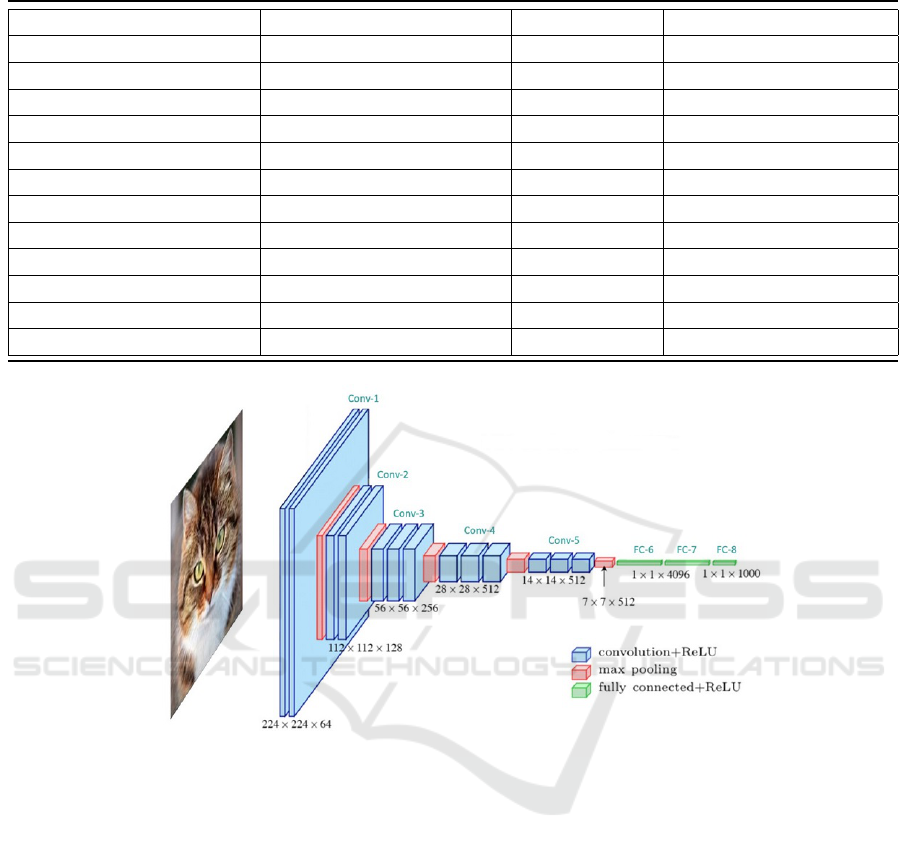
Table 1: Main Features of Related Works.

Work Classiﬁcation Accuracy Quantization Number of Classiﬁers

(Babic et al., 2016) 0.89 No 2

(Stojni

c et al., 2018) 0.92 No 2

(Rodriguez et al., 2018) 0.96 No 8

(Sledevi

c, 2018) 0.94 No 3

(Yang and Collins, 2019) 0.93 No 2

(Ngo et al., 2021) 0.94 No 1

(Berkaya et al., 2021) 0.99 No 10

(Monteiro et al., 2021) 0.99 No 9

(Benahmed et al., 2022) 0.99 No 2

(Pat-Cetina et al., 2023) 0.99 No 2

(Nguyen et al., 2024) 0.98 No 3

(This Work) 0.99 Yes 14

Figure 1: Vgg-16 CNN Architecture.

of models and reducing energy consumption, mak-

ing it more suitable for use in devices edge devices

such as smartphones and devices used in the inter-

net of things (IoT) and which have less storage and

processing capacity and a limited amount of energy

in battery-powered devices. Due to these character-

istics of reducing the model size and running infer-

ence faster, can mean the difference between a model

achieving quality of service goals or adapting to the

constraints often imposed by a mobile device (Raghu-

raman Krishnamoorthi and Weidman, 2024). When

using quantization we must consider some factors

such as:

• Loss of accuracy: When the problem involved is

complex, quantization can result in a loss of accu-

racy introduced by the approximations made by

the quantization process;

• Approach used: There are several forms of quan-

tization and it can be carried out in different layers

and with different parameters, making it possible

to investigate the best scenarios.

3.3 Transfer Learning

Transfer learning is a machine learning technique

where a model trained to solve a speciﬁc task is reused

as a starting point to address a different but related

task. This approach leverages the knowledge gained

from one problem to improve performance or efﬁ-

ciency in another, often reducing the need for large

datasets and extensive computational resources.

The core idea of transfer learning lies in using pre-

trained models, which are initially trained on large

datasets, typically for general-purpose tasks like ob-

ject recognition in images. These models learn to cap-

ture basic features (such as edges and textures) and

Inﬂuence of Quantization of Convolutional Neural Networks on Image Classiﬁcation of Pollen-Bearing Bees

151

more complex patterns (such as shapes and semantic

meanings). They can then be ﬁne-tuned for a spe-

ciﬁc task in a process called ﬁne-tuning. During this

process, some layers of the model may remain ﬁxed,

while others are retrained to learn new, task-speciﬁc

features.

This technique is particularly useful when the

available data for the target task is limited or when the

computational cost of training a model from scratch is

too high. Furthermore, transfer learning is most effec-

tive when the tasks share similar feature representa-

tions, such as in various image recognition problems.

The main beneﬁts of this approach include faster

training times, improved model performance with less

data, and reduced computational resource require-

ments. Transfer learning is, therefore, a powerful tool

that allows machine learning practitioners to leverage

pre-trained models to tackle new challenges more efﬁ-

ciently. Typical applications include computer vision,

where models like YOLO and VGG are ﬁne-tuned for

tasks such as image analysis or object detection.

4 EXPERIMENTAL SETUP

4.1 Classiﬁers

In this work, fourteen different classiﬁcation models

were used using the deep learning approach to clas-

sify images of bees with and without pollen. Af-

ter surveying related work, fourteen different clas-

siﬁcation models were selected. Most of the mod-

els had not yet been tested at the time of this re-

search on this bee classiﬁcation problem, such as

the models: efﬁcientnet b0, efﬁcientnet b1, mnas-

net0 5, mnasnet1 3, mobilenet v2, regnet x 400mf,

regnet y 1 6gf, regnet y 400mf and regnet y 800mf.

Other models such as: alexnet, googlenet and vgg16

were selected based on the good results obtained in

other works.

4.2 Conﬁgurations

To carry out the experimental tests on the fourteen

CNN architectures adopted, the transfer learning tech-

nique was used in which the models are previously

trained on a database and provide a set of weights that

serve as a starting point for more speciﬁc sets of im-

ages. The images from the database used were nor-

malized and resized according to the speciﬁcations of

each model.

The images were divided into 75% for training

and 25% for testing and the training images are ran-

domly rotated horizontally in training. The batch size

used was 16, the learning rate was 0.0003, the opti-

mizer used was Root Mean Square Propagation (RM-

Sprop) and the number of epochs speciﬁed was 15.

The training was carried out on the Google Colab

platform using Python 3 and Google Compute En-

gine backend (GPU) with 12.7GB of RAM and 15GB

GPU RAM. At the time of carrying out this work, Py-

torch does not allow running inference on quantized

models using a GPU (Raghuraman Krishnamoorthi

and Weidman, 2024). Therefore, the inference tests

shown in table 2 in all its variations (ﬂoat32, ﬂoat16

and int8) were carried out on a Ryzen 4600G CPU

with 16GB of RAM. For coding, the Pytorch libraries

were used for the image classiﬁcation part and sklearn

for calculating the metrics.

In carrying out this work, the dynamic quantiza-

tion technique was used. After training, each of the 14

selected models were converted into quantized mod-

els. The models were quantized using the 16-bit ﬂoat

and 8-bit int types resulting in 42 tests performed.

4.3 Performance Metrics

To evaluate the classiﬁcation performance in the bee

database, several metrics were used based on the con-

fusion matrix as shown in Figure 2.

True Positive (TP): Number of images of bees

with pollen that were correctly classiﬁed as images

of bees carrying pollen.

False Negative (FN): Number of images of bees

with pollen that were incorrectly classiﬁed as images

of non-pollen-bearing bees.

False Positive (FP): Number of images of bees

without pollen that were incorrectly classiﬁed as im-

ages of bees carrying pollen.

True Negative (TN): Number of images of pollen-

free bees that were correctly classiﬁed as images of

non-pollen-bearing bees.

The metrics calculated according to the confusion

matrix were as follows:

Accuracy: Calculates the general probability of

success. This way, accuracy considers the successes

of the two classes, pollen-carrying bees and non-

pollen-carrying bees, under all errors and successes.

Precision: Calculates the proportion of predic-

tions from the positive image class, which in the case

studied correspond to non-pollen-carrying bees, how

many actually were from non-pollen-carrying bees.

Recall: Calculates the probability of correctly

identifying the positive image class, that is, of the im-

ages of non-pollen-carrying bees as many as were cor-

rectly predicted.

F1-score: Takes stock comparing precision and re-

call. It is calculated through the harmonic mean of

ICEIS 2025 - 27th International Conference on Enterprise Information Systems

152

Figure 2: Example of Confusion Matrix for classiﬁcation of Pollen-bearing Bees and non Pollen-bearing Bees.

precision and recall, providing a result that balances

these two quantities.

False positive rate (FPR): Calculates the propor-

tion of negative classes, which in the case studied cor-

respond to pollen-carrying bees, which are incorrectly

predicted as images of non-pollen-carrying bees.

The formulas for calculating accuracy, precision,

recall, f1-score and FPR are illustrated respectively in

equations 1, 2, 3, 4 and 5.

Accuracy =

T P + T N

T P + T N + FP + FN

(1)

Precision =

T P

T P + FP

(2)

Recall =

T P

T P + FN

(3)

F1-score =

2 × Recall × Precision

Recall + Precision

(4)

FPR =

FP + T N

(5)

4.4 Dataset

The dataset used in this work was created in 2018 by

(Rodriguez et al., 2018). This dataset contains high-

resolution images (180 × 300) of pollen-carrying and

non-pollen-carrying bees and their respective labels,

as shown in Figure 3. It contains a total of 714 bees

annotated images, with 369 labeled as pollen bearing

and 345 as not pollen. It is important to highlight that

it was the ﬁrst public dataset using natural light, good

resolution imaging and manual annotation of the bee

position and orientation

. Following (Le et al., 2023),

We removed some images that were wrongly labeled.

To reduce the imbalance between classes and enhance

the effect of horizontal rotation on the images, 7 train-

ing images from the class without pollen were copied,

resulting in a dataset with 715 images, 365 images la-

beled as Pollen bearing and 350 as Not Pollen.

5 EXPERIMENTAL RESULTS

The classiﬁcation results are summarized in Table 2.

To maintain a compact presentation, only the model

https://github.com/piperod/PollenDataset

Figure 3: Examples of images of bees: in the ﬁrst line bees

with pollen and in the second without pollen.

names are included, as all three variations tested

(ﬂoat32, ﬂoat16, and int8) yielded identical values

in terms of accuracy, precision, recall, F1-score, and

false positive rate (FPR). For instance, the AlexNet

model consistently achieved an accuracy of 0.98 and

a precision of 0.99 across all its variations (ﬂoat32,

ﬂoat16, and int8). Then, we conclude that quantiza-

tion did not change the values of these metrics.

Analyzing Table 2, we can observe that the eval-

uated models achieved accuracy values ranging from

0.72 to 0.99. The highest accuracy was obtained by

the regnet y 400mf and mnasnet1 3 models, while

the lowest accuracy was observed in the mnasnet0 5

model. Regarding the precision metric, the evalu-

ated models achieved values ranging from 0.99 to 1.

Note that the worst model for the precison metric was

AlexNet, which achieved a value of 0.99. All other

models achieved a precision value of 1. Recall values

varied between 0.63 and 0.99. The regnet y 400mf

and mnasnet1 3 models achieved the highest recall of

0.99, whereas the mnasnet0 5 model had the lowest

recall of 0.63. The F1-scores of the models ranged

from 0.78 to 0.99. The regnet y 400mf and mnas-

net1 3 models achieved the highest F1-scores of 0.99,

while the lowest score of 0.78 was recorded by the

mnasnet0 5 model. Finally, the false positive rate

(FPR) values ranged from 0 to 0.01. Most mod-

els achieved an FPR of 0, with the exception of the

Inﬂuence of Quantization of Convolutional Neural Networks on Image Classiﬁcation of Pollen-Bearing Bees

153

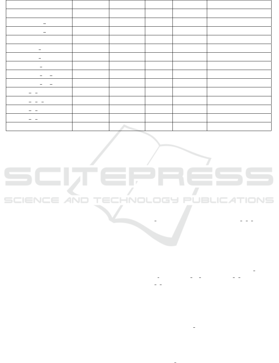
Table 2: Classiﬁcation results. To make the table more compact, only the model name was included, as the 3 variations tested

(ﬂoat32, ﬂoat16 and int8) had the same results.

Model Accuracy Precision Recall F1-score False Positive Rate

alexnet 0.98 0.99 0.98 0.98 0.01

efﬁcientnet b0 0.98 1 0.96 0.98 0

efﬁcientnet b1 0.95 1 0.91 0.96 0

googlenet 0.98 1 0.97 0.98 0

mnasnet0 5 0.72 1 0.63 0.78 0

mnasnet1 3 0.99 1 0.99 0.99 0

mobilenet v2 0.98 1 0.97 0.98 0

mobilenet v3 large 0.97 1 0.94 0.97 0

mobilenet v3 small 0.97 1 0.94 0.97 0

regnet x 400mf 0.95 1 0.91 0.96 0

regnet y 1 6gf 0.97 1 0.93 0.97 0

regnet y 400mf 0.99 1 0.99 0.99 0

regnet y 800mf 0.97 1 0.94 0.97 0

vgg16 0.98 1 0.97 0.98 0

alexnet model, which recorded the highest FPR value

of 0.01.

Table 3 presents the results of the 42 tests con-

ducted. In the ”Model´´ column, the original ﬂoat32

model appears ﬁrst, followed by the quantized mod-

els, which are identiﬁed by appending ”int8´´ or

”ﬂoat16´´ to the original model name to indicate their

respective quantization types. The ”Time Test´´ col-

umn represents the total time required by each model

to process the 176 test images, while the ”Time Test

Average´´ column displays the average time needed

to infer a single image. The ”Time Difference from

Original´´ column shows the percentage change in

inference time between the quantized models (ﬂoat16

or int8) and the original ﬂoat32 model. The ’Time

Test’ values shown in Table 3 show a trend as they

may vary between different executions as the machine

has several processes in parallel competing for CPU

use. The ”Size Difference Compared to the Origi-

nal´´ column provides the percentage difference in

model size between the original model and its quan-

tized variations. For the ”Time Difference from Orig-

inal´´ and ”Size Difference Compared to the Orig-

inal´´ columns, negative values signify reductions

relative to the original ﬂoat32 model. These reduc-

tions highlight the performance improvements and in-

creased efﬁciency achieved through quantization to

ﬂoat16 or int8.

The classiﬁcation time for the 176 images (time

test) across the models ranged from 2.3902 seconds to

41.6023 seconds. The time test average values, rep-

resenting the average time to classify a single image,

ranged from 0.0136 seconds to 0.2364 seconds.

5.1 Quantization Analysis

It is noteworthy that all models and their quantized

versions exhibited identical performance in terms of

accuracy, precision, recall, F1-score, and FPR met-

rics, as shown in Table 2. This consistent performance

may be attributed to the relatively simple nature of the

problem, as it involves binary classiﬁcation.

Regarding testing time, the majority of the evalu-

ated models showed improved performance with the

quantization process. However, two models, efﬁcient-

net b1 quantized to int8 and regnet y 1 6gf quan-

tized to int8, performed worse than their ﬂoat32

counterparts, being 3.33% and 5.2% slower, respec-

tively. These ﬁndings demonstrate that quantiza-

tion does not guarantee better inference times in all

cases. Still regarding the test time, most models

performed better when quantized to ﬂoat16. Six of

the evaluated models (alexnet, mnasnet0 5, mnas-

net1 3, mobilenet v3 small, regnet x 400mf and reg-

net y 400mf) obtained better results when quantized

to int8. Notably, the best result was obtained with

alexnet quantized to int8, achieving a test time of

2.3902 seconds, which was the shortest inference time

among all models analyzed. On the other hand, the

worst inference time, 41.6023 seconds, was obtained

by the efﬁcientnet b1 model quantized to int8, fur-

ther illustrating that int8 quantization does not guar-

antee optimal performance. The models that beneﬁted

the most in terms of reduced testing time were from

the efﬁcientnet family when quantized to ﬂoat16. The

efﬁcientnet b0 model achieved the largest percentage

reduction, with a time decrease of 64.25%, followed

ICEIS 2025 - 27th International Conference on Enterprise Information Systems

154

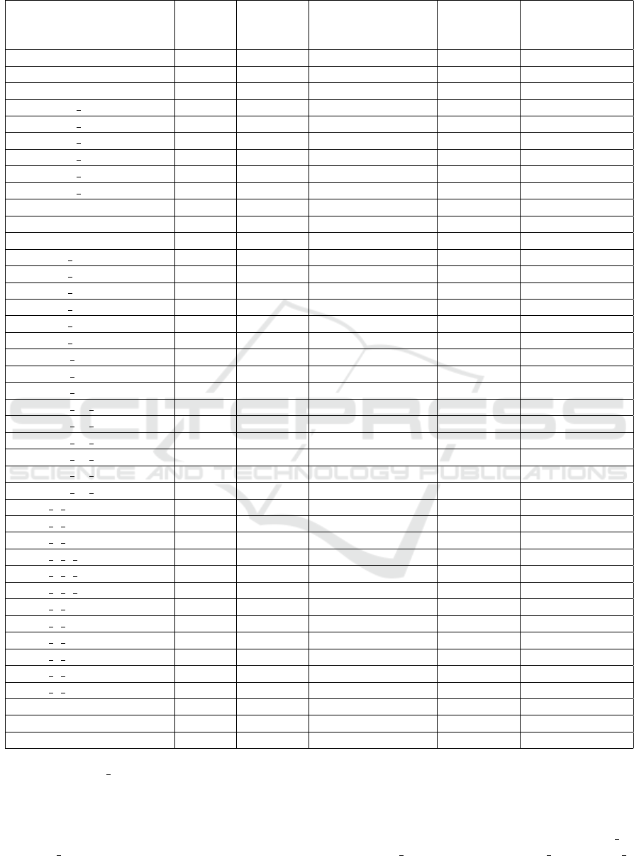
Table 3: Time and size results.

Model

Time

Test (s)

Time Test

Average

Difference in

Time Compared

to the Original in %

Model

Size (kb)

Size Difference

Compared to

the Original in %

alexnet 4.3961 0.025 - 228037.87 -

alexnet int8 2.3902 0.0136 -45.63 64449.816 -71.7372

alexnet ﬂoat16 3.1421 0.0179 -28.52 228039.832 0.0009

efﬁcientnet b0 32.7901 0.1863 - 16335.098 -

efﬁcientnet b0 int8 27.1998 0.1545 -17.05 16332.122 -0.0182

efﬁcientnet b0 ﬂoat16 11.7209 0.0666 -64.25 16335.898 0.0049

efﬁcientnet b1 40.2625 0.2288 - 26491.898 -

efﬁcientnet b1 int8 41.6023 0.2364 3.33 26488.922 -0.0112

efﬁcientnet b1 ﬂoat16 14.4434 0.0821 -64.13 26492.634 0.0028

googlenet 9.7841 0.0556 - 22581.394 -

googlenet int8 9.623 0.0547 -1.65 22579.174 -0.0098

googlenet ﬂoat16 9.6046 0.0546 -1.83 22582.182 0.0035

mnasnet0 5 3.9081 0.0222 - 3942.436 -

mnasnet0 5 int8 3.6046 0.0205 -7.77 3939.45 -0.0757

mnasnet0 5 ﬂoat16 3.756 0.0213 -3.89 3943.162 0.0184

mnasnet1 3 7.1776 0.0408 - 20309.476 -

mnasnet1 3 int8 6.6175 0.0376 -7.8 20306.49 -0.0147

mnasnet1 3 ﬂoat16 7.0074 0.0398 -2.37 20310.202 0.0036

mobilenet v2 16.4975 0.0937 - 9145.312 -

mobilenet v2 int8 13.8495 0.0787 -16.05 9142.394 -0.03

mobilenet v2 ﬂoat16 9.0975 0.0517 -44.86 9146.106 0.01

mobilenet v3 large 6.6647 0.0379 - 17020.654 -

mobilenet v3 large int8 6.461 0.0367 -3.06 13332.09 -21.67

mobilenet v3 large ﬂoat16 6.1732 0.0351 -7.38 17022.202 0.01

mobilenet v3 small 3.6438 0.0207 - 6210.85 -

mobilenet v3 small int8 3.2061 0.0182 -12.01 4439.982 -28.51

mobilenet v3 small ﬂoat16 3.5005 0.0199 -3.93 6212.398 0.02

regnet x 400mf 5.2535 0.0298 - 20694.986 -

regnet x 400mf int8 4.9288 0.028 -6.18 20694.632 -0.0017

regnet x 400mf ﬂoat16 5.1895 0.0295 -1.22 20695.72 0.0035

regnet y 1 6gf 14.5459 0.0826 - 41708.004 -

regnet y 1 6gf int8 15.3027 0.0869 5.2 41706.178 -0.0044

regnet y 1 6gf ﬂoat16 13.0503 0.0741 -10.28 41708.738 0.0018

regnet y 400mf 6.6522 0.0378 - 15867.638 -

regnet y 400mf int8 5.6538 0.0321 -15.01 15867.156 -0.003

regnet y 400mf ﬂoat16 5.972 0.0339 -10.23 15868.372 0.0046

regnet y 800mf 7.7305 0.0439 - 22846.754 -

regnet y 800mf int8 7.7032 0.0438 -0.35 22845.248 -0.0066

regnet y 800mf ﬂoat16 6.7945 0.0386 -12.11 22847.488 0.0032

vgg16 31.9778 0.1817 - 537069.974 -

vgg16 int8 27.3269 0.1553 -14.54 178447.028 -66.774

vgg16 ﬂoat16 24.7501 0.1406 -22.6 537072.18 0.0004

by the efﬁcientnet b1 model, which saw a reduction

of 64.13%. These results highlight the signiﬁcant per-

formance improvements that ﬂoat16 quantization can

offer, particularly for certain model architectures.

Regarding model sizes, the smallest model was

mnasnet0 5, with a size of 3942.436 KB. How-

ever, this model also had the poorest performance

in terms of accuracy, precision, recall, F1-score, and

FPR. All models experienced size reductions when

quantized to int8 compared to their ﬂoat32 counter-

parts. For some models, including efﬁcientnet b0,

efﬁcientnet b1, googlenet, mnasnet0 5, mnasnet1 3,

Inﬂuence of Quantization of Convolutional Neural Networks on Image Classiﬁcation of Pollen-Bearing Bees

155

mobilenet v2, regnet x 400mf, regnet y 1 6gf, reg-

net y 400mf, and regnet y 800mf, the reductions

were minimal, with decreases of less than 0.01%. In

contrast, other models achieved signiﬁcant size re-

ductions with int8 quantization. Notably, the vgg16

model saw a size reduction of 66.774%, while the

alexnet model achieved the largest reduction, with a

71.7372% decrease compared to its original size. On

the other hand, quantization to ﬂoat16 resulted in a

slight increase in size across all models, with the in-

crease being less than 0.01%. These results demon-

strate that while int8 quantization can be highly effec-

tive in reducing model sizes, ﬂoat16 quantization may

lead to negligible size increases.

Overall, the model that achieved the best results

in the quantization process was AlexNet. Not only

did it maintain its performance in terms of accuracy,

but when quantized to int8, it also obtained the short-

est inference time among all the evaluated models.

Furthermore, it demonstrated substantial reductions

in both inference time (-45.63%) and model size (-

71.7372%), making it a standout performer in the

quantization analysis.

6 CONCLUSIONS

In this study, we analyze fouteen deep convolutional

neural network models for the classiﬁcation of bees

carrying pollen versus those not carrying pollen in

images taken at the hive entrance. Furthermore,

we investigate the effects of the quantization pro-

cess on these models’ performance. Quantization

can reduce inference time and model size by using

lower-precision formats for calculations and data stor-

age. Considering the frequent use of embedded sys-

tems for image acquisition, which are often limited

in memory and computational resources, quantized

models provide notable advantages. Our results show

that, for the evaluated dataset, it is possible to improve

inference time and/or model size without compromis-

ing key performance metrics such as accuracy, preci-

sion, recall, F1-score, and false positive rate (FPR).

Considering all the results obtained, no single

model excels in all aspects compared to the others.

Therefore, setting priorities is crucial in an imple-

mentation project, and testing the available options is

essential to make a choice that best aligns with the

speciﬁc requirements of the problem. If the prior-

ity lies in performance metrics such as accuracy, pre-

cision, recall, F1-score, and FPR, the recommended

choices would be mnasnet1 3 quantized to int8 or reg-

net y 400mf quantized to int8. Among these, reg-

net y 400mf has a slight edge due to better inference

time and smaller model size. For applications where

inference time is the critical factor, alexnet quantized

to int8 stands out as the best choice. It achieved the

shortest inference time while maintaining strong over-

all performance, with an accuracy of 0.98. If model

size is the priority, the smallest model was mnas-

net0 5 quantized to int8. However, its low accuracy

of 0.72 makes it a less ideal choice. A better alterna-

tive might be mobilenet v3 small quantized to int8,

which offers a reduced size (4439.982 KB compared

to 3942.436 KB for mnasnet0 5) while achieving a

much higher accuracy of 0.97. This balance of size

and accuracy makes it a more practical option for sce-

narios where both factors are important.

As future work, we plan to evaluate additional

datasets. We anticipate that conducting more exten-

sive tests will provide deeper insights into the limi-

tations of the models, ultimately leading to improved

classiﬁcation performance. Besides, we plan to com-

bine different CNNs in order to further improve the

performance.

ACKNOWLEDGMENTS

This work was partially funded by Lenovo as part of

its R&D investment under the Information Technol-

ogy Law. The authors would like to thank LSBD/UFC

for the partial funding of this research.

REFERENCES

Babic, Z., Pilipovic, R., Risojevic, V., and Mirjanic, G.

(2016). Pollen bearing honey bee detection in hive

entrance video recorded by remote embedded system

for pollination monitoring. ISPRS Annals of the Pho-

togrammetry, Remote Sensing and Spatial Informa-

tion Sciences, 3:51–57.

Benahmed, H. K., Bensaad, M. L., and Chaib, N. (2022).

Detection and tracking of honeybees using yolo and

strongsort. In 2022 2nd International Conference on

Electronic and Electrical Engineering and Intelligent

System (ICE3IS), pages 18–23.

Berkaya, S. K., Gunal, E. S., and Gunal, S. (2021). Deep

learning-based classiﬁcation models for beehive mon-

itoring. Ecological Informatics, 64:101353.

Bilik, S., Zemcik, T., Kratochvila, L., Ricanek, D., Richter,

M., Zambanini, S., and Horak, K. (2024). Machine

learning and computer vision techniques in continu-

ous beehive monitoring applications: A survey. Com-

puters and Electronics in Agriculture, 217:108560.

IBM Contributors (2024). What are convolutional

neural networks? https://www.ibm.com/think/

topics/convolutional-neural-networks.

ICEIS 2025 - 27th International Conference on Enterprise Information Systems

156

Le, T.-N., Thi-Thu-Hong, P., Nguyen, H.-D., Thi-Lan, L.,

et al. (2023). A novel convolutional neural network

architecture for pollen-bearing honeybee recognition.

International Journal of Advanced Computer Science

and Applications, 14(8).

LearnOpenCV (2024). Understanding convolutional neural

networks (cnn).

Monteiro, F. C., Pinto, C. M., and Ruﬁno, J. (2021). To-

wards precise recognition of pollen bearing bees by

convolutional neural networks. In Iberoamerican

Congress on Pattern Recognition. Springer.

Ngo, T. N., Rustia, D. J. A., Yang, E.-C., and Lin, T.-T.

(2021). Automated monitoring and analyses of honey

bee pollen foraging behavior using a deep learning-

based imaging system. Computers and Electronics in

Agriculture, 187:106239.

Nguyen, D., Le, T., Phung, T., Nguyen, D., Nguyen, H.,

Pham, H., Phan, T., Vu, H., and Le, T. (2024). Improv-

ing pollen-bearing honey bee detection from videos

captured at hive entrance by combining deep learning

and handling imbalance techniques. Ecol. Informat-

ics, 82:102744.

Pat-Cetina, J. E., Orozco-del Castillo, M. G., L

opez-Puerto,

K. A., Bermejo-Sabbagh, C., and Cuevas-Cuevas,

N. L. (2023). Recognition of pollen-carrying bees us-

ing convolutional neural networks and digital image

processing techniques. In Mata-Rivera, M. F., Zagal-

Flores, R., and Barria-Huidobro, C., editors, Telemat-

ics and Computing, pages 253–269, Cham. Springer

Nature Switzerland.

PyTorch Contributors (2023). Introduction to quantization.

https://pytorch.org/docs/stable/quantization.html.

Raghuraman Krishnamoorthi, James Reed, M. N. C. G.

and Weidman, S. (2024). Introduction to quan-

tization on pytorch. https://pytorch.org/blog/

introduction-to-quantization-on-pytorch/.

Rodriguez, I. F., Megret, R., Acuna, E., Agosto-Rivera,

J. L., and Giray, T. (2018). Recognition of pollen-

bearing bees from video using convolutional neural

network. In 2018 IEEE winter conference on appli-

cations of computer vision (WACV), pages 314–322.

IEEE.

Rohafauzi, S., Kassim, M., Ja’afar, H., Rustam, I., and

Miskon, M. T. (2024). A review on internet of things-

based stingless bee’s honey production with image de-

tection framework. International Journal of Electri-

cal and Computer Engineering (IJECE), 14(2):2282–

2292.

Sledevi

c, T. (2018). The application of convolutional neu-

ral network for pollen bearing bee classiﬁcation. In

2018 IEEE 6th Workshop on Advances in Information,

Electronic and Electrical Engineering (AIEEE), pages

1–4. IEEE.

Stojni

c, V., Risojevi

c, V., and Pilipovi

c, R. (2018). De-

tection of pollen bearing honey bees in hive en-

trance images. In 2018 17th International Symposium

INFOTEH-JAHORINA (INFOTEH), pages 1–4. IEEE.

Wu, H., Judd, P., Zhang, X., Isaev, M., and Micikevicius,

P. (2020). Integer quantization for deep learning in-

ference: Principles and empirical evaluation. arXiv

preprint arXiv:2004.09602.

Yang, C. and Collins, J. (2019). Deep learning for pollen

sac detection and measurement on honeybee monitor-

ing video. In 2019 International Conference on Image

and Vision Computing New Zealand (IVCNZ), pages

1–6. IEEE.

Zacepins, A., Brusbardis, V., Meitalovs, J., and Stalidzans,

E. (2015). Challenges in the development of precision

beekeeping. Biosystems Engineering, 130:60–71.

Inﬂuence of Quantization of Convolutional Neural Networks on Image Classiﬁcation of Pollen-Bearing Bees

157