A Predictive Greenhouse Digital Twin for Controlled Environment
Agriculture
Abdellah Islam Kafi
a
, Antonio P. Sanfilippo
b
, Raka Jovanovic
c
and Sa’d Abdel-Halim Shannak
d
Qatar Environment and Energy Research Institute, Hamad Bin Khalifa University, Doah, Qatar
Keywords:
Digital Twin, Controlled Environment Agriculture, Time Series Forecasting, Machine Learning, Crop Yield
Modeling, Edge Implementation.
Abstract:
Controlled environment agriculture offers significant advantages for the efficient use of resources in food
production, especially in hot desert climate regions due to the scarcity of arable land and water. However,
farming practices such as hydroponics and aquaponics have high energy requirements for temperature con-
trol and present higher operational complexity when compared to traditional forms of farming. This study
describes a Predictive Greenhouse Digital Twin (PGDT) that addresses these challenges through a dynamic
crop yield assessment. The PGDT uses greenhouse measurements gathered through an IoT sensor network
and a regression approach to multivariate time series forecasting to develop a model capable of predicting final
crop yield as a function of the gathered measurements at any point in the crop cycle. The performance of the
PGDT is evaluated with reference to forecasting algorithms based on deep and ensemble learning methods.
Overall, deep learning methods show superior performance, with Long short-term memory (LSTM) providing
a marginal advantage compared to Deep Neural networks (DNN). Furthermore, the models were deployed on
an edge device (a Raspberry Pi-based gateway), where DNN demonstrated faster inference while delivering
performance better than LSTM.
1 INTRODUCTION
As climate change keeps driving desertification
through land degradation (Sivakumar, 2007) (Huang
et al., 2020), food crop production becomes increas-
ingly challenging, especially in hot desert climate re-
gions due to the scarcity of water and arable land.
For example, only 2.6% of Qatar’s land was allo-
cated to food production in 2019 (Planning and Au-
thority, 2021) and only a small portion of the al-
ready scarce ground water is suitable for crop irriga-
tion due to the presence of total dissolved solids con-
centration levels which are not suitable for food crops
(Sanfilippo et al., 2024). Hydroponic and aquaponic
farming alleviate these impediments through soil-less
farming and significant reduction of water use but
have high energy requirements for temperature con-
trol and present higher operational complexity when
a
https://orcid.org/0000-0001-8523-3492
b
https://orcid.org/0000-0001-7097-4562
c
https://orcid.org/0000-0001-8167-1516
d
https://orcid.org/0000-0002-6842-7479
compared to traditional forms of farming (Sanfilippo
et al., 2024). Both problems can be addressed through
the development of a Predictive Greenhouse Digital
Twin (PGDT) that can help identify the most efficient,
profitable and sustainable use of resources in achiev-
ing the highest crop yields.
The PGDT presented in this study provides the
basis for the automatic identification of economically
sustainability in indoor farming through dynamic as-
sessment of crop yield at any stage during the produc-
tion cycle. The PGDT uses greenhouse measurements
from a IoT sensor network and a regression approach
to multivariate time series forecasting to provide a
model capable to predict crop productivity as a func-
tion of the collected measurements. The integration of
the PGDT with multi-objective optimization and tech-
noeconomic analysis components can then be used to
identify ideal trade-offs in the use of resources such as
electricity, water and nutrients, and evaluate the eco-
nomic sustainability of the ensuing trade-off scenar-
ios as discussed in (Sanfilippo et al., 2024). The per-
formance of the PGDT is evaluated with reference to
three forecasting algorithms, two based on deep learn-
980
Kafi, A. I., Sanfilippo, A. P., Jovanovic, R. and Shannak, S. A.-H.
A Predictive Greenhouse Digital Twin for Controlled Environment Agriculture.
DOI: 10.5220/0013479900003929
Paper published under CC license (CC BY-NC-ND 4.0)
In Proceedings of the 27th International Conference on Enterprise Information Systems (ICEIS 2025) - Volume 1, pages 980-987
ISBN: 978-989-758-749-8; ISSN: 2184-4992
Proceedings Copyright © 2025 by SCITEPRESS – Science and Technology Publications, Lda.

ing methods (Deep Neural networks (DNN) and Long
short-term memory (LSTM)) and the third based on
the eXtreme Gradient Boosting algorithm (XGBoost).
The paper is structured into five sections. First,
a review of the background literature on crop yield
modeling is provided to highlight the contribution of
the present study. Then the data used in this study
and their sources are discussed. Next, the methodol-
ogy used in the development of the PGDT is described
and finally the results are presented. The paper con-
cludes with a discussion of next steps with specific
reference to integration with the multi-objective opti-
mization and techno-economic analysis components.
2 BACKGROUND
Work on PGDTs as predictive models of greenhouse
productivity can be grouped into two main categories
according to whether first principle models or ma-
chine learning algorithms are used.
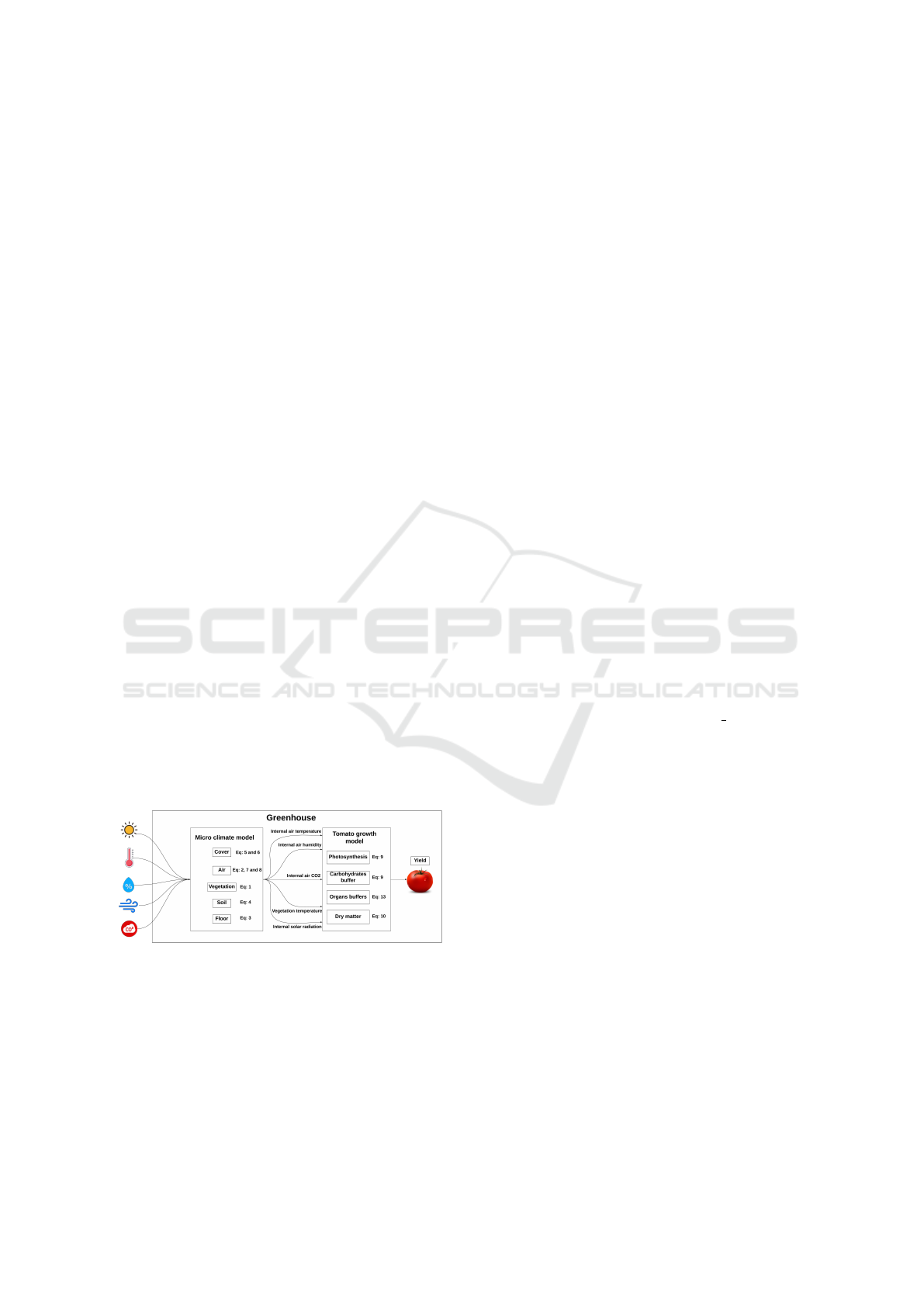
An example of PGDT based on first principle
models is presented in (Sanfilippo et al., 2024) us-
ing the greenhouse micro-climate and tomato yield
models developed in (Vanthoor et al., 2011b) and
(Vanthoor et al., 2011a). The greenhouse micro-
climate includes equations that compute the impact
of factors relative to climate control in the green-
house such as the insulation properties of the plastic
sheeting covering the greenhouse, ventilation, the ab-
sorption of near-infrared radiation, plant transpiration
rate, and fluxes generated by the plants’ canopy activ-
ity. The tomato growth model employs a shared car-
bohydrate buffer that handles the distribution to plant
organs and is primarily influenced the micro-climate
model, as shown in Figure 1.
Figure 1: Example of PGDT based on a first principles
model (Sanfilippo et al., 2024).
Most PGDTs based on machine learning make use
of neural network algorithms. One of the earliest
studies (Ehret et al., 2011) provides a neural network
model of greenhouse tomato yield, growth and water
use from automated crop monitoring data. The study
described in (Qaddoum et al., 2013) used fuzzy neural
networks to model tomato yield. The authors in (Alh-
naity et al., 2019) make use of a long short-term mem-
ory neural network algorithm to model plant growth
in greenhouses and show that the model developed
outperforms support vector regression and random
forest algorithms. The authors in (Gong et al., 2021)
present a greenhouse crop yield prediction model that
combines temporal convolutional and recurrent neu-
ral networks and rivals traditional machine learning
approaches such as linear regression, random for-
est, support vector regression, decision tree, gradient
boosting, and multi-layers artificial neural network.
These studies all represent significant advanced in
modeling crop growth in a greenhouse environment.
Our study contributes to this endeavor through the
comparison of deep learning algorithms with the eX-
treme Gradient Boosting algorithm (XGBoost).
3 DATA
The data used in this study include meteorolog-
ical measurements outside the greenhouse moni-
tored through the National Solar Radiation Database
(NSRD) (https://nsrdb.nrel.gov) and measurements
from a hydroponic tomato greenhouse at the Agrico
Agricultural Development (https://agrico.qa). Green-
house measurements were gathered through a net-
work of IoT sensors installed in the hydroponic
tomato greenhouse throughout a full tomato growth
cycle, early November 2023 through the end of May
2024. These include electrical soil conductivity (EC),
luminosity (LUX), soil temperature (S TEMP), rela-
tive humidity (RH), air temperature (TEMP), pH, and
harvest quantities, as shown in Tables I and II. Har-
vest quantities were manually recorded and provide
the key indication of crop yield. For additional details
on the greenhouse characteristics and the IoT sensor
network see (Sanfilippo et al., 2024).
4 METHODOLOGY
The primary objective of this study is to assess and
compare the performance of three distinct forecasting
algorithms, DNN, LSTM, and XGBoost, in predicting
crop yield. A methodical approach was employed for
data collection, preprocessing, model development,
training procedures, and performance evaluation. The
most adequate models were chosen for implementa-
tion on an edge device to enable immediate yield fore-
casting in the greenhouse environment. The approach
included transforming the trained models into com-
pact formats appropriate for edge deployment and uti-
lizing quantization methods to minimize the models’
A Predictive Greenhouse Digital Twin for Controlled Environment Agriculture
981

memory usage and inference delay. The implementa-
tion setup was integrated with the existing IoT sensor
network, allowing seamless data flow.
4.1 DNN, LSTM and XGBoost
The architecture of DNNs (Sze et al., 2017) comprises
input, hidden and output layers. The input layer re-
ceives data. The hidden layers consist of intercon-
nected nodes where data inputs are associated with
weights. Each node computes the weighted sum of
its inputs and passes the results through an activation
function. Activated nodes are summed and passed
through to the output layer as predictions. During
training, forward and backward propagation steps op-
erate on training data records. In forward propaga-
tion, data are fed into the input layer, passed through
each hidden layer, and the network’s prediction is
generated from the final output layer. In backward
propagation, the network’s prediction is compared to
the observed value, the ensuing error is propagated
backward through the network layer by layer, and
the weights of the connections between nodes are ad-
justed using algorithms such as gradient descent to
minimize the error.
Differently from DNNs, an LSTM (Hochreiter,
1997) is structured as a network of cells. Each cell
contains a memory component, a forget gate, an input
gate and an output gate. After the LSTM cell receives
input data, the forget gate determines which informa-
tion from the previous step is to be discarded and the
input gate determines which new information should
be stored in memory. A new candidate value is com-
puted using the previous hidden state of the network,
the current input, and the input gate. The memory cell
is updated by combining the old memory cell content
with the new candidate value, weighted by the forget
gate and input gate values, respectively. The output
gate decides how much of the updated memory cell
content should be used to compute the output of the
cell. The final output of the LSTM cell is computed
by multiplying the output gate value with the updated
memory cell content.
In XGBoost (Chen and Guestrin, 2016) weak
learners are iteratively combined to minimize the en-
semble error. The model is initialized with a weak
learner, e.g., a decision stump model (Iba and Lang-
ley, 1992), which is evaluated on the reference dataset
to compute residuals using a loss function such as
the Mean Squared Error (MSE). Then, a new weak
learner is built that minimizes the loss function by
fitting the new weak learner to the dataset with the
objective of predicting both the first and second or-
der gradients of the loss function from the previous
Table 1: Harvest quantities time series sample.
Date Harvest Quantities (Kg.)
01/03/24 21
01/06/24 80
01/06/24 27
01/06/24 6
01/08/24 200
01/08/24 22
01/08/24 1
... ...
Table 2: Parameters measured in near real-time and aggre-
gated daily.
Date EC LUX S TEMP RH TEMP pH
06/11/23 0.7 8971.3 27.4 61.6 26.1 4.3
07/11/23 0.9 11891.4 26.7 61.1 26.4 4.9
... ... ... ... ... ... ...
weak learner. Finally, the ensemble model is updated
by adding a scaled version of the weak learner’s pre-
diction. This process is repeated until the optimal re-
sults are achieved and the final model is derived as the
weighted mean of all weak learners.
4.2 Data Wrangling
Before training and evaluating the DNN, LSTM and
XGBoost forecasting algorithms on the reference
dataset, the relation in time and frequency granular-
ity between the dependent variable, i.e., harvest quan-
tities, and the independent variables, i.e., EC, LUX,
S TEMP, RH, TEMP, and pH, in the dataset need to
be normalized. Harvest quantities are typically dis-
tributed unevenly through the production cycle, with
no output in the initial period of growth (i.e, early
November through early January in Qatar), multiple
or single collections of varying quantities in a sin-
gle day, and intervening days with no collection, as
shown in Table (1), while other parameters are mea-
sured in near real-time and aggregated daily as shown
in Table (2). So, while there are data points for every
day of the crop growth cycle (209 days) for the inde-
pendent variables, there are only 101 data points for
the dependent variable (i.e., harvest quantities) that
represent a total of 37 days taking into account days
of repeated harvesting.
We employed a sliding window technique to cap-
ture the temporal dependencies inherent in green-
house sensor data during feature engineering. This
method involves creating subsets of consecutive data
points, where each subset (or window) contains a
fixed number of time steps—in this case, eight days.
For every window, the corresponding input features
are aggregated to form a feature vector representing
the greenhouse’s state over the preceding eight-day
ICEIS 2025 - 27th International Conference on Enterprise Information Systems
982

period. Specifically, each window includes measure-
ments of EC, LUX, HUM, TEMP, YIELD, and the
number of days since the start of the plantation cycle.
The target variable for each window is the yield value
following the window period. By sliding this window
across the entire dataset, we generated many training
samples that enabled the models to learn patterns and
trends associated with crop growth and yield fluctua-
tions.
We employed a forward-filling method to assign
missing yield values to address the non-daily record-
ing of harvest quantities. Specifically, after a har-
vest event was recorded on a particular day, the cor-
responding yield value was carried forward and as-
signed to all subsequent days until the next harvest
day. This technique assures that the yield data stays
constant during periods without recorded harvests re-
flecting the real-world available information. By do-
ing so, the model can leverage the most recent yield
information when predicting future yields while min-
imizing the introduction of bias that could result from
arbitrary interpolation.
4.3 Training and Testing
We explore the architecture design and training pro-
cedures employed for each predictive model inte-
grated into the PGDT. We explore three distinct mod-
eling approaches: DNN, LSTM, and XGBoost. Each
model’s architecture, hyperparameter configurations,
and training methodologies are detailed to provide
a comprehensive understanding of their implementa-
tion characteristics. The training was conducted on
a Linux machine with an AMD Ryzen 7900 12-core
processor, an NVIDIA RTX 4070 GPU with 12 GB
of VRAM, and 32GB of DDR4 RAM. During train-
ing, the DNN and LSTM models were trained on the
GPU. The XGBoost model, implemented using the
XGBoost library, was trained on the CPU.
4.3.1 Deep Neural Network
The DNN model begins with an input layer that ac-
cepts data sequences with eight-time steps window
size. Subsequently, these multidimensional inputs are
flattened into a single vector to facilitate processing
by the dense layers. The DNN comprises two fully
connected hidden layers containing 256 neurons with
ReLU activation functions.
Training the DNN involved using the Adam op-
timizer with a learning rate 0.001, aiming to mini-
mize the Mean Squared Error (MSE) loss function.
The model was trained over 100 epochs with a batch
size of 32. TimeSeriesSplit with eight splits was em-
ployed for cross-validation, maintaining the chrono-
logical integrity of the time series data. Feature scal-
ing was performed using the MinMaxScaler, which
normalized the input features to a range between 0
and 1.
4.3.2 Long Short-Term Memory Network
The LSTM architecture begins with an input layer that
processes sequences of eight-time steps, each com-
prising six features similar to the DNN model. This
input is fed into a stack of LSTM layers, each con-
taining 256 memory units.
Each LSTM layer is equipped with dropout regu-
larization, although the current configuration sets the
dropout rate to 0.2 to control overfitting. The output
is a dense layer with a linear activation function, gen-
erating the predicted yield value.
Training the LSTM model utilized the Adam op-
timizer with a learning rate 0.001 and aimed to min-
imize the MSE loss function. The model was trained
for 100 epochs with a batch size of 32, TimeSeriesS-
plit with eight splits for cross-validation, and feature
scaling was similarly performed using the MinMaxS-
caler to normalize input features.
4.3.3 eXtreme Gradient Boosting
The XGBoost architecture was configured with a
learning rate of 0.1, 200 estimators, and a maximum
tree depth of six. Additionally, a subsample ratio of
0.8 was employed by randomly sampling 80% of the
training data for each tree. These hyperparameters
were selected to balance model complexity and gen-
eralization performance.
Training the XGBoost model involved fitting the
algorithm to the scaled training data using the Min-
MaxScaler to normalize the input features. The model
was trained over 200 boosting rounds with a learning
rate of 0.1, and it was optimized based on the gradient
of the loss function.
4.3.4 Evaluation Procedures
Each model’s performance was evaluated using key
metrics, including ,
Root Mean Squared Error (RMSE),
RMSE =
s
1
n
n
∑
i=1
(y
i
− ˆy
i
)
2
,
coefficient of determination (R
2
),
R
2
= 1 −
∑
n
i=1
(y
i
− ˆy
i
)
2
∑
n
i=1
(y
i
− ¯y)
2
,
and Mean Absolute Error (MAE),
MAE =
1
n
n
∑
i=1
|
y
i
− ˆy
i
|
.
A Predictive Greenhouse Digital Twin for Controlled Environment Agriculture
983

These metrics comprehensively assess each model’s
accuracy and generalization capability.
Furthermore, Mean Squared Error (MSE) is used
for the loss function and given by:
MSE =
1
n
n
∑
i=1
(y
i
− ˆy
i
)
2
,
Where:
• y
i
is the actual value,
• ˆy
i
is the predicted value,
• ¯y is the mean of the actual values,
• n is the number of observations.
5 RESULTS AND DISCUSSION
The experimental evaluation of the PGDT high-
lights different performance aspects among the DNN,
LSTM, and XGBoost models when forecasting green-
house tomato yields using the time series dataset de-
scribed in Section 3. This section presents an in-depth
discussion of the comparative performance of these
methods.
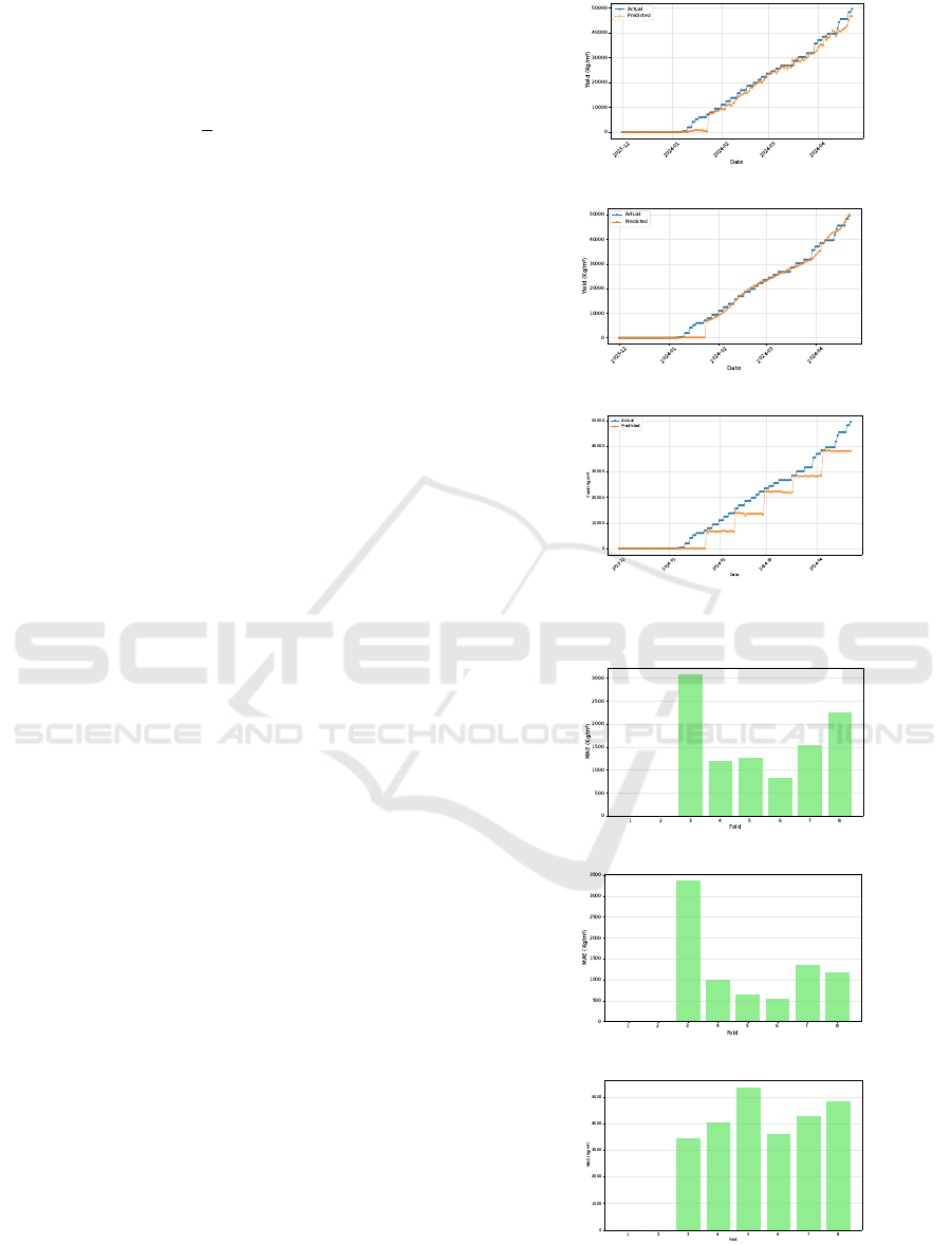
Figure 2 illustrates the actual versus predicted
yields for each model across the whole crop cycle,
catching both the beginning of fruit production and
the peak yield phase. Although all models exhibit a
general upward trend, their fidelity to ground truth
varies substantially, especially near the peak yield
phase.
Generally, Figure 2 demonstrates that DNN and
LSTM capture yield patterns. LSTM predictions
align more robustly with the ground truth observa-
tions. XGBoost, despite its overall ability to follow
the trend, always underestimates yield values. These
initial observations are further quantified in the sub-
sections below.
5.1 Metrics Analysis
Key metrics are employed to evaluate predictive ac-
curacy: MAE, RMSE, and (R
2
).
LSTM achieves the lowest MAE (1,007.39 kg/m
2
)
and RMSE (1,769.86 kg/m
2
), outperforming both
DNN and XGBoost. These lower error values indi-
cate that, on average, LSTM predictions remain closer
to actual harvest quantities and that more significant
prediction errors are less frequent.
Figure 3 shows the evolution of MAE across dif-
ferent folds, demonstrating the model stability with
various data subsets. LSTM consistently achieves
MAE values below 1,500 kg/m
2
across all folds, re-
flecting strong generalization. In contrast, the DNN
(a) DNN.
(b) LSTM.
(c) XGBoost.
Figure 2: Actual vs. predicted yields.
(a) DNN.
(b) LSTM.
(c) XGBoost.
Figure 3: MAE progression across folds.
ICEIS 2025 - 27th International Conference on Enterprise Information Systems
984

exhibits moderate fluctuations, with some folds rising
to nearly 1,800 kg/m
2
, implying sensitivity to partic-
ular training subsets. XGBoost, on the other hand,
displays significant fluctuations, with errors exceed-
ing 4,000 kg/m
2
in the later folds.
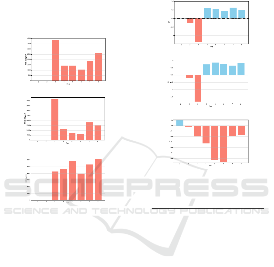
(a) DNN.
(b) LSTM.
(c) XGBoost.
Figure 4: RMSE trends across folds.
The RMSE results, plotted in Figure 4, follow the
MAE trends. DNN registers moderate RMSE fluc-
tuations, while LSTM retains relatively low RMSE
values across folds, showing its stable performance.
XGBoost’s errors are more than 5,000 kg/m
2
, high-
lighting the model’s low performance.
Evaluating the (R
2
) metric, LSTM attains the
highest score (0.986), slightly surpasses DNN
(0.984), and noticeably outperforms XGBoost
(0.916). Although the difference between LSTM and
DNN appears small, an inspection of the time series
predictions indicates a benefit during rapid transitions
and peak yield phases.
Figure 5 underscores that while DNN and LSTM
maintain relatively high R
2
values across folds, XG-
Boost occasionally drops into negative values, indi-
cating that the model can, in particular data splits, per-
form worse than a simple mean-based predictor.
(a) DNN.
(b) LSTM.
(c) XGBoost.
Figure 5: R
2
consistency. Negative values for XGBoost
indicate failed generalization.
Table 3: Comparative Model Performance Metrics.
Metric DNN LSTM XGBoost
MAE (kg/m
2
) 1,270.08 1,007.39 3,213.78
RMSE (kg/m
2
) 1,946.96 1,769.86 4,404.05
R
2
0.984 0.986 0.916
5.2 Edge Deployment
The final trained DNN and LSTM models were de-
ployed on an edge device, specifically a gateway
based on Raspberry Pi 4, to allow real-time yield pre-
diction at the greenhouse level. This edge deployment
guarantees localized processing of sensor data, reduc-
ing latency and dependence on cloud infrastructure
while maintaining data privacy. The TensorFlow Lite
framework was employed to convert the trained mod-
els into lightweight formats suitable for execution on
the microcontroller boards.
Both models were quantized to the Float16 preci-
sion format during conversion to reduce their size and
inference latency while maintaining nearly compara-
ble accuracy to their full-sized counterparts. Quan-
tization to Float16 reduces the memory footprint of
the models, making them favorable for edge devices.
After quantization, the size of the DNN model was
A Predictive Greenhouse Digital Twin for Controlled Environment Agriculture
985

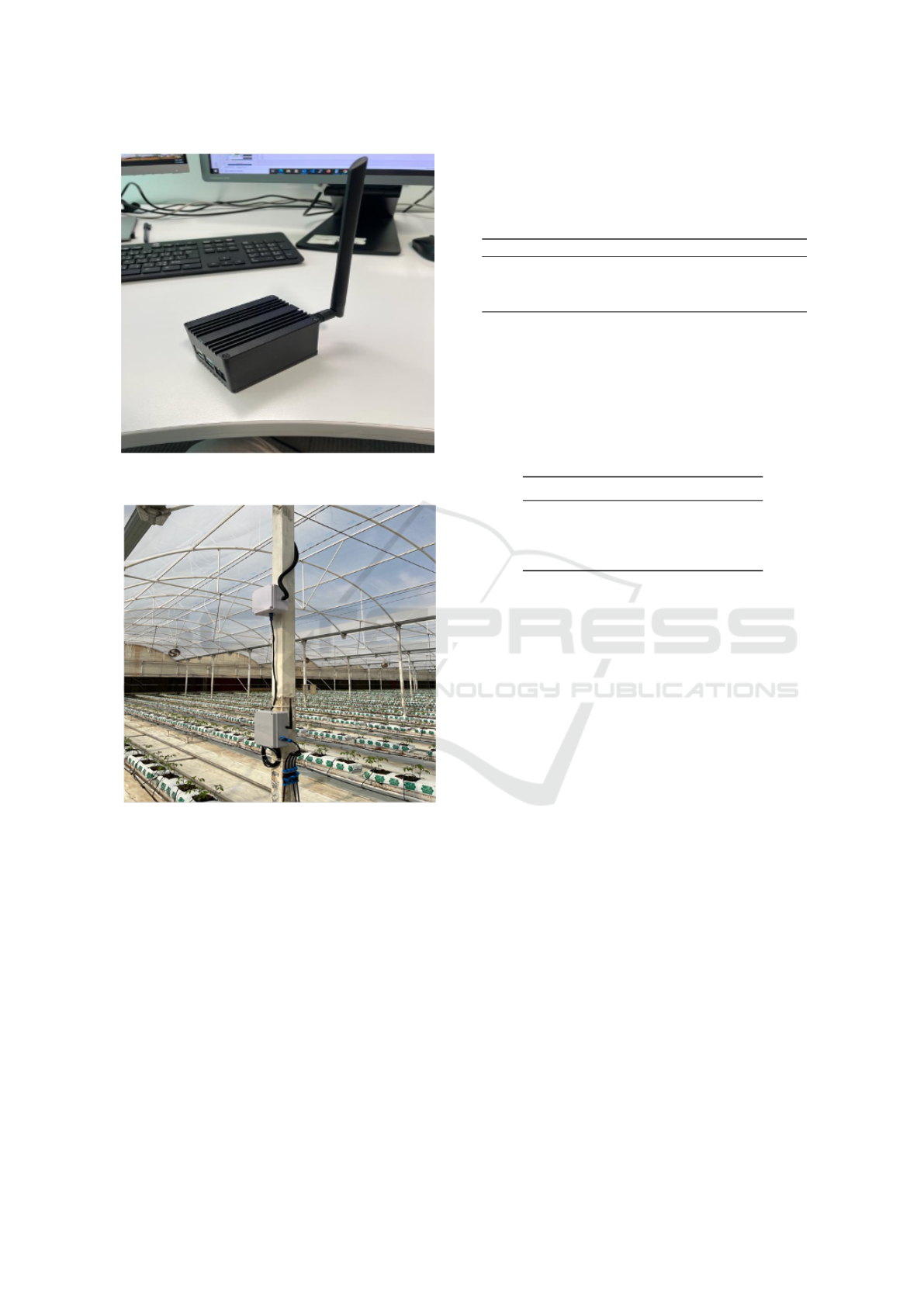
(a) The edge gateway device used to deploy the devel-
oped models.
(b) IoT sensor nodes installed inside the greenhouse for
data collection.
Figure 6: Edge deployment setup comprising the gateway
device and greenhouse sensor nodes.
reduced from 977 KB to just 160 KB and the LSTM
model from 3.3 MB to 549 KB.
Once deployed, the Float16 quantized models pro-
cessed real-time sensor data collected from the green-
house and provided yield predictions with average in-
ference times of approximately 0.000067 seconds for
the DNN and 0.005009 seconds for the LSTM on the
Raspberry Pi.
Table 4 summarizes the performance comparison
between the quantized and full-sized models. De-
spite the significant reduction in size and latency, the
quantized models performed nearly identical predic-
tive metrics, including MAE, RMSE, and R
2
, demon-
strating their suitability for edge deployment.
Table 4: Performance Comparison: Full vs. Quantized
Models.
Metric DNN (Full / Quantized) LSTM (Full / Quantized)
Model Size (KB) 977 / 160 3,300 / 549
RMSE(kg/m
2
) 1,650.35 / 1,650.22 2,096.42 / 2,096.01
MAE(kg/m
2
) 1,163.14 / 1,162.82 1,398.72 / 1,397.39
R
2
0.984 / 0.988 0.986 / 0.981
5.3 Performance Comparison for Edge
Implementation
Table 5 compares the performance of the DNN and
LSTM models on the edge device.
Table 5: Edge Deployment Performance Comparison.
Metric DNN LSTM
RMSE(kg/m
2
) 1,650.22 2,096.01
MAE(kg/m
2
) 1,162.82 1,397.39
R
2
0.9882 0.9810
Inference Time (s) 0.000067 0.005009
The results in Table 5 illustrate the trade-offs be-
tween the DNN and LSTM models when deployed on
the Raspberry Pi 4. The DNN model exhibited faster
inference times and slightly better performance across
most metrics, including MAE, RMSE, and R
2
.
Despite the Raspberry Pi’s computational con-
straints, both models achieved real-time inference ca-
pabilities, making them suitable for edge deployment
in controlled-environment agriculture.
6 CONCLUSIONS AND FURTHER
WORK
In this study, we developed and evaluated a PGDT
for hydroponic tomato production using three differ-
ent forecasting techniques: DNN, LSTM, and XG-
Boost. Our outcomes show that LSTM consistently
outperforms DNN and XGBoost across multiple er-
ror metrics.
DNN also demonstrates good performance while
exhibiting slightly higher error rates. XGBoost trains
rapidly, and its inconsistencies in yield prediction re-
duce its reliability for real-world applications.
To further evaluate the PGDTs, we deployed the
models on an edge device (a Raspberry Pi-based
gateway), allowing real-time decision-making at the
greenhouse site without relying on cloud solutions.
While LSTM demonstrated superior accuracy, DNN
ICEIS 2025 - 27th International Conference on Enterprise Information Systems
986

emerged as a compelling alternative for edge deploy-
ment due to its significantly faster inference times and
close performance to LSTM, making DNN a better
candidate for edge implementation.
Next steps include further evaluation of the PGDT
developed in this study using synthetic data and
its integration with multi-objective optimization and
techno-economic analysis components. First, we
will develop a synthetic dataset using the greenhouse
dataset described in this paper as training material
with generative AI algorithms such as generative
adversarial networks and variational auto-encoders
and evaluate the reliance of the emerging forecasting
model using metrics such as discriminative and pre-
dictive scores (Yoon et al., 2019) (Desai et al., 2021).
Then, we will select the emerging best-in-class fore-
casting model as input to multi-objective optimization
to develop a framework that helps farmers identify
optimal resource trade-offs in securing robust crop
yields following the approach described in (Sanfil-
ippo et al., 2024). Finally, we will evaluate the eco-
nomic sustainability of optimimal trade-off scenar-
ios through techno-economic analysis, as discussed in
(Sanfilippo et al., 2024).
ACKNOWLEDGEMENTS
The authors would like to acknowledge Nasser Al-
Khalaf, Jovelyn Beltran, and Mohamed Batran at
AGRICO for their collaboration with data and setup
to conduct the study and test the systems. This
work was supported by the Ministry of Municipal-
ity and Environment (MME) under Grant MME02-
0911-200015 from the Qatar National Research Fund
(a member of Qatar Foundation) / QRDIC. The find-
ings herein reflect the work and are solely the respon-
sibility of the authors.
REFERENCES
Alhnaity, B., Pearson, S., Leontidis, G., and Kollias, S.
(2019). Using deep learning to predict plant growth
and yield in greenhouse environments. In Inter-
national Symposium on Advanced Technologies and
Management for Innovative Greenhouses: Green-
Sys2019 1296, pages 425–432.
Chen, T. and Guestrin, C. (2016). Xgboost: A scalable
tree boosting system. In Proceedings of the 22nd acm
sigkdd international conference on knowledge discov-
ery and data mining, pages 785–794.
Desai, A., Freeman, C., Wang, Z., and Beaver, I.
(2021). Timevae: A variational auto-encoder for
multivariate time series generation. arXiv preprint
arXiv:2111.08095.
Ehret, D. L., Hill, B. D., Helmer, T., and Edwards, D. R.
(2011). Neural network modeling of greenhouse
tomato yield, growth and water use from automated
crop monitoring data. Computers and electronics in
agriculture, 79(1):82–89.
Gong, L., Yu, M., Jiang, S., Cutsuridis, V., and Pearson,
S. (2021). Deep learning based prediction on green-
house crop yield combined tcn and rnn. Sensors,
21(13):4537.
Hochreiter, S. (1997). Long short-term memory. Neural
Computation MIT-Press.
Huang, J., Zhang, G., Zhang, Y., Guan, X., Wei, Y., and
Guo, R. (2020). Global desertification vulnerability to
climate change and human activities. Land Degrada-
tion & Development, 31(11):1380–1391.
Iba, W. and Langley, P. (1992). Induction of one-level de-
cision trees. In Machine learning proceedings 1992,
pages 233–240. Elsevier.
Planning, Q. and Authority, S. (2021). Qatar voluntary na-
tional review 2021. https://sustainabledevelopment.
un.org/memberstates/qatar.
Qaddoum, K., Hines, E., and Iliescu, D. (2013). Yield pre-
diction for tomato greenhouse using efunn. Interna-
tional Scholarly Research Notices, 2013(1):430986.
Sanfilippo, A., Kafi, A., Jovanovic, R., Ahmad, N., Wanik,
Z., et al. (2024). Sustainable energy management for
indoor farming in hot desert climates. Sustainable En-
ergy Technologies and Assessments, 71:103958.
Sivakumar, M. V. (2007). Interactions between climate and
desertification. Agricultural and forest meteorology,
142(2-4):143–155.
Sze, V., Chen, Y.-H., Yang, T.-J., and Emer, J. S. (2017). Ef-
ficient processing of deep neural networks: A tutorial
and survey. Proceedings of the IEEE, 105(12):2295–
2329.
Vanthoor, B., De Visser, P., Stanghellini, C., and Van Hen-
ten, E. J. (2011a). A methodology for model-based
greenhouse design: Part 2, description and validation
of a tomato yield model. Biosystems engineering,
110(4):378–395.
Vanthoor, B., Stanghellini, C., Van Henten, E. J., and
De Visser, P. (2011b). A methodology for model-
based greenhouse design: Part 1, a greenhouse cli-
mate model for a broad range of designs and climates.
Biosystems Engineering, 110(4):363–377.
Yoon, J., Jarrett, D., and Van der Schaar, M. (2019). Time-
series generative adversarial networks. Advances in
neural information processing systems, 32.
A Predictive Greenhouse Digital Twin for Controlled Environment Agriculture
987