Cross-Version Defect Prediction: Does Excessive Train-Test Similarity
Affect the Reliability of Evaluation?
Zsuzsanna Onet¸-Marian
a
and Diana-Lucia (Miholca) Hotea
b
Faculty of Mathematics and Computer Science,
Babes¸-Bolyai University, 400084, Cluj-Napoca, Romania
Keywords:
Cross-Version Defect Prediction, Machine Learning, Train-Test Similarity, Performance Evaluation.
Abstract:
Software Defect Prediction is defined as the automated identification of defective components within a soft-
ware system. Its significance and applicability are extensive. The most realistic way of performing defect
prediction is in the cross-version scenario. However, although emerging, this scenario is still relatively under-
studied. The prevalent approach in the cross-version defect prediction literature is to consider two successive
software versions as the train-test pair, expecting them to be similar to each other. Some approaches even
propose to increase this similarity by augmenting or, on the contrary, filtering the training set derived from
historical data. In this paper, we analyze in detail the similarity between the instances in 28 pairs of successive
software versions and perform a comparative supervised machine learning study to assess its impact on the
reliability of cross-version defect prediction evaluation. We employ three ensemble learning models, Random
Forest, AdaBoost and XGBoost, and evaluate them in different scenarios. The experimental results indicate
that the soundness of the evaluation is questionable, since excessive train-test similarity, in terms of identical
or highly similar instances, inflates the measured performance.
1 INTRODUCTION
Software Defect Prediction (SDP) consists in auto-
matically identifying defective components in a soft-
ware system.
Relatively recently, SDP has become one of the
most active subdomains in Software Engineering
(Zhang et al., 2021), which is not surprising given its
broad applicability in the context of increasing soft-
ware complexity. SDP helps to increase the cost ef-
fectiveness of software quality assurance. By identi-
fying defect-prone software components in new ver-
sions of a software system, it allows to prioritize the
allocation of testing and fixing efforts for those com-
ponents (Xu et al., 2018b).
Depending on where the training and testing data
come from, SDP approaches can be categorized
into two primary groups: Cross-Project Defect Pre-
diction (CPDP) and Within-Project Defect Prediction
(WPDP) (Cohen et al., 2022). CPDP involves trans-
fer learning by using data from one software project
to train a model which is then used to conduct SDP on
another project. In contrast to this, WPDP aims to find
a
https://orcid.org/0000-0001-9006-0389
b
https://orcid.org/0000-0002-3832-7848
software defects in a given project using data from the
same project. In turn, WPDP divides into two subcat-
egories: Within-Version Defect Prediction (WVDP)
and Cross-Version Defect Prediction (CVDP). Under
WVDP, data from the same software version is split
into training data and testing data. Unlike this, CVDP
uses historical versions of data for training, while test-
ing the predictor on the upcoming version.
When comparing CVDP to its within-project al-
ternative, that is WVDP, although in the within-
version scenario the data is typically more uniform,
it is also typically scarce (Xu et al., 2018b) and, very
important, the within-version scenario is less realis-
tic (Cohen et al., 2022) since it is unlikely that a part
of the instances for a new software version are already
labeled according to their defectiveness so as to be us-
able for training. In the case of projects with multiple
versions, CVDP is by far a more practical scenario
(Zhao et al., 2022b) as labeled data is usually avail-
able due to defect reporting (Lu et al., 2014).
A current software version usually inherits and
updates some components from the previous version
(or more previous versions), which results in a more
comparable distribution of defect data across versions
than across projects (Zhang et al., 2021). The minimal
304
One¸t-Marian, Z. and Hotea, D.-L.
Cross-Version Defect Prediction: Does Excessive Train-Test Similarity Affect the Reliability of Evaluation?.
DOI: 10.5220/0013481700003928
Paper published under CC license (CC BY-NC-ND 4.0)
In Proceedings of the 20th International Conference on Evaluation of Novel Approaches to Software Engineering (ENASE 2025), pages 304-315
ISBN: 978-989-758-742-9; ISSN: 2184-4895
Proceedings Copyright © 2025 by SCITEPRESS – Science and Technology Publications, Lda.

change in the distribution of defects is also expected
due to the fact that the project team is usually fixed
and there is a correlation between the developer’s pro-
gramming habits and the business code (Wang et al.,
2022). As a consequence, CVDP is also more realistic
than CPDP, being more reasonable to expect similar-
ity between different versions than between different
projects (Kabir et al., 2021).
Due to its realistic nature, CVDP has emerged in
recent years, but there are still relatively few studies
under this SDP category (Zhang et al., 2021), preva-
lent being the studies on WVDP or CPDP (Zhao et al.,
2022b).
While there are proposals in the CVDP literature
for further increasing the similarity between the train-
ing and testing data (Lu et al., 2014; Xu et al., 2018b;
Amasaki, 2017; Xu et al., 2018a; Xu et al., 2019), the
opposite problem is highly understudied: what hap-
pens when the training data and the testing data are
too similar? A basic principle of evaluating any pre-
diction model is that the model should be evaluated
on data that was not used during training. This is why
train-test splits or cross-validation are used. How-
ever, when consecutive versions of a software system
are considered, we expect them to be similar to each
other. Considering an object-oriented software sys-
tem, it is very likely that many classes with the same
name exist in consecutive versions, and even if the
code in some classes can change from a prior version
to the next one, we expect many classes to remain
unchanged (Zhang et al., 2020; Wang et al., 2022).
These unchanged classes will probably have identical
feature vectors (except for the case when the value
of a software metric used in the representation of the
class changes, even if the source code of the class it-
self does not change, for example, for the number of
children metric). Identical feature vectors can cause
problems in the case of a CVDP scenario, because
training data can contain instances that are also part
of the testing data, introducing bias in the evaluation
of the result and making the measured performance
unrealistic, overestimating it due to the non-empty in-
tersection of training and testing data sets.
On the other hand, the source code in some classes
changes and, consequently, the class label for some
classes may also change. Classes that are defective
in one version may be fixed for the next version, and
classes that are not defective in one version might suf-
fer defect-inducing modifications for the next one. A
good CVDP approach should be capable of identify-
ing those classes for which the class label changed
from one version to another, since a model that pre-
dicts the same label as in the previous version is only
moderately useful in practice (it might still have good
performance in predicting the defectiveness of newly
introduced classes). Identifying the correct class la-
bel might be complicated by the presence of classes
for which the feature vector is almost the same in two
consecutive versions (especially if they have different
labels), since many Machine Learning (ML) models
are based on the idea that instances that are close to
each other should have the same label.
The issue of having common instances in consec-
utive versions with identical feature vectors was men-
tioned by (Zhang et al., 2020) as a motivation for their
approach, but they did not fully analyze the extent
of the phenomenon and did not evaluate its conse-
quences. The purpose of this paper is to investigate
the presence of identical and very similar data in train-
ing and testing data sets and to evaluate how they in-
fluence the performance of CVDP models. Thus, we
have defined the following research questions:
• RQ1: How prevalent is the occurrence of identi-
cal and very similar instances across two consec-
utive versions of a software system?
• RQ2: How does the presence of identical and
very similar instances influence the performance
of CVDP models?
In order to answer the first above-formulated re-
search question, we perform a detailed analysis on the
similarity between 28 pairs of consecutive versions of
the most frequently studied software projects in the
CVDP literature.
We address the second research question through
a comparative empirical study carried out from a su-
pervised ML perspective. We employ three different
ensemble learning models, Random Forest, AdaBoost
and XGBoost, and evaluate them in five different sce-
narios.
The main contributions of this empirical study are:
• First, we analyze in detail the similarities between
instances in 28 pairs of versions, belonging to 11
software systems. The authors of (Zhang et al.,
2020) performed a related study in which they
have shown that the distribution of defective in-
stances is different across versions, that this dif-
ference affects the CVDP performance and that
there are instances in consecutive versions with
the same name for which the distance between
their feature vectors is very low. They did not
study in detail the distribution of these instances
and the effect of their presence on the predictive
performance of ML-based CVDP models.
• Second, we show that the most frequently used
scenario to evaluate CVDP approaches does not
provide a realistic view of the practical usefulness
Cross-Version Defect Prediction: Does Excessive Train-Test Similarity Affect the Reliability of Evaluation?
305

of the model. To the best of our knowledge, this
issue was not yet presented in the literature.
The rest of the paper is structured as follows. Sec-
tion 2 reviews the literature on CVDP. Section 3 de-
tails the methodology of our empirical study, the re-
sults of which are presented and discussed in Sec-
tion 4. Possible threats to the validity of our research
together with our strategy to mitigate them are pre-
sented in Section 5. In Section 6 we draw conclusions
and outline directions for future work.
2 LITERATURE REVIEW
In the following, we summarize the existing literature
on CVDP, while focusing on the methodology for se-
lecting the training data.
We have identified three main directions for the
training data set selection when it comes to CVDP:
1. Considering exclusively and entirely the previous
version (Yang and Wen, 2018; Shukla et al., 2016;
Wang et al., 2022; Li et al., 2018; Wang et al.,
2016; Zhao et al., 2022a; Bennin et al., 2016; Co-
hen et al., 2022; Zhang et al., 2021; Huo and Li,
2019; Yu et al., 2024; Ouellet and Badri, 2023;
Fan et al., 2019);
2. Merging all previous versions to build the training
set (Chen and Ma, 2015; Chen et al., 2019);
3. Applying a methodology for finding a suitable
training set from historical data (Xu et al., 2018a;
Xu et al., 2018b; Zhang et al., 2020; Amasaki,
2017; Lu et al., 2014; Wang et al., 2022; Amasaki,
2018; Amasaki, 2020; Xu et al., 2019; Kabir et al.,
2020; Kabir et al., 2023; Zhao et al., 2022b; Har-
man et al., 2014).
We note that a large proportion of approaches sim-
ply consider the immediately previous version, as it
is, to train the CVPD model. The articles either do
not explicitly motivate this choice or attribute it to the
expectation that two successive versions share more
identical characteristics (Shukla et al., 2016; Zhao
et al., 2022a).
On the other side, of those concerned with select-
ing the right training set (in the third category), a sig-
nificant proportion (Harman et al., 2014; Amasaki,
2018; Amasaki, 2020; Kabir et al., 2020; Zhao et al.,
2022b; Kabir et al., 2023) choose from the previous
version, all previous versions, or some previous ver-
sions on the criterion of increasing train-test similar-
ity. Therefore, these approaches eventually boil down
to one of the first two directions or an intermediate
alternative where several, but not all, earlier versions
are chosen. As in the case of the approaches that lie
in one of the first categories, these approaches do not
filter out the instances of previous versions but just
possibly merge them.
However, there are also some approaches that al-
ter the content of the data sets afferent to previous ver-
sions.
For instance, others in the third category (Lu et al.,
2014; Xu et al., 2018b) employ Active Learning in
CVDP by enriching the training data consisting of
the instances of the previous version(s) with some la-
beled instances selected from the current version un-
der test. In such an approach, testing is performed
on the remaining unlabeled instances of the current
version. Lu et al. (Lu et al., 2014) were the first
to introduce active learning into CVDP to identify
the most valuable components from the current ver-
sion for labeling by querying domain experts and then
merged them into the prior version to construct a
hybrid training set. The authors motivate their ap-
proach by stating that supplementing the defect in-
formation from previous versions with limited infor-
mation about the defects from the current version de-
tected early offers intuitive benefits, accommodating
changing defect dynamics between successive soft-
ware versions. Their work is extended by Xu et al.
(Xu et al., 2018b) who argue that the components se-
lected from the current version in the initial active
learning based approach are merely informative but
not representative. In the extended approach, Hybrid
Active Learning is employed, as an improvement over
the approach introduced in (Lu et al., 2014), for se-
lecting a subset of both informative and representa-
tive components of the current version to be labeled
and subsequently merged into the labeled components
of the prior version to form an enhanced training set.
These approaches come at the cost of affecting the re-
alistic nature of CVDP in addition to the additional
cost brought by the manual labeling phase.
The third category also includes approaches
(Amasaki, 2017; Xu et al., 2018a; Xu et al., 2019) that
propose selecting a subset of the historical data, from
the previous version or multiple previous versions,
for training the CVDP model. The selection crite-
rion is to increase the similarity between the training
and test sets using Dissimilarity-based Sparse Sub-
set Selection (Xu et al., 2018a), Nearest Neighbor fil-
ter (Amasaki, 2017) or Sparse Modeling Representa-
tive Selection in conjunction with Dissimilarity-based
Spare Subset Selection (Xu et al., 2019).
Only the two remaining approaches circumscribed
to the third category, (Zhang et al., 2020) and (Wang
et al., 2022), have been found to consider instance
overlapping between a current version under test and
previous versions.
ENASE 2025 - 20th International Conference on Evaluation of Novel Approaches to Software Engineering
306

Zhang et. al. (Zhang et al., 2020) observed that
two versions usually contain a large number of files
with the same name whose feature vectors are very
similar or even identical, but can have different labels
and proposed an approach based on splitting the test
instances into classes which exist in previous versions
and newly introduced classes and treating them differ-
ently. For existing instances, clustering has been used
to find similar instances from the previous versions.
The objective function of the clustering is based on
four ideas: instances with similar features should have
the same label; the label of an instance in the previ-
ous versions is important; more relevant previous ver-
sions should have higher weights; previous versions
with less noise should have higher weights. For new
instances, Weighted Sampling Model has been em-
ployed to sample a suitable training set for them. Sub-
sequently, the training instances have been fed into a
Random Forest.
Wang et al. (Wang et al., 2022) have also pro-
posed a differential treatment for the software com-
ponents that suffered changes from the prior version
to the current one, but in the sense that they performed
method-level CVDP exclusively on the changed mod-
ules of a current version to reduce the scope of SDP.
In conclusion, while the literature on CVDP is
emerging, it is still relatively limited when compared
to the literature on inner-version or cross-project SDP
alternatives. Most CVDP studies consider one single
version, the immediately previous one, for training a
SDP model to be applied on a current version. The
prior version is selected either by default (most com-
monly) or as the (most common) result of a compar-
ative evaluation that also takes into account, as alter-
natives, all or some of the historical versions. The
main argument remains the high similarity between
two consecutive software versions. Increasing this
similarity between training and testing CVDP data is
also the rationale behind the approaches that supple-
ment the training data taken from previous versions
with instances from the current version under test (Lu
et al., 2014; Xu et al., 2018b), as well as behind those
that filter our the historical data (Amasaki, 2017; Xu
et al., 2018a; Xu et al., 2019). So, there is a lot of fo-
cus on the similarity between the training and testing
data sets for CVDP, which is desirable, while the pos-
sible negative impact of too much similarity is less
considered. While (Zhang et al., 2020) counted in-
stances with the same name in two not necessarily
consecutive versions, showed that their number is not
negligible and that they have very similar feature vec-
tors but in many cases conflicting labels, they did not
analyze the impact of this phenomenon on the sound-
ness of the prediction performance.
3 METHODOLOGY
This section presents the experimental methodology
followed to address the two research questions intro-
duced in Section 1. We start by formally defining,
in Section 3.1, the concepts used later. Then, we de-
scribe the experimental data sets in Section 3.2. Fi-
nally, in Sections 3.3 and 3.4, the analyses performed
to answer the two research questions are presented.
3.1 Formal Definitions
In the following experiments we will consider that
an object-oriented software system S has v consec-
utive versions: S = {S
1
,S
2
,. . . , S
v
} and each version
S
k
is made of a set of n
k
instances (classes): S
k
=
{e
k
1
,e
k
2
,. . . , e
k
n
k
}.
We will also consider that we have a set of ℓ
features, that are usually software metrics, S F =
{s f
1
,s f
2
,. . . , s f
ℓ
}. Therefore, a software component
e
k
i
is represented as an ℓ-dimensional vector, e
k
i
=
(e
k
i1
,e
k
i2
,. . . , e
k
iℓ
), where e
k
i j
expresses the value of the
software metric s f
j
computed for the software com-
ponent e
k
i
.
Every software instance e
k
i
in the kth version of
the system S also has an associated label: c
k
i
, where
c
k
i
= 0 if e
k
i
is non-defective and c
k
i
= 1 otherwise.
Additionally, for every e
k
i
there is a text feature, called
name
k
i
which represents the name of component e
k
i
.
Considering two consecutive versions of a soft-
ware system S , denoted by S
v1
and S
v2
, we can define
the following subsets of S
v2
:
S
v1→v2
common = {e
v2
i
|e
v2
i
∈ S
v2
and ∃k,s. t.
name
v2
i
= name
v1
k
,1 ≤ i ≤ n
v2
,1 ≤ k ≤ n
v1
}
(1)
S
v1→v2
new = {e
v2
i
|e
v2
i
∈ S
v2
and ∄k,s. t.
name
v2
i
= name
v1
k
,1 ≤ i ≤ n
v2
,1 ≤ k ≤ n
v1
}
(2)
Naturally, S
v2
= S
v1→v2
common∪S
v1→v2
new. The
set S
v1→v2
common can further be divided into the fol-
lowing subsets, based on the labels of the instances:
S
v1→v2
stayedDe f = {e
v2
i
|e
v2
i
∈ S
v2
and
∃k, s. t.name
v2
i
= name
v1
k
,1 ≤ i ≤ n
v2
,
1 ≤ k ≤ n
v1
and c
v1
k
= c
v2
i
= 1}
(3)
S
v1→v2
stayedNonDe f = {e
v2
i
|e
v2
i
∈ S
v2
and
∃k, s. t.name
v2
i
= name
v1
k
,1 ≤ i ≤ n
v2
,
1 ≤ k ≤ n
v1
and c
v1
k
= c
v2
i
= 0}
(4)
Cross-Version Defect Prediction: Does Excessive Train-Test Similarity Affect the Reliability of Evaluation?
307

S
v1→v2
becameDe f = {e
v2
i
|e
v2
i
∈ S
v2
and
∃k, s. t.name
v2
i
= name
v1
k
,1 ≤ i ≤ n
v2
,
1 ≤ k ≤ n
v1
and c
v1
k
̸= c
v2
i
and c
v2
i
= 1}
(5)
S
v1→v2
becameNonDe f = {e
v2
i
|e
v2
i
∈ S
v2
and
∃k, s. t.name
v2
i
= name
v1
k
,1 ≤ i ≤ n
v2
,
1 ≤ k ≤ n
v1
and c
v1
k
̸= c
v2
i
and c
v2
i
= 0}
(6)
We define the following two additional sets, based
on the previous ones:
S
v1→v2
sameLabel = S
v1→v2
stayedDe f ∪
S
v1→v2
stayedNonDe f
(7)
S
v1→v2
changedLabel = S
v1→v2
becameDe f ∪
S
v1→v2
becameNonDe f
(8)
3.2 Data Sets
As case studies, we have decided to use all data sets
from the seacraft repository (sea, 2017) which are re-
lated to SDP and where there are at least two versions
for the same system, to unlock the CVDP scenario
and where class names are part of the feature list.
These systems are the prevalently used data sets to
evaluate CVDP approaches, some or all of them be-
ing used in (Chen and Ma, 2015; Chen et al., 2019;
Yang and Wen, 2018; Xu et al., 2018a; Shukla et al.,
2016; Xu et al., 2018b; Zhang et al., 2020; Amasaki,
2017; Wang et al., 2022; Amasaki, 2018; Kabir et al.,
2021; Amasaki, 2020; Li et al., 2018; Wang et al.,
2016; Zhao et al., 2022a; Xu et al., 2019; Cohen et al.,
2022; Kabir et al., 2020; Zhang et al., 2021; Huo and
Li, 2019; Zhao et al., 2022b; Yu et al., 2024; Ouellet
and Badri, 2023; Sun, 2024; Fan et al., 2019).
Table 1 details these data sets. For every data set
it provides the name of the software system (column
Syst.), the version (column Vers.), the number of in-
stances (column Inst.), as well as the number and per-
centage of defective instances (columns Nr. def. and
Percent def., respectively).
To approach SDP from a cross-version perspec-
tive in the scenario in which for training the predic-
tion model to be applied to a version S
v2
the data from
the immediately prior version of the same system S,
S
v1
, is used, we consider every possible pair of con-
secutive versions of the same project. This leads to
28 train-test pairs. To simplify plotting the results, we
assign a number to every pair, in the order in which
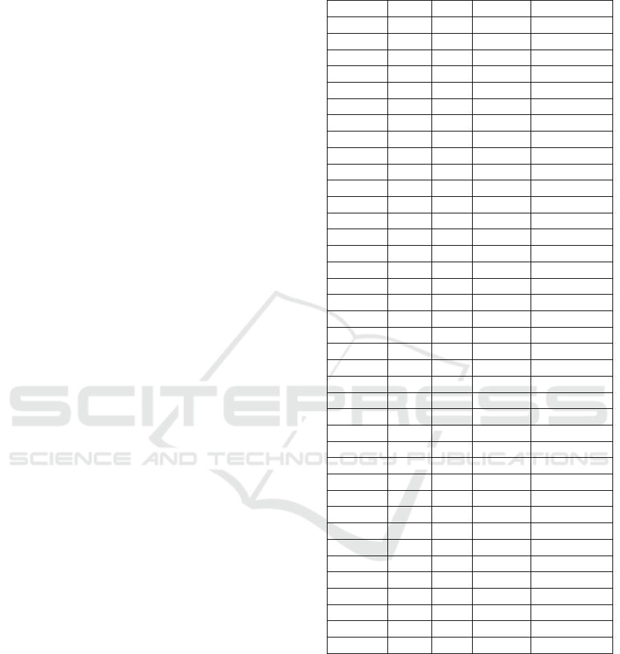
Table 1: Details of the considered data sets.
Syst. Vers. Inst. Nr. def. Percent def.
camel 1.0 339 13 3.83
camel 1.2 608 216 35.53
camel 1.4 872 145 16.63
camel 1.6 965 188 19.48
jedit 3.2 272 90 33.09
jedit 4.0 306 75 24.51
jedit 4.1 312 79 25.32
jedit 4.2 367 48 13.08
jedit 4.3 492 11 2.24
forest 0.6 6 1 16.67
forest 0.7 29 5 19.24
forest 0.8 32 2 6.25
ivy 1.1 111 63 56.76
ivy 1.4 241 16 6.64
ivy 2.0 352 40 11.36
log4j 1.0 135 34 25.19
log4j 1.1 109 37 33.95
log4j 1.2 205 189 92.20
lucene 2.0 195 91 46.67
lucene 2.2 247 144 58.30
lucene 2.4 340 230 67.65
poi 1.5 237 141 59.49
poi 2.0 314 37 11.78
poi 2.5 385 248 64.42
poi 3.0 442 281 63.58
synapse 1.0 157 16 10.19
synapse 1.1 222 60 27.08
synapse 1.2 256 86 33.59
velocity 1.4 196 147 75
velocity 1.5 214 142 66.36
velocity 1.6 229 78 34.06
xalan 2.4 723 110 15.21
xalan 2.5 803 387 48.19
xalan 2.6 885 411 46.44
xalan 2.7 909 898 98.79
xerces init 162 77 47.53
xerces 1.2 440 71 16.14
xerces 1.3 453 69 15.23
xerces 1.4 588 437 74.32
they can be read from Table 1, starting from 1 (as-
signed to the pair camel 1.0 - camel 1.2) and ending
with 28 (assigned to the pair xerces 1.3 - xerces 1.4).
Each component e
k
i
of each considered system, in
version k, is represented by a feature vector of 20
well-known object-oriented software metrics whose
complete description can be found in (Jureczko and
Madeyski, 2010). Therefore, e
k
i
= (e
k
i1
,e
k
i2
,. . . , e
k
i20
),
where e
k
i j
expresses the value of the jth software met-
ric computed for the software component e
k
i
. Each in-
stance has a numerical class label as well, denoting its
ENASE 2025 - 20th International Conference on Evaluation of Novel Approaches to Software Engineering
308

number of defects. As a pre-processing step, we have
transformed the number of defects into 0 for non-
defective and 1 for defective instances (having one or
more defects). This is in line with the vast majority of
the existing SDP approaches. As a consequence, SDP
can be formulated as a binary classification problem
approachable through supervised learning, the target
function to be learned being the mapping that assigns
to each software entity e
k
i
a class t(e
k
i
) ∈ {0, 1}.
In addition to the input features and the class label,
each component is identified in its version by a fully
qualified class name. This will be used to identify the
common instances between two versions (more de-
tails are presented in Section 3.3).
Since all the necessary information is available,
we can define the sets introduced in Section 3.1 for
all the pairs of consecutive versions derived from the
experimental data described in Table 1.
3.3 RQ1: Prevalence of Identical and
Very Similar Instances
In order to analyze the prevalence of closely related
instances, we study the data sets presented in Section
3.2. For every software system S, we consider every
pair of consecutive versions, denoted by S
v1
, S
v2
, and
compute for them five sets that have been defined
in Section 3.1: S
v1→v2
common, S
v1→v2
stayedDe f ,
S
v1→v2
stayedNonDe f , S
v1→v2
becameDe f and
S
v1→v2
becameNonDe f .
First, we compute how many elements of S
v2
ap-
pear in S
v1→v2
common, to see how many common
classes are in two consecutive versions. This infor-
mation could confirm whether there really are many
classes with the same name in two consecutive ver-
sions of a software system.
In order to determine whether an instance of S
v2
appears in S
v1
, we compare their name attribute values
which are the fully qualified names of the classes. Al-
though this simple approach might lead to false neg-
atives, since it is possible that a class was renamed
or moved to a different package from one version to
the next, the number of impacted classes is not sig-
nificant. The only exception is the ivy software sys-
tem, where the entire package structure changed after
version 1.4 (the package names changed completely
and the number of packages doubled). Consequently,
for the ivy system, we consider the unqualified (short)
class names of the instances for comparison.
Next, we analyze the distribution of the el-
ements from S
v1→v2
common in its four sub-
sets: S
v1→v2
stayedDe f , S
v1→v2
stayedNonDe f ,
S
v1→v2
becameDe f and S
v1→v2
becameNonDe f . We
consider this important since, as presented in Section
1, we believe that a good CVDP approach should be
able to identify the instances with changed labels and
the analysis will show whether there are many such
instances in our case studies.
The fact that the same class name appears in two
consecutive versions in itself is not a problem, since
class names are not used as an input feature for the
SDP models. However, if their feature vector is the
same, or highly similar, there might be a problem. In
order to investigate this, we first count how many el-
ements of S
v1→v2
common have exactly the same fea-
ture vector in both versions. After this, we look at the
distances between feature vectors in two ways:
1. We compute the distance between the feature vec-
tors in the two consecutive versions for the in-
stances from S
v1→v2
common, to see how close
they are to each other.
2. For every instance from S
v1→v2
common, we find
its nearest neighbor from S
v1
and check if the
nearest neighbor found has the same name.
This information is relevant, given that many ma-
chine learning models are based on the precondition
that similar instances should have the same label.
We opted to compute the Cosine distance between
the feature vectors, due to its scale-invariance. As-
suming that the two feature vectors are v
1
and v
2
, each
having ℓ features, denoted by v
11
,v
12
,..., v
1ℓ
respec-
tively v
21
,v
22
,..., v
2ℓ
the definition of the Cosine dis-
tance is given in Equation 9.
cos(v
1
,v
2
) = 1 −
∑
ℓ
i=1
v
1i
∗ v
2i
q
∑
ℓ
i=1
v
2
1i
∗
q
∑
ℓ
i=1
v
2
2i
(9)
3.4 RQ2: Influence of Identical and
Similar Train-Test Instances on the
Performance of CVDP Models
In order to answer RQ2, we analyze how the presence
of identical and similar train-test instances influences
the measures evaluating the performance of CVDP
models. For this, we train three different ML mod-
els in a CVDP scenario in which we use as training
data an entire version v1 of a software system, while
considering the following testing sets:
1. The training data, v1 - this is not a recommended
evaluation scenario, but we use the training data
for testing too in order to see how well the model
learned the training data.
2. All instances of the next version, v2 - this is the
prevalent CVDP evaluation scenario, considered
in a large proportion of papers from the literature.
Cross-Version Defect Prediction: Does Excessive Train-Test Similarity Affect the Reliability of Evaluation?
309

3. All instances from S
v1→v2
changedLabel - these
are the common instances for which the label
changed from one version to the next. As already
stated in Section 1, it is crucial that a good CVDP
model classifies these instances correctly.
4. All instance from S
v1→v2
sameLabel - to compare
the results with those for the changed labels.
5. All instances from S
v1→v2
new - these are the in-
stances newly introduced in version v2.
We have opted to run the above-mentioned train-
test scenarios considering three different ensemble
learning models: Random Forest (RF), AdaBoost
and Gradient Boosting (XGBoost), motivated by their
suitability for imbalanced problems (Zhao et al.,
2022a) like SDP (and, as can be seen in Table 1, the
experimental SDP data sets are indeed imbalanced).
The analyses for both research questions were im-
plemented in Python, using scikit-learn (Pedregosa
et al., 2011). An important parameter for all three
methods is the number of trees to be considered. For
our experiments, we used the minimum value be-
tween 100 (which is the default value for RF and XG-
Boost) and a quarter of the training instances. For the
other hyperparameters, the default values were used.
Since all these algorithms imply randomness, we have
run the experiments 30 times and will report average
values for these runs.
Since SDP is framed as a binary classification
problem, the performance is measured based on the
four values from the confusion matrix. There are
many different performance measures used in the lit-
erature, but, due to lack of space, we select two of
them: AUC and MCC. Both are recognized as par-
ticularly good evaluation measures in case of imbal-
anced data (Zhao et al., 2022a). MCC has the ad-
vantage of considering all 4 values in the confusion
matrix. For both measures, higher values mean better
performance. AUC has values between 0 and 1, where
randomly guessing the label would mean an AUC of
0.5. MCC, being a correlation coefficient, takes val-
ues between -1 and 1, a value of 0 meaning that there
is no correlation between the predicted and the actual
labels.
4 RESULTS AND ANALYSIS
In this section we will present and interpret the results
of the analyses described in Sections 3.3 and 3.4.
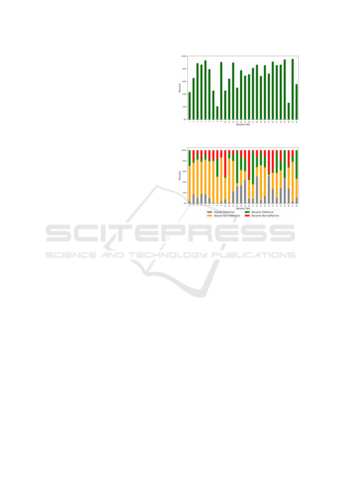
Figure 1: Percent of common files in the considered data
sets.
Figure 2: Percent of changed and unchanged labels in the
considered data sets for the common instances.
4.1 RQ1: Prevalence of Identical and
Similar Instances
For every pair of consecutive versions, v1 and v2,
from those presented in Section 3.2, Figure 1 depicts
the percentage of instances from v2 which appear in
v1. We can see that these percentages are quite high,
there being only two pairs (forest 0.6 - forest 0.7 and
xerces init - xerces 1.2) where the value is below 40%.
For 13 pairs, the percentages are above 80%. The av-
erage value is 72%, while the median is 79%. These
significant percentages confirm our intuition that, in
most cases, two consecutive versions of a software
system share a lot of common classes.
Figure 2 presents how these common classes (ele-
ments of the set S
v1→v2
common) are divided into the
four possible subsets, depending on their labels. The
gray and orange bars represent the instances for which
the labels did not change, while the red and green ones
represent the instances for which the labels changed.
We can see that in general, most of the instances keep
the same label (the mean is 65% and the median is
67%). However, there are a few pairs, where more
classes changed their labels, 6 of them have values
greater than or equal to 50%, the maximum being
64% for the poi 2.0 - poi 2.5 pair, closely followed by
ENASE 2025 - 20th International Conference on Evaluation of Novel Approaches to Software Engineering
310

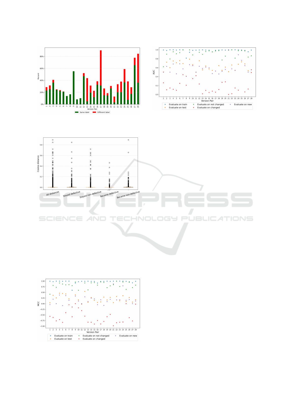
Figure 3: Percentage of identical instances and their divi-
sion into same-label and different-label categories in the
common instances of the considered data set.
Figure 4: Cosine distance between common instances.
the log4j 1.1 - log4j 1.2 pair with 62%. As we have
already mentioned, these instances with changed la-
bels are the ones which should be identified by a good
CVDP approach.
While Figures 1 and 2 considered the classes with
the same name (called common instances), on Fig-
ure 3 we can see the percentage of the common in-
stances which have identical feature vectors. We can
see that there are big differences in the values for dif-
ferent pairs, the mean value being 35% with a median
of 31%. There are 3 pairs with a value around 80%:
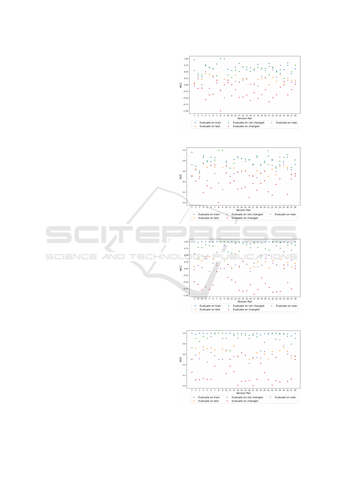
Figure 5: MCC values for the Random Forest models, for
the considered data sets.
Figure 6: AUC values for the Random Forest models, for
the considered data sets.
poi 2.0 - poi 2.5, xerces 1.2 - xerces 1.3 and xerces
1.3 - xerces 1.4. On the other side, we have values
around 10% for the two pairs considered for the ivy
data set. What is particularly interesting on Figure 3
is the height of the red bars. They represent instances
for which the feature vectors are identical, but the la-
bel changed. This situation can appear if the source
code did change, but the considered features are not
sensitive enough to detect the source code changes,
or they can be due to labeling error. In order to deter-
mine the exact situation, a more detailed analysis on
the exact source code is needed, but this is outside the
scope of this paper.
While the red bars in Figure 3 represent instances
that will very likely be classified incorrectly, the green
bars represent those instances that are exactly the
same in both versions, which means that they repre-
sent an overlap between the train and the test set of
the ML-based CVDP models.
Next, for the common instances, we have com-
puted the cosine distance between their feature vec-
tors in the two versions. Figure 4 plots these dis-
tances, aggregated over all version pairs, but di-
vided into categories based on whether the labels
changed (and how) or not between them. We can
see that the median of these values is actually very
close to 0. More specifically, it is 0.0004 for in-
stances which stayed defective, 2.220E-16 for in-
stances which stayed non-defective, 2.22E-16 for in-
stances which became defective and 0.0002 for in-
stances which became non-defective. While there are
obviously outliers and there are pairs with distance as
big as 0.89, there are only 101 classes out of the total
8608 with a distance greater than 0.1. This shows that
most common classes are not changed a lot (or the
change is not reflected by the software metrics used
as features). Also, it does not seem to be a pattern in
the values depending on the label change.
We have looked at the average cosine distance for
each version pair, considering the same 5 categories
Cross-Version Defect Prediction: Does Excessive Train-Test Similarity Affect the Reliability of Evaluation?
311

as in case of Figure 4. The exact figure is omitted due
to lack of space. As expected, the average values are
very low, even the maximum is below 0.06. Similarly
to Figure 4, there does not seem to be a pattern in
the distances for different changes in the label. For
11 version pairs the maximum average distance is for
instances which stayed defective, for 2 pairs it is for
instances which stayed non-defective, for 5 pairs it
is for instances which became defective and for the
remaining 10 pairs it is for instances which became
non-defective.
Finally, we have counted how many of the com-
mon instances have as nearest neighbor in v1 the in-
stance with the same name. The median value for the
28 version pairs is 73%, with a minimum of 36% (for
the pair ivy 1.1 - ivy 1.4) and a maximum is 1 (the pair
forrest 0.6 - forrest 0.7).
In conclusion, we can answer RQ1 saying that on
average, 72% of the classes from a version of a soft-
ware system are in common with the previous version
and on average 35% of them are actually identical, al-
though they might have different labels. So when a
ML model is trained on a version and tested on the
next one, there will be instances in the test set which
were part of the train set as well. Moreover, the in-
stances which are not identical have, on average, a
very small cosine distance between their feature vec-
tor in the two versions.
4.2 RQ2: Influence of Identical and
Similar Instances
The results of the experiments presented in Section
3.4 can be visualized on Figures 5, 6 (for the RF mod-
els), 7, 8 (for the AdaBoost models) and 9, 10 (for the
XGBoost models). We can observe that the patterns
seem to be the same for both MCC and AUC, so in
the following, due to lack of space, we will detail the
results based on the MCC values.
In all figures we can observe that the evaluation
on the train data (the blue asterisks) produces very
good results: with the exception of the forest 0.6 -
forest 0.7 pair having an MCC of 0.6, the MCC is
above 0.9 for RF. XGBoost also leads to MCC values
above 0.9 (with the exception of the two pairs from
forest) while AdaBoost has a slightly worse perfor-
mance, with MCC around 0.6-0.7 for most version
pairs (but with a minimum of 0.31). RF and XG-
Boost seem to have managed to learn the train data
very well.
If we are looking at the orange asterisks, repre-
senting the use of the next version for testing, we can
see that the performance is not as good as on the train-
ing data, but in most cases, still acceptable: MCC is
Figure 7: MCC values for the AdaBoost models for the con-
sidered data sets.
Figure 8: AUC values for the AdaBoost models for the con-
sidered data sets.
Figure 9: MCC values for the XGBoost models, for the con-
sidered data sets.
Figure 10: AUC values for the XGBoost models, for the
considered data sets.
ENASE 2025 - 20th International Conference on Evaluation of Novel Approaches to Software Engineering
312

between -0.157 and 0.54 for RF, between -0.23 and
0.43 for AdaBoost and between 0 and 0.55 for XG-
Boost. The purple asterisks, representing the evalu-
ation on the new instances, are pretty much overlap-
ping with the orange ones, suggesting that the mod-
els had moderate performance in classifying new in-
stances.
When considering the common instances for
which the class labels did not change in the two ver-
sions (denoted by green asterisks), we can see the
same excellent performance as seen in case of eval-
uating on the train data. This is most probably due
to the fact that those exact instances were seen during
the training phase of the models.
Finally, the performance on those instances that
changed their label is indicated by the red asterisks.
Correctly identifying them is extremely important.
Yet, the MCC values for them are mostly negative,
suggesting that there is a negative correlation between
the predicted values and the actual ones: for RF there
are only 2 MCC values of 0, the rest being negative,
while the minimum value is -0.98. AdaBoost, since it
did not learn the train data that well, has a few positive
MCC values for the instances with changed labels, but
the maximum is still only 0.17. Finally, XGBoost has
MCC values between -0.95 and 0.
Furthermore, we have computed the Pearson cor-
relations between the two performance measures of
the three models tested on the entire test version v2
(which is the standard CVDP scenario) and the per-
centage of instances in different subsets of v2. The
results are depicted in Figure 11. We can see that
there is a positive correlation of around 0.5 between
the performance values and the percentage of com-
mon instances (dark blue bars), meaning that the more
common instances we have between v1 and v2, the
higher the performance measures. There is an even
stronger correlation between the performance values
and the percentage of common instances with iden-
tical labels (light blue bars). Somehow surprisingly,
the percentage of identical instances in the common
ones (orange bars) and the percentage of identical in-
stances with the same label (green bars) is less cor-
related with the performance than the previous two
categories. Finally, as expected, the percentage of
common instances with different labels (purple bars)
is negatively correlated with the performance, the cor-
relation value being around -0.5. This points out that
the more common instances with changed labels, the
worst the performance measure.
Another interesting observation is that the corre-
lations for AdaBoost are in general lower than those
of RF and XGBoost. This might be related to the fact
that AdaBoost was the model where the performance
measures on the train data and on the common in-
stances with the same label were lower than for the
other two models. AdaBoost did not learn the train
data so well, so it is less influenced by the occurrence
of common instances.
From the above analysis, we can answer RQ2 by
saying that the presence of identical and similar in-
stances in two consecutive versions strongly influ-
ences the performance of CVDP approaches. Com-
puting the performance for the entire version will hide
the fact that the model performs poorly on the impor-
tant instances whose labels changed from one version
to another. The evaluation of the new instances does
not seem to be influenced by this issue, as on them
the classification performance is in line with that com-
puted for the entire version v2.
5 THREATS TO VALIDITY
Internal validity. For our experiments, one internal
validity aspect is the randomness in the considered
ML algorithms. In order to mitigate this, we have
repeated the experiments 30 times and considered av-
erage values for the performance measures.
External validity. A common external validity is-
sue for applying ML models for software engineer-
ing problems is that the results might not generalize
for other ML models and/or other data sets. We tried
to mitigate this by considering all data sets from the
seacraft repository that fit our requirements. These
are also the data sets that appear most frequently in
the related literature thus the presented insights affect
a large proportion of the literature. Nevertheless, in
the future we will repeat the experiments for other
data sets with different feature spaces, for ex. seman-
tic, syntactic or code change metrics.
Construct validity. In our case, construct valid-
ity refers to the selection of performance measures
and baseline algorithms. We have considered two
performance measures which are suitable and often
used for imbalanced data sets (such as SDP data sets):
AUC and MCC. Both show the same conclusions. For
comparison, we have used only three relatively sim-
ple baseline methods, but our goal was not to assess
their predictive performance, but to show how that
performance changes for different parts of the test
data. Another aspect of the validity of the construct
is the reliance on the labels and the metric values
of the considered data sets. As presented in Section
4.1, there are identical instances with changed labels,
which could be the result of labeling errors. Since
these data sets are used a lot for SDP (not just cross-
version, but also cross-project and within-version),
Cross-Version Defect Prediction: Does Excessive Train-Test Similarity Affect the Reliability of Evaluation?
313

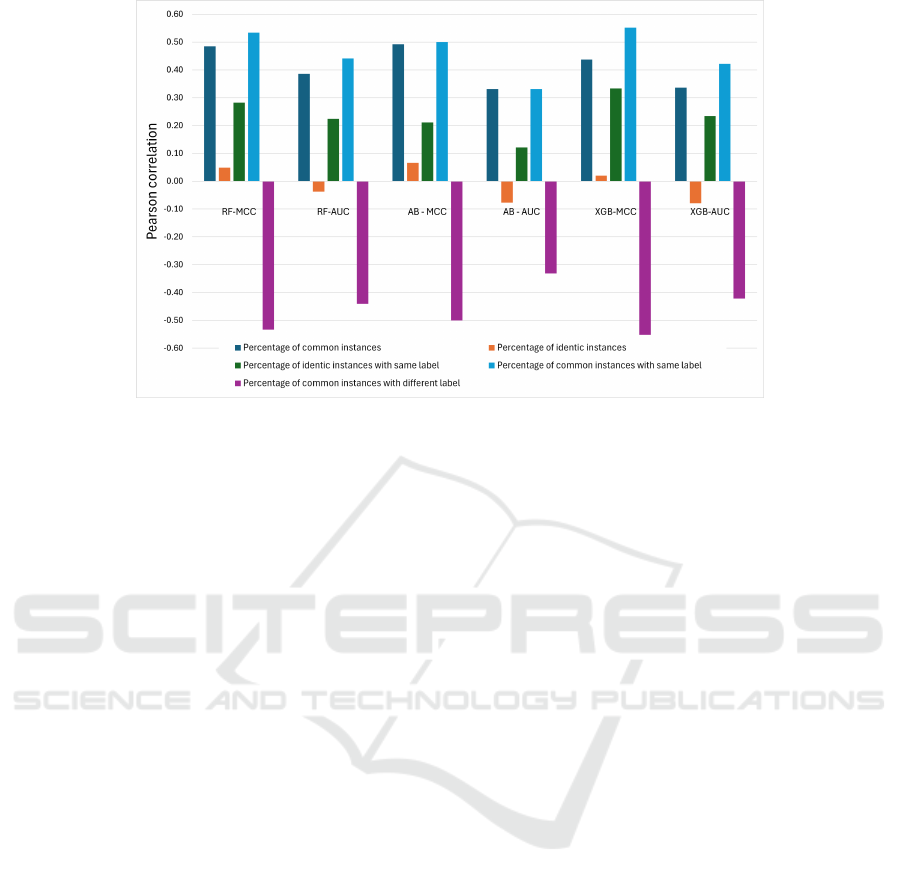
Figure 11: Pearson correlations between performance measures and percentage of common and identical instances. RF stands
for Random Forest, AB for AdaBoosting and XGB stands for XGBoost.
we consider them trustworthy. In addition, the con-
clusions of our study apply to all data sets considered,
not just those with a high number of such instances.
6 CONCLUSIONS
In this paper we have shown, through an empirical
study, that the performance of CVDP approaches is
influenced by train-test similarity. By analyzing 28
software version pairs, we have confirmed that identi-
cal and highly similar instances are frequent in suc-
cessive software versions. By employing three en-
semble learners, we have also shown that using the
standard ”train the model on version v1 and evalu-
ate it on the next version v2” CVDP scenario leads
to overly optimistic performance indicators due to
these instances, which hides the extremely poor per-
formance of the models in predicting the labels that
changed from v1 to v2. We seek to raise awareness to
this issue and to work towards a better evaluation of
CVDP approaches.
There are many directions in which we envision
continuing this research. First, it would be worth
investigating whether the presence of identical in-
stances with different labels is the result of labeling
errors or are due to not sufficiently sensitive soft-
ware features. Besides this, we aim to replicate the
study using different software representations based
on semantic features automatically extracted from the
source code or code change metrics, or embeddings, a
really popular code representation nowadays. Extend-
ing the investigation by employing additional classi-
fiers is another future direction taken into consider-
ation. Finally, we consider exploring how the eval-
uation of CVDP models could be improved, while
giving enough attention to the performance on the
instances whose labels changed. We will analyze
why models fail on instances with changed labels and
study how to build models with better generalization
capabilities.
ACKNOWLEDGEMENTS
The publication of this article was supported by the
2024 Development Fund of the UBB.
REFERENCES
(2017). The SEACRAFT repository of empirical software
engineering data.
Amasaki, S. (2017). On applicability of cross-project de-
fect prediction method for multi-versions projects. In
Proceedings of the 13th International Conference on
Predictive Models and Data Analytics in Software En-
gineering, page 93–96. ACM.
Amasaki, S. (2018). Cross-version defect prediction using
cross-project defect prediction approaches: Does it
work? In Proceedings of the 14th International Con-
ference on Predictive Models and Data Analytics in
Software Engineering, page 32–41. ACM.
Amasaki, S. (2020). Cross-version defect prediction: use
historical data, cross-project data, or both? Empirical
Software Engineering, 25:1573 – 1595.
Bennin, K. E., Toda, K., Kamei, Y., Keung, J., Monden,
A., and Ubayashi, N. (2016). Empirical evaluation
of cross-release effort-aware defect prediction models.
ENASE 2025 - 20th International Conference on Evaluation of Novel Approaches to Software Engineering
314

In 2016 IEEE International Conference on Software
Quality, Reliability and Security, pages 214–221.
Chen, M. and Ma, Y. (2015). An empirical study on predict-
ing defect numbers. In International Conference on
Software Engineering and Knowledge Engineering.
Chen, X., Zhang, D., Zhao, Y., Cui, Z., and Ni, C. (2019).
Software defect number prediction: Unsupervised vs
supervised methods. Information and Software Tech-
nology, 106:161–181.
Cohen, M., Rokach, L., and Puzis, R. (2022). Cross version
defect prediction with class dependency embeddings.
ArXiv, abs/2212.14404.
Fan, G., Diao, X., Yu, H., Yang, K., Chen, L., and Vitiello,
A. (2019). Software defect prediction via attention-
based recurrent neural network. Sci. Program., 2019.
Harman, M., Islam, S., Jia, Y., Minku, L. L., Sarro, F., and
Srivisut, K. (2014). Less is more: Temporal fault pre-
dictive performance over multiple hadoop releases. In
Le Goues, C. and Yoo, S., editors, Search-Based Soft-
ware Engineering, pages 240–246. Springer.
Huo, X. and Li, M. (2019). On cost-effective software de-
fect prediction: Classification or ranking? Neurocom-
puting, 363:339–350.
Jureczko, M. and Madeyski, L. (2010). Towards identify-
ing software project clusters with regard to defect pre-
diction. In Proceedings of the 6th international con-
ference on predictive models in software engineering,
pages 1–10.
Kabir, M. A., Keung, J., Turhan, B., and Bennin, K. E.
(2021). Inter-release defect prediction with feature se-
lection using temporal chunk-based learning: An em-
pirical study. Appl. Soft Comput., 113(PA).
Kabir, M. A., Keung, J. W., Bennin, K. E., and Zhang, M.
(2020). A drift propensity detection technique to im-
prove the performance for cross-version software de-
fect prediction. In 2020 IEEE 44th Annual Computers,
Software, and Applications Conference (COMPSAC),
pages 882–891.
Kabir, M. A., Rehman, A. U., Islam, M. M. M., Ali, N., and
Baptista, M. L. (2023). Cross-version software defect
prediction considering concept drift and chronological
splitting. Symmetry, 15(10).
Li, Y., Su, J., and Yang, X. (2018). Multi-objective vs.
single-objective approaches for software defect pre-
diction. In Proceedings of the 2nd International Con-
ference on Management Engineering, Software Engi-
neering and Service Sciences, page 122–127. ACM.
Lu, H., Kocaguneli, E., and Cukic, B. (2014). Defect pre-
diction between software versions with active learn-
ing and dimensionality reduction. 2014 IEEE 25th
International Symposium on Software Reliability En-
gineering, pages 312–322.
Ouellet, A. and Badri, M. (2023). Combining object-
oriented metrics and centrality measures to predict
faults in object-oriented software: An empirical val-
idation. Journal of Software: Evolution and Process.
Pedregosa, F., Varoquaux, G., Gramfort, A., Michel, V.,
Thirion, B., Grisel, O., Blondel, M., Prettenhofer,
P., Weiss, R., Dubourg, V., Vanderplas, J., Passos,
A., Cournapeau, D., Brucher, M., Perrot, M., and
Duchesnay, E. (2011). Scikit-learn: Machine learning
in Python. Journal of Machine Learning Research,
12:2825–2830.
Shukla, S., Radhakrishnan, T., Kasinathan, M., and Neti,
L. B. M. (2016). Multi-objective cross-version defect
prediction. Soft Computing, 22:1959 – 1980.
Sun, B. (2024). Bert-based cross-project and cross-version
software defect prediction. Applied and Computa-
tional Engineering, 73:33–41.
Wang, S., Liu, T., and Tan, L. (2016). Automatically learn-
ing semantic features for defect prediction. In Pro-
ceedings of the 38th International Conference on Soft-
ware Engineering, page 297–308. ACM.
Wang, Z., Tong, W., Li, P., Ye, G., Chen, H., Gong, X.,
and Tang, Z. (2022). BugPre: an intelligent software
version-to-version bug prediction system using graph
convolutional neural networks. Complex & Intelligent
Systems, 9.
Xu, Z., Li, S., Luo, X., Liu, J., Zhang, T., Tang, Y., Xu, J.,
Yuan, P., and Keung, J. (2019). TSTSS: A two-stage
training subset selection framework for cross version
defect prediction. J. Syst. Softw., 154(C):59–78.
Xu, Z., Li, S., Tang, Y., Luo, X., Zhang, T., Liu, J., and
Xu, J. (2018a). Cross version defect prediction with
representative data via sparse subset selection. In Pro-
ceedings of the 26th Conference on Program Compre-
hension, page 132–143. ACM.
Xu, Z., Liu, J., Luo, X., and Zhang, T. (2018b). Cross-
version defect prediction via hybrid active learning
with kernel principal component analysis. In IEEE
25th International Conference on Software Analysis,
Evolution and Reengineering, pages 209–220.
Yang, X. and Wen, W. (2018). Ridge and lasso regres-
sion models for cross-version defect prediction. IEEE
Transactions on Reliability, 67:885–896.
Yu, X., Rao, J., Liu, L., Lin, G., Hu, W., Keung, J. W.,
Zhou, J., and Xiang, J. (2024). Improving effort-
aware defect prediction by directly learning to rank
software modules. Information and Software Technol-
ogy, 165:107250.
Zhang, J., Wu, J., Chen, C., Zheng, Z., and Lyu, M. R.
(2020). CDS: A cross–version software defect pre-
diction model with data selection. IEEE Access,
8:110059–110072.
Zhang, N., Ying, S., Ding, W., Zhu, K., and Zhu, D. (2021).
WGNCS: A robust hybrid cross-version defect model
via multi-objective optimization and deep enhanced
feature representation. Inf. Sci., 570(C):545–576.
Zhao, Y., Wang, Y., Zhang, D., and Gong, Y. (2022a). Elim-
inating the high false-positive rate in defect prediction
through bayesnet with adjustable weight. Expert Sys-
tems, 39.
Zhao, Y., Wang, Y., Zhang, Y., Zhang, D., Gong, Y., and Jin,
D. (2022b). ST-TLF: Cross-version defect prediction
framework based transfer learning. Information and
Software Technology, 149:106939.
Cross-Version Defect Prediction: Does Excessive Train-Test Similarity Affect the Reliability of Evaluation?
315